Black Hole - Bulge Relationship of Post-Starburst Quasars at $z\sim 0.3$

Abstract

The M${}_{\rm BH}-\sigma_{*}$ relation has been studied extensively for local galaxies, but to date there have been scarce few direct measurements of stellar velocity dispersions for systems beyond the local universe. We investigate black hole and host galaxy properties of six “post-starburst quasars” at $z\sim 0.3$. Spectra of these objects simultaneously display features from the active nucleus including broad emission lines and a host galaxy Balmer absorption series indicative of the post-starburst stellar population. These are the first measurements of $\sigma_{*}$ in such objects, and we significantly increase the number of directly-measured non-local objects on the M${}_{\rm BH}-\sigma_{*}$ diagram. The “post-starburst quasars” of our sample fall on or above the locally defined M${}_{\rm BH}-\sigma_{*}$ relation, a result that is consistent with previous M${}_{\rm BH}-\sigma_{*}$ studies of samples at $z>0.1$. However, they are generally consistent with the M${}_{\rm BH}-$L_bulge relation. Futhermore, their location on the Faber-Jackson relation suggests that some of the bulges may be dynamically peculiar.

1. Introduction

The M${}_{\rm BH}-\sigma_{*}$ relation (Ferrarese & Merritt, 2000; Gebhardt et al., 2000; Gültekin et al., 2009; Woo et al., 2010) has been extensively studied in both active and inactive galaxies at low redshifts. The existence of this and other black hole - host galaxy scaling relations (Magorrian et al., 1998; McLure & Dunlop, 2002) implies that the growth of black holes is intimately connected with that of the host galaxies. However, the mechanism by which this growth is regulated is still an open matter.

One proposed mechanism is through black hole accretion feedback. Di Matteo et al. (2005) show that only a modest amount of the accretion energy is required to shut down star formation in the host galaxy. Their simulations of galaxy mergers reproduce the local M${}_{\rm BH}-\sigma_{*}$ relation with only $\sim 5$% of the AGN luminosity being thermodynamically coupled to the surrounding gas. On the other hand, the need for accretion feedback is not clear. Peng (2007) argues that mergers between galaxies (major and minor) naturally leads to a tight log-linear M_BH-M_bulge relation. To investigate the co-evolution of black holes with their hosts, it is necessary to measure the relation at higher redshifts.

Robertson et al. (2006) study the theoretical evolution in the M${}_{\rm BH}-\sigma_{*}$ relation by simulating galactic mergers and including both supernova and black hole feedback. They predict that the slope of the relation remains roughly constant out to redshift $z=6$, while the scaling of the relation slightly decreases due to an evolving Faber-Jackson relation. The effect of this would be that $\sigma_{*}$ increases for a given M_BH as a function of redshift. Conversely, Croton (2006) predicts that the M_BH-M_bulge relation evolves in the opposite sense, i.e., black hole mass increases with redshift for a given bulge mass.

Observational investigations into the evolution of the M${}_{\rm BH}-\sigma_{*}$ relation face difficulties. The sphere of influence of the black hole cannot be resolved at high redshifts, thus the methods using stellar or gas dynamics (Kormendy & Richstone, 1995) to measure M_BH in the local universe are unavailable. Alternatively, one can use the virial method to estimate black hole masses, which invokes AGN broad line widths and the R_BLR-L₅₁₀₀ relation (Kaspi et al., 2000; Bentz et al., 2009a). However, in type-1 active galactic nuclei (AGN), the active nucleus often outshines the host, drowning out stellar features in the spectra. Despite this effect, Woo et al. (2006, 2008) studied a sample of Seyfert galaxies and found that black holes at $z=0.36$ and $z=0.57$ were over-massive for their given stellar velocity dispersions compared to the local relation. Canalizo et al. (2012) avoid the problem of an over-powering AGN continuum by studying dust-reddened quasars between $0.14<z<0.37$, which have spectra that show both active nucleus and host galaxy features. They find a result similar to Woo et al. in that reddened quasars fall above the local M${}_{\rm BH}-\sigma_{*}$ relation. The red quasars of Canalizo et al. also fall above the M${}_{\rm BH}-$L_bulge relation, supporting the notion that the black holes are over-massive compared to their bulges.

Other recent studies have discussed regimes in which the local inactive galaxy relation may not hold. Graham et al. (2011) calibrate the M${}_{\rm BH}-\sigma_{*}$ relation using elliptical, barred and unbarred galaxies and find that the slope of the M${}_{\rm BH}-\sigma_{*}$ relation can vary according to morphology. Conversely, Beifiori et al. (2011) and Vika et al. (2011) find no correlation between black hole mass and Sérsic index, n. At the low-mass end of the M${}_{\rm BH}-\sigma_{*}$ relation, Xiao et al. (2011) find little difference in the relation as defined by barred and unbarred Seyfert 1 galaxies. Xiao et al. also state that inclination angle of a galactic disk components may increase the scatter of the M${}_{\rm BH}-\sigma_{*}$ relation. This is consistent with the results of Bennert et al. (2011), who find that $\sigma_{*}$ can be biased to larger or smaller values by the disk component of the galaxy. Recently, McConnell et al. (2011a, b) showed that brightest cluster galaxies have black holes that are significantly more massive than predicted from the M${}_{\rm BH}-\sigma_{*}$ relation given their velocity dispersions.

In this paper we exhibit the first results of our investigation of the M${}_{\rm BH}-\sigma_{*}$ relation using a sample of AGN whose host galaxies contain luminous post-starburst stellar populations between redshifts $0.2<z<0.4$. Brotherton et al. (2012, (in preparation)) catalog a subset of quasars with strong Balmer absorption series visible in their spectra. These “post-starburst quasars” (PSQs) are a convenient case for the study of the M${}_{\rm BH}-\sigma_{*}$ relation at higher$-z$, because spectra of these objects simultaneously show the broad emission lines distinctive of an active black hole as well as strong stellar absorption lines indicative of a post-starburst stellar population in the host galaxies. The moniker “post-starburst quasars” is not a definitive classification of the objects’ luminosities. While some are luminous enough to be considered quasars, others are not. To be consistent with previous work (Cales et al., 2011; Brotherton et al., 2010), we will continue to refer to the sample as “post-starburst quasars”.

In this paper we present the stellar velocity dispersions ($\sigma_{*}$) and black hole masses (M_BH) of six post-starburst quasars as measured from spectroscopy performed with the Low Resolution Imaging Spectrograph (LRIS) on Keck I. Each of these PSQs were observed with $HST$ ACS F606W as part of a snapshot program (10588, PI Brotherton, M.). These images and a detailed morphological study of the host galaxies are presented in Cales et al. (2011). In our analysis we rely on photometry reported by Cales et al., and we adopt the same cosmology that they use: a flat universe with H${}_{\rm o}=73$ km s^-1, $\Omega_{\rm M}=0.27$, and $\Omega_{\Lambda}=0.73$. The paper is organized as follows: we discuss the sample and observations in section 2, describe our spectral fitting code and $\sigma_{*}$ measurements in section 3, and discuss virial black hole mass calculations in section 4. We present our main results and discussion of possible biases in sections 5 and 6, respectively.

2. Sample and Observations

We present results for six post-starburst quasars from an overall sample of 609 PSQs selected from the Sloan Digital Sky Survey (SDSS) DR3 (Abazajian et al., 2005) that show both strong Balmer series absorptions and broad emission lines. The full details of the sample selection are described in Brotherton et al. (2012, (in preparation)), but see also Cales et al. (2011) and Brotherton et al. (2010). Briefly: objects in the sample have total Balmer equivalent widths H${}_{total}=$ EW_Hδ $+$ EW_H8 $+$ EW_H9 $>2$ Å. H$\epsilon$ was excluded from this measurement, because it can be blended with Ca II. The Balmer break flux ratio was defined by two 100 Å regions starting at restframe wavelengths 3740 and 3985 Å, and the selection criterion was set at $f_{3985\rm\AA}/f_{3740\rm\AA}>0.9$. The continuum S/N in the SDSS spectra were $>8$ as measured between 4150 and 4250 Å.

We observed six post-starburst quasars of the sample using the Low Resolution Imaging Spectrometer (Oke et al., 1995; Rockosi et al., 2010) at Keck I in September 2010. Conditions were excellent with $\sim 0\farcs 6$ seeing. We employed both the red and blue side cameras of LRIS to obtain broad spectral coverage. With this coverage we are able to observe the Balmer series (except for H$\alpha$ and H$\beta$) of our science targets. We observed several individual stars to construct host galaxy templates on nights in May 2010 and September 2010 using the same instrumental setup as for our science targets.

We observed all of the sample targets with the same setup with LRIS blue and red sides. On the blue side we used the 600/4000 grism, and on the red side we used the 1200/7500 grating. This setup covers observed frame 3100 Å to 6250 Å. Because of the small dispersion in redshift of our science targets, this resulted in slightly different rest-frame wavelength coverage. With this setup we observed the quasar continuum and Mg II emission line on the blue side and the Balmer series on the red side. For one object, SDSS $0237-0101$, we also observed a second red region out to observed frame 7800 Å. For each target we placed a 1″ observing slit across the nucleus of the object and oriented it according to the parallactic angle. In Fig. 1, we show $HST$ ACS F606W images of our sample with the LRIS slit overplotted (proposal 10588; PI: Brotherton, M.). Table 1 shows the redshift, exposure times, SDSS $r$ mag, the aperture size used to extract the spectra, and the morphology of each science target.

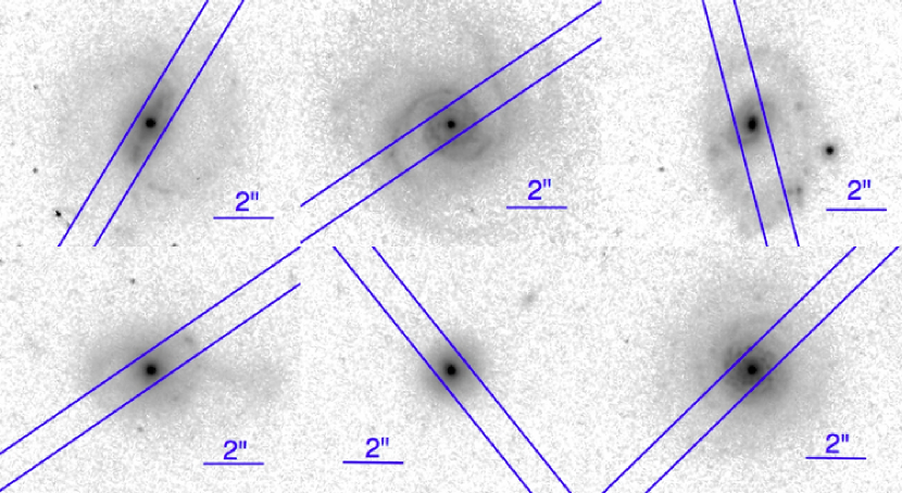
Figure 1.— HST ACS F606W images of our sample (Proposal ID 10588; PI: Brotherton, M.). North is up and East is to the left in each of the images. The LRIS slit was placed at parallactic angle with a 1$\arcsec$ width. Top: $0030-1035$, $0057+0100$, and $0237-0101$. Bottom: $2102+0005$, $2118+0056$, and $2306-0100$.

Table 1Observations

N	Object	redshift	exp time (s)	r [mag]	ap radius (″)	morphology
1	SDSS $003043.59-103517.6$	0.294	1200	18.41	2.52	bulge+disk, barred-spiral
2	SDSS $005739.19+010044.9$	0.253	1200	17.91	2.28	bulge+disk, spiral
3	SDSS $023700.31-010130.4$	0.344	2400	18.19	0.22	bulge+disk, spiral
4	SDSS $210200.42+000501.9$	0.329	2400	18.66	0.98	elliptical
5	SDSS $211838.12+005640.6$	0.384	1200	18.36	0.44	elliptical
6	SDSS $230614.18-010024.4$	0.267	1200	18.76	0.26	bulge+disk

We followed standard data reduction procedures using the NOAO package in IRAF. First we removed bias levels using the overscan region and cosmic rays from the 2D spectra using the L.A.Cosmic routine (van Dokkum, 2001), and corrected for flat fields. We derived a wavelength solution from Hg, Ne, Ar, Cd, and Zn arc lamps and shifted individual spectra taken throughout the night based on sky lines. We fit sky background with a low-order polynomial and subtracted the fit from the 2D spectra. Based on the measurements of Cales et al. (2011), we extracted each spectrum using an aperture width equal to twice the effective radius of the host’s bulge componet (i.e., center $\pm$R_eff). This is consistent with what has been done in previous studies (Gebhardt et al., 2000; Bennert et al., 2011) and avoids added uncertainty from aperture corrections when measuring stellar velocity dispersions. We used three standard stars observed throughout the night at parallactic angle to derive a flux calibration with data from Massey et al. (1988) and Massey & Gronwall (1990). We also corrected for Galactic reddening using the extinction values of Schlegel et al. (1998) calculated at sky positions by the NASA Extragalactic Database extinction calculator. We used the IRAF task deredden, which uses the extinction function of Cardelli et al. (1989) with the input extinction values to correct the spectra.

We recovered the spectral region from 3100 to 7250 Å with the 600 line mm^-1 grism and 1200 line mm^-1 grating blazed at 7500 Å for each template star. The S/N of the template stars spectra was $\geq$1000. Table 2 lists the stars and their spectral types used to create host galaxy templates in this project. We conducted the same data reduction procedures on the observed template stars as on the post-starburst quasars with the additional step of correcting for observed radial velocities.

Table 2Template Stars

Star	Sp Type
HD 93700	A0
HD 94980	A3
BD +182402	A5
HD 95002	F0
BD +182401	F5
HD 95958	F8
HD 97127	G0
HD 95676	G5
HD 184850	G8
HD 95437	K0
HD 230519	K2
HD 347822	K2
HD 347838	K5
HD 96761	K5
HD 347857	K7
BD +212255	M0
GSC $01562-00224$	M8

The blue and red sides of LRIS have different spectral resolutions. The Balmer series fell on the blue side of LRIS for the template stars, but was shifted to longer wavelengths for the quasars in the sample. Before combining our spectra and fitting, we convolved the red side of the quasar spectra with a Gaussian to match the resolution of the blue side. We achieved an intrinsic resolution of $\sigma$ = 90 km s^-1 for the lowest redshift object (SDSS $0030-1035$; $z$=0.253) at rest-frame 3839 Å. We achieved resolution of $\sigma$= 82 km s^-1 for the highest redshift object (SDSS $2118+0056$; $z$=0.384) at rest-frame 3475 Å.

3. Stellar Velocity Dispersion

3.1. Fitting Code

To measure the stellar velocity dispersion of each host galaxy, we follow a direct fitting method that has been used extensively in previous studies. Barth et al. (2003) use the direct fitting method to fit the spectra of BL Lac objects. More recently it was employed by Xiao et al. (2011) to fit a sample of Seyfert 1 host galaxies, and by Greene et al. (2010b) to fit the spectra of H₂O megamasers. Canalizo et al. (2012) use the method to fit the host galaxies of dust-reddened quasars.

We model the spectra with contributions from both the host galaxy and the active nucleus. The host template is constructed with a composite of stellar spectra taken with the same instrumental setup (see § 3.2 for details) and broadened with a Gaussian in order to simulate the stellar velocity dispersion of the host galaxy. We include a power-law continuum attributed to the intrinsic active nucleus spectrum. We also include a Legendre polynomial that characterizes non-stellar emission in the spectra, including Fe emission and reddening effects. The polynomial makes no assumption regarding the reddening law (e.g., SMC). Thus, the full model function used in the fitting takes the form:

$$M(x)=\left\{\left[T(x)\otimes G(x)\right]+C(x)\right\}\times P(x)$$ (1)

where T(x) is the host galaxy stellar template, G(x) is a Gaussian, C(x) is a power-law continuum (log($f$) = c₁ + c₂*log($\lambda$)), and P(x) is a third order Legendre polynomial. The fitting is performed in velocity space (log$\lambda$). There are a total of nine free parameters: the Gaussian velocity dispersion, an offset velocity between the model and the data, the power-law continuum scaling and slope, the four coefficients of the Legendre polynomial, and the relative flux contribution of an “old” and “young” host galaxy population. The “young” population template represents the post-starburst component separate from the older population of the host galaxy (see below).

The fitting code uses the amoeba routine from Numerical Recipies (written for IDL by W. Thompson) to minimize the $\chi^{2}$ function. The inputs of the amoeba routine are the observed galaxy, the template model to fit, and the error for each datum in the observed galaxy spectrum. We created artificial errors to weight our data, focusing the fitting region on the Balmer series. To block emission lines from the fit, we set the pixel errors to a value several orders of magnitude larger than the error on the unblocked regions. Thus these emission lines do not contribute to $\chi^{2}$, and are ignored during the minimization.

3.2. Templates

We must be careful in defining a host galaxy template that correctly matches the stellar population of the galaxies. A template mis-match from the stellar population of the host galaxy may cause an incorrect measure of the velocity dispersion. Mismatch between the host stellar population and the template composition can be a source of error in the direct fitting method (Greene & Ho, 2006; Barth et al., 2002). Furthermore, the Balmer lines of early type stars are intrinsically broadened by the combined effects of turbulence in the stellar atmosphere, axial rotation, and pressure broadening of the energy levels within the hydrogen atoms. This intrinsic broadening may bias our measured $\sigma_{*}$ if we were to use a host template that did not include early type stars. As long as the templates used in the direct fitting include early type stars with luminosity weighted proportions that mimic the galaxy stellar population, then the broadening function simulates the kinematics of the host galaxy, not the intrinsic line widths.

We set out to create host galaxy templates that matched the stellar populations in the host galaxies, including the early-type stars. To do this we collected spectra of a set of stars ranging across 15 spectral types from A0 through M8. The spectral range covers $3100-7200$ Å.

We simulate single-epoch starburst models by determining the luminosity weighted proportions of each spectral type that contribute to individual models. We produced a series of templates to compare to the instantaneous burst models of Charlot & Bruzual (private communication, see also Bruzual 2007). The series begins with weights favoring early type stars to simulate a young stellar population, then progresses by removing the earliest spectral types and weighting the rest of the stars accordingly. When compared with the starburst models of Charlot & Bruzual, this simulates a range of starburst ages by “evolving” early type stars out of the template.

We compared the Charlot & Bruzual models to each template produced in the series as well as to the individual stars that were included in the templates. Using the $\chi^{2}$ statistic as an indicator of the goodness-of-fit, we identified nine unique matchings between the Charlot & Bruzual models and our templates. We note that we only calculated $\chi^{2}$ across the spectral fitting region 3600 - 4800 Å in order to obtain the best match in the region of interest, but the templates generally matched the Charlot & Bruzual models well at longer wavelengths as well.

Thus, we produced spectral templates that match stellar populations of ages 321 Myr, 404 Myr, 570 Myr, 640 Myr, 718 Myr, 904 Myr, 4.0 Gyr, 6.0 Gyr and 9.0 Gyr. The 321 Myr model was best matched with a single A0 star. The 404 Myr model was best matched with a single F0 star. The 6 Gyr and 9 Gyr models were best matched by G5 and G8 stars, respectively. The remaining models were best fit by templates that included all spectral types from our library with proportions weighted by luminosity toward early type stars.

3.3. Fitting Procedure

While the host galaxies show a strong post-starburst component, they also contain an older stellar population. The observed line widths can be fitted using the Gaussian function, but the line strengths, ratios, and continuum shape will be determined by the age of the post-starburst population and its relative contribution to the overall flux. For this reason, we adopt a procedure that tests each of the templates that we created and by doing so determine an approximate age of the starburst population. The best fitting templates were combinations of the 9 Gyr template (a single G8 star) with templates that were $<1$ Gyr old. We allowed the relative contribution of the “old” and “young” populations to be a free parameter. The final values of the parameters can be sensitive to their initial values. This is because the $\chi^{2}$ value can converge on a local minimum within the parameter space. To ensure we obtain a robust result that converges on the global minimum, we re-fit the spectra after perturbing the input parameters. We present the measured velocity dispersions ($\sigma_{*}$), luminosity-weighted fraction of the starburst component, 95% confidence interval of $\sigma_{*}$, and the age of the younger starburst template in Table 3.

Table 3Best Fit Parameters

				95%	younger population
N	Object	$\sigma_{*}$	SB	low-high	age
1	SDSS $003043.59-103517.6$	$73$	99	$44-79$	718 Myr
2	SDSS $005739.19+010044.9$	$134$	33	$126-146$	321 Myr
3	SDSS $023700.31-010130.4$	$214$	79	$209-233$	640 Myr
4	SDSS $210200.42+000501.9$	$162$	86	$154-166$	404 Myr
5	SDSS $211838.12+005640.6$	$134$	63	$118-137$	404 Myr
6	SDSS $230614.18-010024.4$	$54$	86	$34-61$	570 Myr

To determine the 95% confidence interval of our $\sigma_{*}$ measurements, we re-fit the spectra holding $\sigma_{*}$ constant accross the range $\pm 30$ km s^-1 from the best fit $\sigma_{*}$ in intervals of 5 km s^-1. We inspected the resulting $\chi^{2}$ versus $\sigma_{*}$ plot to ensure that the measured $\sigma_{*}$ was indeed the value that minimized $\chi^{2}$, and we fit a parabola through the values in order to define more precisely the confidence interval. The 95% confidence interval is defined as the range in $\sigma_{*}$ that increases the $\chi^{2}$ value by 4 (Press et al., 2007).

Figure 2 shows the best fits obtained for our targets. The observed spectra are plotted in black. The best fit model is overplotted in red, and the residuals are plotted in blue.

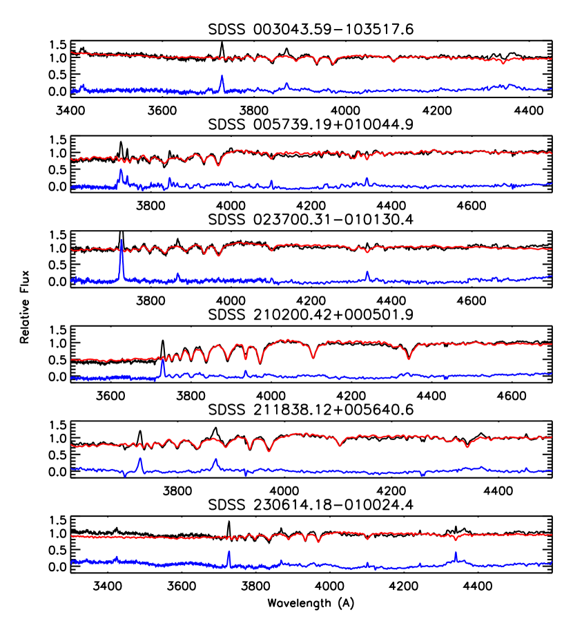
Figure 2.— Spectral fitting results. The data are plotted in black, the best fit model in red, and the redsidual is plotted in blue. Each spectrum is plotted in the rest frame.

We obtained an additional longer wavelength spectrum that extends to rest frame 5800 Å for the object SDSS $0237-0101$. We fit the spectral region around Mg IB with the expectation that features from the underlying older stellar population would be dominant in this region. The exact region was from $5020-5550$ Å with one emission line at 5198 Å blocked from the fit. Fitting this region can be complicated due to [Mg/Fe] correlation with velocity dispersion (Jørgensen et al., 1999; Wold et al., 2007). However, we found identical results between fits conducted with and without the Mg IB absorption blocked from the fit. Despite some effort in matching the templates to the host galaxy and using various weighting schemes, we were unable to derive a robust measure of $\sigma_{*}$ from this region. The best fit dispersion using this region was 155 (+19, $-$18) km s^-1, which is smaller than the dispersion measured from the Balmer region, i.e., 214 (+19, $-$5) km s^-1). However, we were able to fit $\sigma_{*}$ values that ranged from $\sim 145\sim 210$ km s^-1 while still maintaining visually similar fits. In Figure 3, we show example fits for this region using $\sigma_{*}$ values of 145 km s^-1, 175 km s^-1, and 210 km s^-1. As in Figure 2, the data are plotted in black, and the models are plotted in red. The residuals for the three fits shown are similar to one another. These fits indicate that there are likely model degeneracies that are affecting the determination of $\sigma_{*}$ in this region.

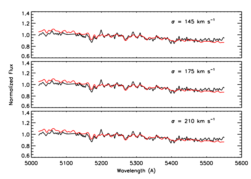
Figure 3.— Spectral fitting results for the Mg IB region of SDSS $0237-0101$. We have plotted the best fits for three values of $\sigma_{*}$: 145, 175, and 210 km ^-1. The data are plotted in black, the best fit model in red.

4. Black Hole Mass

Black hole masses can be estimated using the virial method under the assumption that the broad line region (BLR) gas is virialized. To calculate the virial parameter, we require measurements of the gas velocity and orbital radius. The velocity is, in principle, easily measured from broad line widths (e.g., Mg II, H$\beta$, H$\alpha$). Furthermore, reverberation mapping studies have shown a correlation between the radius of the BLR (R_BLR) and the continuum luminosity of the active nucleus (Kaspi et al., 2000; Bentz et al., 2009a). Thus, the observables to employ the virial method are the line width and continuum luminosity.

To convert the virial parameter ($VP=R_{\rm BLR}\Delta v^{2}/G$) to a black hole mass, one must include an additional f-factor, which accounts for unknown geometries in the broad line region. Woo et al. (2010) have measured this factor by scaling the virial parameter of reverberation mapped AGN to match the M${}_{\rm BH}-\sigma_{*}$ relation, and found f $=5.2$. This is consistent with values found by previous authors (Onken et al., 2004) that are about 1.8 times higher than an f-factor assuming an isotropic BLR velocity field.

In the following sections we describe how we measured the broad line widths and continuum luminosities used in the virial black hole mass calculation. We measure the H$\alpha$ FWHM, and the Mg II $\lambda\lambda 2796,2803$ FWHM to use as BLR gas velocities. We measure the 5100 Å AGN continuum luminosity to use as a proxy for the BLR radius. In the following we will refer to $\lambda$L_λ as L₃₀₀₀ or L₅₁₀₀ for $\lambda=3000$ Å and $\lambda=5100$ Å, respectively. Table 4 displays the relevant measurements. Table 5 shows the mass estimates and Eddington ratios.

Table 4Line Widths and Monochromatic Luminosities

		H$\alpha$	Mg II		L3000	L5100
N	Object	FWHM	$\sigma_{intr}$	FWHMintr	3000 Å	5100 Å
1	SDSS $003043.59-103517.6$	4981 $\pm$ 428	1563	3066	4.7${}^{+1.7}_{-1.2}$	1.5${}^{+0.6}_{-0.4}$
2	SDSS $005739.19+010044.9$	4300 $\pm$ 210	1871	3464	0.36${}^{+0.07}_{-0.06}$	0.30${}^{+0.08}_{-0.06}$
3	SDSS $023700.31-010130.4$	7125 $\pm$ 770	2357	4855	0.39${}^{+0.2}_{-0.1}$	0.41${}^{+0.2}_{-0.1}$
4	SDSS $210200.42+000501.9$	6132 $\pm$ 315	$\cdots$	$\cdots$	0.58${}^{+0.08}_{-0.07}$	0.79${}^{+0.06}_{-0.06}$
5	SDSS $211838.12+005640.6$	6303 $\pm$ 501	2278	2913	1.4${}^{+0.4}_{-0.3}$	1.7${}^{+0.3}_{-0.5}$
6	SDSS $230614.18-010024.4$	3704 $\pm$ 719	1857	2468	1.1${}^{+0.7}_{-0.4}$	1.2${}^{+1.2}_{-0.4}$

4.1. H$\alpha$

The H$\beta$ broad emission line is often used to calculate black hole masses in single-epoch spectra of AGN. However, in our sample, the absorption-line spectrum of the host galaxy can significantly contaminate the H$\beta$ emission line. Often the broad H$\beta$ line is completely unobserved, so H$\beta$ emission is not suitable for measuring M_BH. On the other hand, H$\alpha$ is much less affected by the stellar absorption line than H$\beta$, and broad H$\alpha$ is always observed in the spectra of the targets.

To calculate black hole masses we adopt the relation from Greene et al. (2010a):

$${\rm M_{BH}}=(9.7\pm 0.5){\sf x}10^{6}(\frac{\rm{L_{5100}}}{10^{44}{\rm~{}erg~{}s^{-1}}})^{0.519\pm 0.07}$$

$${\sf x}(\frac{{\rm FWHM_{H\alpha}}}{10^{3}~{}{\rm km~{}s^{-1}}})^{2.06\pm 0.06}~{}{\rm M_{\odot}}$$ (2)

Greene et al. use a virial coefficient from Onken et al. (2004) (f$=5.5$), which is 1.8 times higher than the assumption of isotropic random motions. Their equation was originally determined by Greene & Ho (2005), who derive a conversion between H$\alpha$ and H$\beta$ FWHM. Thus, the above equation converts the H$\alpha$ FWHM to that of H$\beta$, and uses an f-factor appropriate for H$\beta$.

Woo et al. (2010) measure the M${}_{\rm BH}-\sigma_{*}$ relation for the reverberation mapped sample of the Lick AGN Monitoring Project (Walsh et al., 2009; Bentz et al., 2009b, 2010). Woo et al. determine the geometric factor for f$=5.2^{+1.2}_{-1.3}$ by scaling the determined H$\beta$ virial products to the local M${}_{\rm BH}-\sigma_{*}$ relation for inactive galaxies determined by Gültekin et al. (2009). Because the relation from Greene et al. (2010a) uses the same virial coefficient as found by Woo et al., any differences we find between our sample and that of Woo et al. will not be due to differences between f-factors.

To measure the widths of the H$\alpha$ broad emission line we used the task specfit in the STSDAS package of IRAF (Kriss, 1994). Our LRIS spectroscopy does not cover the H$\alpha$ region, so we measure the width from the SDSS spectra (DR7; Abazajian et al., 2009). The task specfit minimizes the $\chi^{2}$ using a simplex method and returns the central wavelength, integrated flux, FWHM, and skew of each line. We fit the region from 6400 - 6700 Å using five components: a power law continuum, three Gaussians for the narrow line components of [N II] $\lambda$6548, H$\alpha$, and [N II] $\lambda$6583, and an additional Gaussian for the H$\alpha$ broad emission line. We held the relative positions of the [N II] lines constant for the fitting procedure, and constrained all the Gausians to be symmetric. We fit a narrow line model using [O III] 5007 on objects where the line was visible and scaled the model to the [N II] and H$\alpha$ narrow lines. The specfit task also returns errors on the fitted parameters, which are generally large due to the resolution and S/N of the SDSS spectra. We show the fits of the H$\alpha$ region for all objects in Fig. 4.

The stellar H$\alpha$ absorption line from the host galaxy is small compared to each of these components, and significantly more narrow than the broad emission line of the active nucleus. Using spectra and host galaxy fits for PSQs from Cales et al. (2012, (in preparation)) that cover H$\alpha$, we determined that the host galaxy absorption component does not affect the measurement of the broad line FWHM.

The data of Cales et al. (2012, (in preparation)) cover the H$\alpha$ region for the object SDSS $0057+0100$, and have higher resolution and S/N ($\sim$28 pix^-1 on the continuum) than the SDSS spectrum (S/N$\sim$10 pix^-1 on the continuum). Following the same procedure, the FWHM measured using these data agrees within the errors of the FWHM measured from the SDSS spectrum. We adopt the width measured with the data from Cales et al., because the S/N is an improvement over the SDSS spectrum.

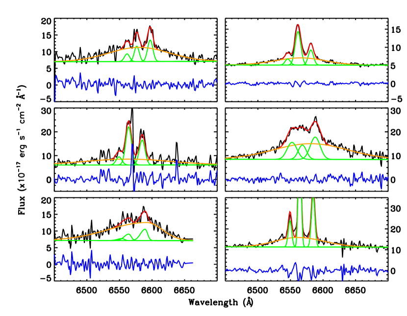
Figure 4.— Broad- and narrow-line decompositions of the H$\alpha$ region. The SDSS DR7 spectra are plotted in the restframe in black. The models of the narrow emission lines and continuum are plotted in green, and the H$\alpha$ broad emission line component is plotted in orange. The overall fit is plotted in red. The residuals are plotted in blue. The objects in the left column from top to bottom are $0030-1035$, $0237-0101$, and $2118+0056$. The objects on the right are $0057+0100$, $2102+0005$, and $2306-0100$.

4.2. Mg II

As with the H$\alpha$ emission line, there are several prescriptions for calculating black hole masses from the Mg II $\lambda\lambda 2796,2803$ broad emission doublet (McLure & Jarvis, 2002; McGill et al., 2008; Rafiee & Hall, 2011; Vestergaard & Osmer, 2009). Of these, the calibration from Vestergaard & Osmer (2009) is based on the largest number of objects and is calibrated with L₅₁₀₀ in addition to other continuum luminosities. As described in the next section, we consider the 5100 Å continuum luminosity to be better constrained than the 3000 Å luminosity, which is typically used in conjunction with the Mg II emission to calculate black hole masses. The formulation that we adopt from Vestergaard & Osmer is:

$${\rm M_{BH}}=10^{6.96}(\frac{{\rm FWHM_{MgII}}}{1000{\rm kms^{-1}}})^{2}(\frac{\rm{L_{5100}}}{10^{44}{\rm ergs^{-1}}})^{0.5}~{}{\rm M_{\odot}}$$ (3)

According to Vestergaard & Osmer, the uncertainty in the zero point of this relation is 0.55 dex. This is the dominant factor in the uncertainty on the black hole mass calculated from the Mg II emission.

To measure the Mg II width, we first fitted and subtracted an Fe II emission template from the spectrum. Iron emission can contaminate the flux surrounding the Mg II emission and affect the measurement of the broad line width. We used the template from Vestergaard & Wilkes (2001), who derived the template from the observed spectrum of the narrow-line Seyfert 1 galaxy I Zw 1.

The template by Vestergaard & Wilkes (2001) only includes Fe emission that may contaminate the wings of the Mg II profile. To account for Fe emission that may contaminate the core of the line, Fine et al. (2008) and Kurk et al. (2007) add a constant flux under the Mg II core equal to 20% of the average Fe flux at $2930-2970$ Å. This is based on the theoretical Fe emission models of Sigut & Pradhan (2003). To determine if the theoretical flux may have affected our Mg II width measurements, we subtracted the additional flux from the fit of SDSS $0237-0101$ and re-measured the width of the Mg II emission. There was no difference measured between the two methods, so we do not believe this small amount of theoretical flux has affected the measurements of Mg II widths.

We used a fitting routine similar to the one that we used to determine stellar velocity dispersions to scale and broaden the Fe template before subtraction. The main differences between the way that we modeled the Balmer region and the Mg II region are that we replaced the host galaxy stellar template with the Fe template from Vestergaard & Wilkes (2001) and the fitted continuum includes contributions from both the active nucleus and host galaxy at these wavelengths. We adopted a power law to fit the continuum, as we expect that the host galaxy contribution to the flux at these wavelengths is comparatively small. We fit a total of five parameters: normalization and slope for a power law continuum, and the scaling constant, velocity dispersion ($\sigma_{Fe}$), and velocity offset for the Fe template.

We first estimated the continuum from a region relatively uncontaminated by Fe emission: $3010-3026$ Å. The result was used as the continuum initial estimate for the main fitting routine. The Fe template does not include the Mg II emission line, so we blocked the feature from contributing to the $\chi^{2}$ during the minimization. This region varied in size for each object depending on the strength of the emission. We allowed $\sigma_{Fe}$ to vary up to $2000$ km s^-1, but each fit produced a value smaller than 1000 km s^-1. The best fit model was then subtracted from the spectrum leaving a residual spectrum. We show Fe template fits to all objects in Fig. 5.

Objects SDSS $0057+0100$ and SDSS $2102+0005$ were peculiar, and were not fit well by the Fe template (first and second object on the right side of Fig. 5). The spectrum of SDSS $0057+0100$ shows some signs of absorption to the blue side of Mg II. However, the noise significantly increases at the edge of the spectrum, making the continuum level difficult to determine. It is possible that SDSS 0057+0100 is a low-ionization broad absorption line (LoBAL) quasar, but without a clear determination of the continuum level at shorter wavelengths, we hesitate to classify it as such. In order to fit the Fe template to this object, we blocked the wavelength region shortward of and including the Mg II emission ($<$ 2840 Å) from the fit, allowing the overall fit to be determined by the longer wavelengths. Then we subtracted the entire fitted spectrum from the region before measuring the Mg II width. The spectrum of SDSS $2102+0005$ has better S/N on the blue side of Mg II than that of SDSS $0057+0100$, and the profile of Mg II makes it clear that the object is a LoBAL. Because the spectrum shows strong absorption over the blue wing of the Mg II line, we were unable to reliably measure a Mg II line width. We do not report a Mg II width measurement for SDSS $2102+0005$, but do include one for SDSS $0057+0100$.

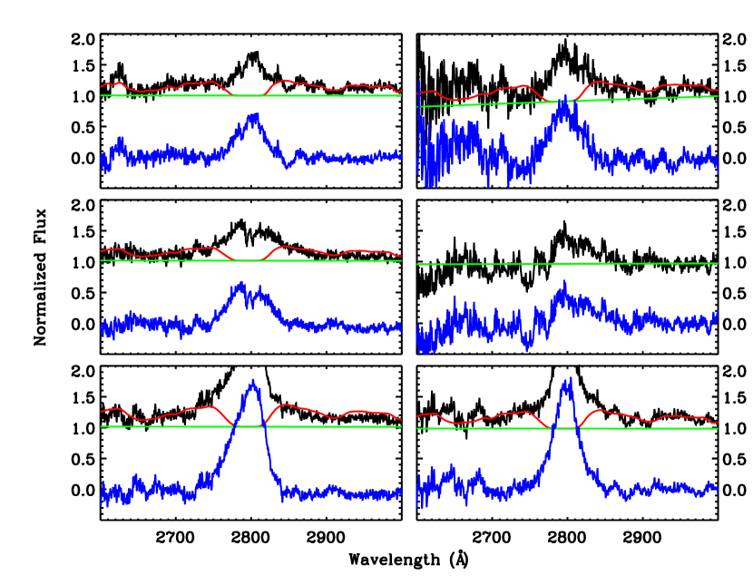
Figure 5.— Fe template fitting in the Mg II region. The LRIS data are plotted in black. The overall fitted Fe template is plotted in red, and the continuum is plotted in green. The residual spectrum (data - model) is plotted in blue. The objects are in the same order as Fig. 4

4.3. Continuum Luminosities

The continuum luminosity is used as a proxy for the BLR radius in the virial method to measure black hole mass. We measure the continuum luminosity from the power-law continuum of our model. The power-law is multiplied by a Legendre polynomial to simulate reddening effects and non-stellar emission, and the product of the continuum and Legendre polynomial represents the reddened nucleus free of host contamination. In order to obtain the intrinsic continuum luminosities we follow a two step process: First, we calculate a scaling factor between the product of the continuum and Legendre polynomial fitted by our spectral code and the $HST$ F606W photometry of the nucleus, which has been deconvolved from the host galaxy (Cales et al., 2011). The scale factor effectively flux calibrates our fitted spectrum to the $HST$ photometry. Then we apply the scaling factor to the fitted underlying power law continuum (without the Legendre polynomial).

We measure the monochromatic luminosities from the scaled power law. It is important to note that both 3000 Å and 5100 Å fall outside the spectral region that we modeled. Thus, the luminosites are extrapolations from our fitted quasar power-law continuum. We define uncertainty on the continuum luminosities by varying the slope of our intrinsic continuum by $\pm$0.1, which is the scatter in the average quasar spectral slope (Vanden Berk et al., 2001). The emission at 3000 Å has contributions from the active nucleus, the host galaxy, and iron. While we have a template that models the iron emission (Vestergaard & Wilkes, 2001), attempting to separate the three components would include many free parameters and model degeneracies may become a significant issue. Furthermore, the photometry that we use to scale the fitted active nucleus spectrum is in the observed $HST$ F606W filter. Because 5100 Å is much closer to both our spectral fitting region and the F606W photometry, we consider L₅₁₀₀ to be much better constrained than L₃₀₀₀. We present both measured luminosities and their formal uncertainties in Table 4. The true uncertainty for the L₃₀₀₀ measurement is larger than the formal uncertainty that we have reported for the reasons noted above.

5. Results

In the previous sections we have presented our $\sigma_{*}$ and M_BH measurements of six PSQs. We now examine the relationship between the black holes and their host bulges through the M${}_{\rm BH}-\sigma_{*}$ and M${}_{\rm BH}-$L_bulge relations. We further examine the properties of the host galaxy bulges with the Faber-Jackson relation to determine if the bulges are dynamically peculiar compared to evolved systems in the local universe. By examining these three relations, we can determine if any observed offset is primarily due to over/under-massive BHs or dynamically perturbed bulges.

Using the H$\alpha$ and Mg II emission line widths, we calculated masses of the black holes in six post-starburst quasars and present the values in Table 5. In five of the six objects, we measure larger masses based on the H$\alpha$ broad line than the Mg II broad line. We were unable to measure the M_BH based on the Mg II broad line for SDSS $2102+0005$, because the line profile for this object is affected by an absorption trough on the blue wing, as described above.

The relations from Greene et al. (2010a) and Vestergaard & Osmer (2009) are each calibrated to H$\beta$. In principle they should give consistent results, because the two prescriptions are measuring the same black hole mass, and both H$\alpha$ and Mg II should be reliable indicators of the BLR gas dynamics and M_BH. That is, according to Greene & Ho (2005), the correlation between the H$\alpha$ FWHM and the H$\beta$ FWHM has a scatter on the order of $\sim 0.1$ dex. Furthermore, Vestergaard & Osmer (2009) report their calibration produces Mg II-based masses that are consistent with the H$\beta$ and C IV-based masses within $\sim 0.1$ dex. However, the 1$\sigma$ scatter on the zero point of the Vestergaard & Osmer relation is 0.55 dex. If we consider this large error associated with the Mg II-based calculation, then our calculated H$\alpha$ and Mg II masses are consistent. The discrepancy could arise if, at least for PSQs, the geometric f-factor were different between the emission line gas species. This is not unlikely, as magnesium has a lower ionization potential than hydrogen, and may arise from a different location within the BLR.

Table 5Black Hole Masses

		MBH	MBH	Lbol/LEdd	Lbol/LEdd
N	Object	H$\alpha$	Mg II	5100 Å	[O III]
1	SDSS $003043.59-103517.6$	3.25${}^{+3.0}_{-1.5}$	1.1	0.037	0.019
2	SDSS $005739.19+010044.9$	1.06${}^{+1.1}_{-0.5}$	0.60	0.023	0.076
3	SDSS $023700.31-010130.4$	3.49${}^{+4.0}_{-1.8}$	1.4	0.009	0.057
4	SDSS $210200.42+000501.9$	3.59${}^{+3.2}_{-1.7}$	$\cdots$	0.018	0.013
5	SDSS $211838.12+005640.6$	5.70${}^{+5.0}_{-2.6}$	1.0	0.024	0.027
6	SDSS $230614.18-010024.4$	1.56${}^{+1.9}_{-0.8}$	0.60	0.060	0.062

5.1. The M${}_{\rm BH}-\sigma_{*}$ Relation

We have plotted the objects studied here on the M${}_{\rm BH}-\sigma_{*}$ diagram (Fig. 6). For comparison we present the relation measured by McConnell et al. (2011a), who update the plot with compiled measurements from the literature. We also include reverberation mapped AGN from Woo et al. (2010). The best fit from McConnell et al. is plotted as a dot-dashed line, and the fit from Woo et al. is plotted as the dashed line. We plot the H$\alpha$ based black hole masses in red triangles. The scatter reported by both McConnell et al. and Woo et al. is $\sim 0.43$ dex, and the H$\alpha$ based M_BH all fall within or above this scatter with respect to either relation. Three of the black hole masses that were based on the Mg II measurement are consistent with this scatter.

The objects SDSS $0030-1035$ and SDSS $2306-0100$ appear significantly offset from the M${}_{\rm BH}-\sigma_{*}$ relation. Both of these galaxies were classified by Cales et al. (2012) as face-on disks. The face-on disk presents a dynamically cold stellar component with small line-of-sight velocity dispersion, and Bennert et al. (2011) showed that this orientation can bias the measured velocity dispersion toward smaller values. The sample of Woo et al. (2006) contains four face-on disks, and the objects do have lower $\sigma_{*}$ values than the remainder of their sample. However, the magnitude of the bias for their objects is only $\sim 30-50$ km s^-1 ($\Delta$$\sigma_{*}$ $\sim 0.1$ dex), whereas the two objects here have offsets on the order of $\sim 140$ km s^-1 ($\Delta$$\sigma_{*}$ $\sim 0.6$ dex). Furthermore, as we show below, one of these objects is consistent with the Faber-Jackson relation.

One other object in our sample was classified by Cales et al. (2012) as a face-on disk (SDSS $0057+0100$), but it falls within the scatter of the M${}_{\rm BH}-\sigma_{*}$ relation. SDSS $0237-0101$ also has a bulge+disk morphology, but is not face-on and falls within the scatter of the M${}_{\rm BH}-\sigma_{*}$ relation. The last two objects (SDSS $2102+0005$ and SDSS $2118+0056$) are dominated by bulges and fall outside the defined 1$\sigma$ scatter of the M${}_{\rm BH}-\sigma_{*}$ relation.

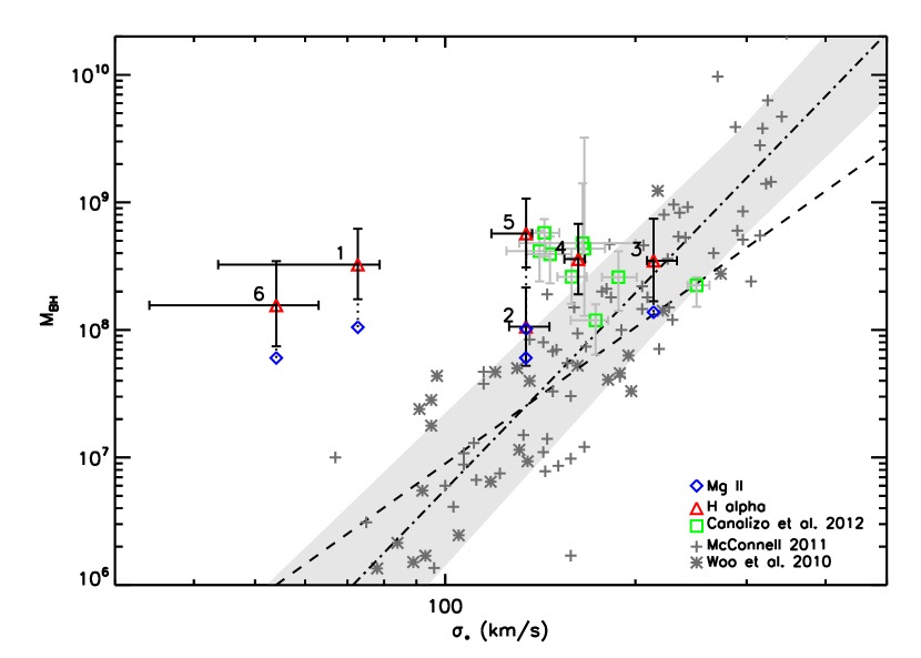
Figure 6.— Plot of our objects compared to the locally-defined M${}_{\rm BH}-\sigma_{*}$ relation. The relation by McConnell et al. (2011a) is plotted as a dot-dashed line and grey plus symbols. The scatter is shown as a shaded grey region.The relation of reverberation mapped active galaxies by Woo et al. (2010) is plotted as a dashed line with grey asterisks. We plot the red quasars from Canalizo et al. (2012) in green squares. The black hole masses of the PSQs based on H$\alpha$ and Mg II are plotted as red triangles and blue diamonds, respectively.

In Fig. 7 we show the offset of M_BH (top panel) and the offset of $\sigma_{*}$ (bottom panel) from the relation defined by Woo et al. (2010) as a function of $z$. Previous studies have found an offset from the local M${}_{\rm BH}-\sigma_{*}$ relation, including Woo et al. (2006, 2008) and Canalizo et al. (2012). The objects in our sample span a redshift range that overlaps with the samples of Canalizo et al. and Woo et al.. Furthermore, the trends seen by them appear to continue in our objects. As discussed by Canalizo et al., at first glance this implies very recent evolution in the M${}_{\rm BH}-\sigma_{*}$ relation.

The average M_BH offset for the sample of all six quasars with respect to the relation by Woo et al. (2010) is 1.25 dex when determined from the H$\alpha$ broad line. If we exclude the object that does not conform to the Faber-Jackson relation (SDSS $2306-0100$, see below), then the average offset in M_BH becomes 1.06 dex. This result is significantly higher than the scatter in the local M${}_{\rm BH}-\sigma_{*}$ relation, which is $\sim 0.43$ according to both Woo et al. (2010) and McConnell et al. (2011a). The offset we measure is slightly larger than the average offsets of red quasars found by Canalizo et al. (2012) and of non-local Sy 1s from Woo et al. (2006, 2008). Note also that the Mg II-based black hole masses are systematically lower than the H$\alpha$ based masses. The average M_BH offset, again excluding SDSS $2306-0100$, based on the Mg II measurements is only 0.64 dex. The small number of objects in our sample preclude us from claiming whether the entire sample of PSQs is on average offset from the local M${}_{\rm BH}-\sigma_{*}$ relation. To determine that, we will need to study more objects from the parent sample of PSQs. Furthermore, it is not unreasonable that for these six objects we will find some that fall above the 1$\sigma$ scatter of the local relation, but it is curious that all of the offsets are on the same side of the relation.

The issue is complicated by the matter of the discrepancy between black hole masses measured with the Mg II and with the H$\alpha$ emission lines. We used the SDSS data to measure the H$\alpha$ emission for all but one object, and the SDSS spectroscopy has low S/N ($<10$ pix^-1). Denney et al. (2009) show that using a Gauss-Hermite polynomial to fit low S/N data may overestimate the FWHM of the H$\beta$ line. In the one object for which we have high S/N LRIS spectroscopy (SDSS $0057+0100$) of the H$\alpha$ region, we measured a lower FWHM of the H$\alpha$ broad line compared to the SDSS spectrum. The difference was $\sim 400$ km s^-1 ($\sim 8\%$). The black hole mass for SDSS $0057+0100$ using the larger width is only a factor of 1.2 greater than using the smaller width, which is within our defined errors. Smaller H$\alpha$ widths would bring the H$\alpha$-based mass measurements closer to the Mg II-based measurements. However, this small effect is unlikely to reconcile the two measurements. As an alternative explanation, it is possible there is a systematic difference in BLR gas dynamics between the H$\alpha$ and Mg II-emitting gas.

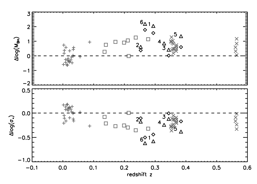
Figure 7.— The offset from the local M${}_{\rm BH}-\sigma_{*}$ relation (Woo et al., 2010) is plotted against the redshift of the objects. The PSQs from our sample are plotted twice with triangles representing the H$\alpha$-based M_BH measurement and the diamonds the Mg II-based measurement (same as Fig. 6). The red quasars of Canalizo et al. (2012) are plotted as squares, and the Seyfert 1 galaxies from Woo et al. (2006) and Woo et al. (2008) are plotted as X symbols. The objects that define the local relation from Woo et al. (2010) are plotted as plus symbols.

5.2. The M${}_{\rm BH}-$L_bulge Relation

We plot the M${}_{\rm BH}-$L_bulge relation in Fig. 8. This serves as a test of the bulge properties of the host. If the objects follow this relation, then the black holes of these galaxies may be “normal” for their bulges, while the velocity dispersions cause the offset seen in the M${}_{\rm BH}-\sigma_{*}$ relation. In order to compare the bulge luminosities that we have measured here to measurements of systems in the local universe, we need to account for the change in luminosity associated with the evolution of stellar populations.

We measured the bulge luminosities in a procedure that is similar to the measurement of the AGN continuum luminosities. For each object, we scaled our fitted host galaxy template to the measured bulge photometry of Cales et al. (2011) in the $HST$ F606W filter. We then measure V band photometry from the scaled host spectrum. Photometry from Cales et al. has already been k-corrected, but we also apply a passive evolution correction using the online calculator of van Dokkum & Franx (2001). We applied the “Default 1: single stellar population” setting using the calculator, which uses a burst of star formation that passively evolves. This setting approximates the starburst event of our PSQs, which have luminosities dominated by the young population (see Table 3).

The “Default 1” setting of the passive evolution calculator assumes that the stars were formed at redshift $z>>1$. However, the PSQs clearly have had a recent starburst within the past $\leq 1$ Gyr. Thus, we adjusted this parameter to more closely match the star formation history of our targets. The difference in redshift from 0.3 (the average of the sample) to 0.4 corresponds to roughly 840 Myr. This is appropriate for all of our targets except SDSS $2118+0056$, which has a redshift closer to 0.4 than 0.3. For this target we adopt the passive evolution correction assuming a formation redshift of 0.5 (a 740 Myr stellar population). As expected, this produced a larger correction than assuming all stars formed at $z>>1$, and applying this correction shifts the objects to smaller V band luminosities. We adopt an error on the bulge luminosities that assumes 0.1 mag error from the fits of Cales et al. and an additional 10% error on the spectral host-AGN decomposition.

In Fig. 8, the solid line shows the best fit relation from McConnell et al. (2011a), who compile measurements of individual galaxies from the literature, including brightest cluster galaxies. The two dotted lines show fits defined by the uncertainty in their scaling and slope, while the grey shaded region shows the intrinsic scatter they measured. Two of the H$\alpha$-based black hole mass measurements (triangles) fall above the scatter in the relation, while the remaining objects are consistent with the relation. However, if we consider the Mg II-based black hole masses (diamonds), all of the objects fall on the relation. We also note that the scatter from McConnell et al. (0.5 dex) is somewhat greater than that of Gültekin et al. (2009), who found 0.38 dex. If we were to consider the fit from Gultekin et al., four of the H$\alpha$-based black hole masses would fall above the relation. Thus, to some degree, the interpretation of the offset from the relation depends on the relation’s true intrinsic scatter.

The result is quite similar to that from the M${}_{\rm BH}-\sigma_{*}$ relation. That is: PSQs fall within the scatter or above the M${}_{\rm BH}-$L_bulge relation if we consider the black hole masses measured from H$\alpha$. Whereas, if we consider the M_BH measured from Mg II, the PSQs are consistent with the relation. From this we can surmise that if the offset is to be believed, the black holes really are over-massive for their bulges.

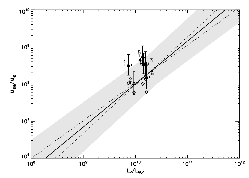
Figure 8.— The M${}_{\rm BH}-$L_bulgerelation. The solid line is the relation from McConnell et al. (2011a). The dotted lines show the relations defined by the uncertainty in the fitted scale and slope with scatter shown as the grey shaded region ($\pm$0.5 dex). H$\alpha$ based black hole masses of the PSQs are plotted as triangles, and the Mg II based masses of the same objects are plotted as diamonds.

5.3. The Faber-Jackson Relation

Figure 9 shows the location of our sample on the Faber-Jackson relation (Faber & Jackson, 1976). If the $\sigma_{*}$ values that we measured are causing the offset seen from the M${}_{\rm BH}-\sigma_{*}$ relation, we expect the objects to fall below this relation. That is, the objects should have velocity dispersions that are too small for their bulge luminosities. This is the case for one object, but the remaining five are generally consistent with the relation.

The left and right panels show the SDSS $g$ band and $r$ band absolute AB magnitude, respectively. The $g$ and $r$ photometry were measured with the same method that we used to measure the V band luminosity (see previous section) with the additional step of converting luminosities into SDSS AB magnitudes for ease of comparison. This also required transforming the passive evolution corrections from B and V to $g$ and $r$ corrections, for which we used the relations from Jester et al. (2005). Nigoche-Netro et al. (2010) calculate the Faber-Jackson relation in discrete magnitude bins of width 1 magnitude. Considering the $g$ absolute magnitudes (left panel), the PSQs appear to follow the relations defined by Nigoche-Netro et al.. The dashed line represents the relation appropriate for objects with magnitudes between $-19.5$ and $-20.5$. Two objects fall in the magnitude bin $-18.5$ to $-19.5$ and are consistent with that relation. The only object that falls significantly offset is SDSS 2306-0100, which is one of the face-on disk galaxies. Considering the $r$ magnitudes (right panel), all objects fall in the magnitude bin $-20>M_{r}>-21$. Five objects are consistent with the relation, while SDSS 2306-0100 is again significantly offset. In both panels we have plotted the overall relation using the entire sample of Nigoche-Netro et al.. The fit for their overall sample has an intrinsic dispersion of 0.6 dex.

Desroches et al. (2007) have also studied the luminosity dependence of the Faber-Jackson relation. They derive a quadratic fit to to the relation in the SDSS $r$ band using data from the NYU Value Added Galaxy Catalog (Blanton et al., 2005). While Nigoche-Netro et al. (2010) use only galaxies that are well fit by a de Vaucouleurs profile and the corresponding magnitudes, Desroches et al. (2007) select objects with a range of Sérsic indices and calculate a “Sérsic-like” magnitude from a Petrosian magnitude. As Desroches et al. explain, the Sérsic index is correlated with the galaxy luminosity and therefore may bias the slope of the relation if not accounted for. We have plotted the quadratic fit from Desroches et al. log $\sigma_{*}$ $=-1.79+0.674$(log L)$-0.0234$(log L)²; M$=-2.5$(log L)) with 0.1 dex scatter in the right panel of Fig. 9 (solid line and dark grey shading) along with the fit from Nigoche-Netro et al. (2010). Three of our objects fall on the relation derived by Desroches et al.. One object falls above the relation (within 2$\sigma$), while two fall significantly below the relation. The two objects that are significantly offset are also the most offset from the M${}_{\rm BH}-\sigma_{*}$ relation, suggesting that at least part of the offset is due to peculiar dynamics of the stellar population.

Norton et al. (2001) studied the velocity dispersions of quiescent E+A galaxies. To separate the post-starburst population from the underlying older population of stars they simultaneously fit the 4100 - 5250 Å region with K, G, and A star templates. They find that the post-starburst population does not show a significant correlation between its velocity dispersions and the overall host luminosities. However, the distribution of dispersions for their sample is consistent with the Faber-Jackson relation using data from Faber et al. (1989) and Jorgensen & Franx (1994). The older stellar population $\sigma_{*}$ does show correlation with host luminosity, but the objects fall on average $\sim$0.6 mag brighter than the elliptical galaxies of similar dispersion. We do not separate the post-starburst population from the older population with unique measures of $\sigma_{*}$ as Norton et al. do, so the value of $\sigma_{*}$ that we measure has influence from both populations.

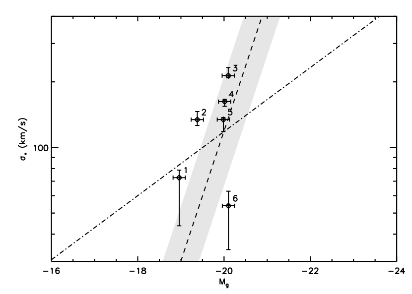
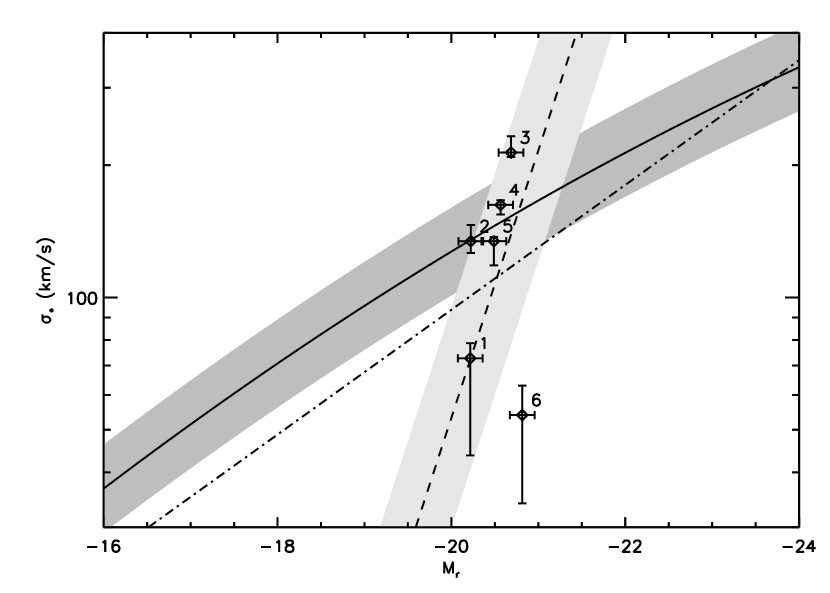
Figure 9.— The Faber-Jackson relation. Left: The SDSS $g$ band absolute AB magnitudes. The dashed line is the best fit from Nigoche-Netro et al. (2010) for the magnitude bin -19.5 $>g>$ -20.5. Right: The SDSS $r$ band absolute AB magnitudes. The dashed line is the best fit from Nigoche-Netro et al. (2010) for the magnitude bin -20 $>r>$ -21. The solid line and dark grey region show the quadratic fit and scatter to the Faber-Jackson relation from Desroches et al. (2007). For both panels the the light grey shaded region shows the scatter in the fit from Nigoche-Netro et al. ($\pm$0.25 dex, 2010), and the dot-dashed line shows the best fit for the overall sample of Nigoche-Netro et al..

6. Discussion

We have measured M_BH and $\sigma_{*}$ in six AGN that are hosted by galaxies showing post-starburst stellar populations (“post-starburst quasars”). These objects fall on or above the locally defined M${}_{\rm BH}-\sigma_{*}$ and M${}_{\rm BH}-$L_bulge relations. The location of the PSQs on the M${}_{\rm BH}-\sigma_{*}$ diagram is consistent with other studies of objects at $z>0.1$ (Canalizo et al., 2012; Woo et al., 2008, 2006).

We have used the Balmer region, which includes the Balmer series, Ca lines, the G band, and other stellar features to estimate the stellar velocity dispersions. While we have used host galaxy templates that approximate the stellar population of the host galaxies, it is possible that the young and old populations have different velocity dispersions. The kinematics of the young population are influenced by the mechanism that triggered the starburst. In a theoretical work, Bekki et al. (2005) describe various models of galaxy interactions (major/minor mergers, strong tidal interactions, etc.) that lead to E+A spectral signatures. They find a range of morphologies, velocity dispersions, and starburst mass fractions resulting from the merger event depending on the specific model used. The kinematic properties of the resulting post-starburst population depend on the initial parameters of the galaxy-galaxy interaction that induces the starburst.

The morphologies presented by Cales et al. (2011) for our sample indicate that these objects have only minorly disturbed features, if any, that could indicate a recent merger event. Four objects of our sample are described by Cales et al. as containing a disk component. However, the overall sample of PSQs display a range of morphologies, and Cales et al. found that half of the observed sample appear to be post-merger remnants. The variety of morphologies seen in the parent sample is consistent with the simulations conducted by Bekki et al. (2005), indicating a range of possible galaxy-galaxy interactions that trigger the starburst event (e.g., tidal interactions, minor/major mergers). Regardless of the triggering mechanism, the PSQs, at least in this subsample, have M_BH and $\sigma_{*}$ that are generally consistent with previously studied $z>0.1$ galaxies.

The origin of the velocity dispersion (pressure supported versus rotational) should influence whether the objects fall on the M${}_{\rm BH}-\sigma_{*}$ relation, which is best defined for pressure supported bulges. Observationally, Norton et al. (2001) studied the young and old populations independently in E+A galaxies and found them to be largely pressure supported, with the younger post-starburst population having higher $\sigma_{*}$ than the old population. However, Bekki et al. (2005) had trouble reproducing this result with their models. By contrast, Pracy et al. (2009) found rotation to play a dominant role in their studied E+As.

We do not separate the young and old populations in our analysis, so the kinematical differences between the post-starburst population and older population in PSQs remains a question. In principle, we could adopt an additional free parameter in our model to measure the velocity dispersion of the old population separately from the young population. However, this would introduce degeneracies that would be difficult to disentangle, especially with the presence of the active nucleus. We are currently conducting an investigation into the kinematic differences between young and old populations in quiescent E+A galaxies that lack the active nucleus continuum contamination (Hiner & Canalizo, 2012, in preparation). This analysis will be similar to that of Norton et al., but we will include multiple wavelength regions. By including longer wavelength regions, such as the Mg IB and Ca II triplet regions, we will be able to further distinguish between the young and old stellar populations.

We have also measured the bulge luminosities of the host galaxies. After plotting the M${}_{\rm BH}-$L_bulge and Faber-Jackson relations, we find a scenario which rules out $\sigma_{*}$ bias as the source of the offset from the M${}_{\rm BH}-\sigma_{*}$ relation for three of the six objects we measured. Two objects (SDSS $0030-1035$ and SDSS $2306-0100$) are significantly offset from the M${}_{\rm BH}-\sigma_{*}$ relation. SDSS $2306-0100$ is additionally offset from the Faber-Jackson relation, indicating that the measured $\sigma_{*}$ may be significantly influenced by the face-on disk of the host galaxy. SDSS $0030-1035$ is consistent with the relation as defined by Nigoche-Netro et al. (2010), but it falls significantly below that of Desroches et al. (2007), so it may also be influenced by the face-on disk. While SDSS $0237-0101$ falls above the Desroches et al. Faber-Jackson relation by less than 2$\sigma$, it is also the object that falls closest to the best fit M${}_{\rm BH}-\sigma_{*}$ relation. A reduction of $\sim 50$ km s^-1 in $\sigma_{*}$ would bring it in line with the Desroches et al. fit, but drive the object left of the M${}_{\rm BH}-\sigma_{*}$ relation (consistent with the other offsets). Peculiar dynamics can clearly influence the measured velocity dispersion, and with a more statistically significant sample, the general trends will become more apparent.

The offset from the M${}_{\rm BH}-\sigma_{*}$ relation is consistent with that found by Canalizo et al. (2012). Similar to their sample and the samples of Woo et al. (2006) and Woo et al. (2008), the black holes measured here all have masses $\geq 10^{8}$ M_⊙. This brings up the question of sample selection at high-$z$ ($z>0.1$). Lauer et al. (2007) describe a potential bias that selects for high-mass black holes at higher-$z$, which is a product of a steep luminosity function and cosmic scatter in both the M${}_{\rm BH}-\sigma_{*}$ and M${}_{\rm BH}-$L_bulge relations. Canalizo et al. (2012) also show that highly luminous AGN (log(L₅₁₀₀/erg s^-1) $>43.6$) are offset from the M${}_{\rm BH}-\sigma_{*}$ relation regardless of their redshifts. All but one of the PSQs in our sample have luminosities in this range.

We have presented six objects of a larger class of post-starburst quasars (Brotherton et al., 2012, in preparation). This is clearly not statistically significant and we may have by chance chosen objects that all fall above the M${}_{\rm BH}-\sigma_{*}$ relation. To discuss PSQs as a whole, we require measurements of more objects that define a statistically significant sample. We have obtained data for additional PSQs from the same parent sample that will be exhibited in a future work (Hiner et al., 2012, in preparation). In addition, it will be important to disentangle the kinematics of the younger post-starburst population from the underlying older stellar population. For this purpose, we have obtained spectroscopy of quiescent E+A galaxies. We will probe possible differences in $\sigma_{*}$ kinematics between the populations using both the Balmer series and longer wavelength regions (e.g., Mg IB, CaT).

References

- Abazajian et al. (2005) Abazajian, K., Adelman-McCarthy, J. K., Agüeros, M. A., et al. 2005, AJ, 129, 1755
- Abazajian et al. (2009) Abazajian, K. N., Adelman-McCarthy, J. K., Agüeros, M. A., et al. 2009, ApJS, 182, 543
- Barth et al. (2002) Barth, A. J., Ho, L. C., & Sargent, W. L. W. 2002, AJ, 124, 2607
- Barth et al. (2003) —. 2003, ApJ, 583, 134
- Beifiori et al. (2011) Beifiori, A., Courteau, S., Corsini, E. M., & Zhu, Y. 2011, ArXiv e-prints
- Bekki et al. (2005) Bekki, K., Couch, W. J., Shioya, Y., & Vazdekis, A. 2005, MNRAS, 359, 949
- Bennert et al. (2011) Bennert, V. N., Auger, M. W., Treu, T., Woo, J.-H., & Malkan, M. A. 2011, ApJ, 726, 59
- Bentz et al. (2009a) Bentz, M. C., Peterson, B. M., Netzer, H., Pogge, R. W., & Vestergaard, M. 2009a, ApJ, 697, 160
- Bentz et al. (2009b) Bentz, M. C., Walsh, J. L., Barth, A. J., et al. 2009b, ApJ, 705, 199
- Bentz et al. (2010) —. 2010, ApJ, 716, 993
- Blanton et al. (2005) Blanton, M. R., Schlegel, D. J., Strauss, M. A., et al. 2005, AJ, 129, 2562
- Brotherton et al. (2010) Brotherton, M., Cales, S., Ganguly, R., et al. 2010, in IAU Symposium, Vol. 267, IAU Symposium, 105–105
- Brotherton et al. (2012) Brotherton, M., Paul, C., Ganguly, R., et al. 2012, in preparation
- Bruzual (2007) Bruzual, G. 2007, in Astronomical Society of the Pacific Conference Series, Vol. 374, From Stars to Galaxies: Building the Pieces to Build Up the Universe, ed. A. Vallenari, R. Tantalo, L. Portinari, & A. Moretti, 303
- Cales et al. (2011) Cales, S. L., Brotherton, M. S., Shang, Z., et al. 2011, ApJ, 741, 106
- Cales et al. (2012) —. 2012, in preparation
- Canalizo et al. (2012) Canalizo, G., Wold, M., Hiner, K. D., Lazarova, M., & Lacy, M. 2012, submitted
- Cardelli et al. (1989) Cardelli, J. A., Clayton, G. C., & Mathis, J. S. 1989, ApJ, 345, 245
- Croton (2006) Croton, D. J. 2006, MNRAS, 369, 1808
- Denney et al. (2009) Denney, K. D., Peterson, B. M., Dietrich, M., Vestergaard, M., & Bentz, M. C. 2009, ApJ, 692, 246
- Desroches et al. (2007) Desroches, L.-B., Quataert, E., Ma, C.-P., & West, A. A. 2007, MNRAS, 377, 402
- Di Matteo et al. (2005) Di Matteo, T., Springel, V., & Hernquist, L. 2005, Nature, 433, 604
- Faber & Jackson (1976) Faber, S. M., & Jackson, R. E. 1976, ApJ, 204, 668
- Faber et al. (1989) Faber, S. M., Wegner, G., Burstein, D., et al. 1989, ApJS, 69, 763
- Ferrarese & Merritt (2000) Ferrarese, L., & Merritt, D. 2000, ApJ, 539, L9
- Fine et al. (2008) Fine, S., Croom, S. M., Hopkins, P. F., et al. 2008, MNRAS, 390, 1413
- Gebhardt et al. (2000) Gebhardt, K., Bender, R., Bower, G., et al. 2000, ApJ, 539, L13
- Graham et al. (2011) Graham, A. W., Onken, C. A., Athanassoula, E., & Combes, F. 2011, MNRAS, 412, 2211
- Greene & Ho (2005) Greene, J. E., & Ho, L. C. 2005, ApJ, 630, 122
- Greene & Ho (2006) —. 2006, ApJ, 641, 117
- Greene et al. (2010a) Greene, J. E., Peng, C. Y., & Ludwig, R. R. 2010a, ApJ, 709, 937
- Greene et al. (2010b) Greene, J. E., Peng, C. Y., Kim, M., et al. 2010b, ArXiv e-prints
- Gültekin et al. (2009) Gültekin, K., Richstone, D. O., Gebhardt, K., et al. 2009, ApJ, 698, 198
- Hiner & Canalizo (2012) Hiner, K. D., & Canalizo, G. 2012, in preparation
- Hiner et al. (2012) Hiner, K. D., Canalizo, G., Brotherton, M., Cales, S., & Wold, M. 2012, in preparation
- Jester et al. (2005) Jester, S., Schneider, D. P., Richards, G. T., et al. 2005, AJ, 130, 873
- Jorgensen & Franx (1994) Jorgensen, I., & Franx, M. 1994, ApJ, 433, 553
- Jørgensen et al. (1999) Jørgensen, I., Franx, M., Hjorth, J., & van Dokkum, P. G. 1999, MNRAS, 308, 833
- Kaspi et al. (2000) Kaspi, S., Smith, P. S., Netzer, H., et al. 2000, ApJ, 533, 631
- Kormendy & Richstone (1995) Kormendy, J., & Richstone, D. 1995, ARA&A, 33, 581
- Kriss (1994) Kriss, G. 1994, Astronomical Data Analysis Software and Systems, 3, 437
- Kurk et al. (2007) Kurk, J. D., Walter, F., Fan, X., et al. 2007, ApJ, 669, 32
- Lauer et al. (2007) Lauer, T. R., Tremaine, S., Richstone, D., & Faber, S. M. 2007, ApJ, 670, 249
- Magorrian et al. (1998) Magorrian, J., Tremaine, S., Richstone, D., et al. 1998, AJ, 115, 2285
- Massey & Gronwall (1990) Massey, P., & Gronwall, C. 1990, ApJ, 358, 344
- Massey et al. (1988) Massey, P., Strobel, K., Barnes, J. V., & Anderson, E. 1988, ApJ, 328, 315
- McConnell et al. (2011a) McConnell, N. J., Ma, C.-P., Gebhardt, K., et al. 2011a, Nature, 480, 215
- McConnell et al. (2011b) McConnell, N. J., Ma, C.-P., Graham, J. R., et al. 2011b, ApJ, 728, 100
- McGill et al. (2008) McGill, K. L., Woo, J.-H., Treu, T., & Malkan, M. A. 2008, ApJ, 673, 703
- McLure & Dunlop (2002) McLure, R. J., & Dunlop, J. S. 2002, MNRAS, 331, 795
- McLure & Jarvis (2002) McLure, R. J., & Jarvis, M. J. 2002, MNRAS, 337, 109
- Nigoche-Netro et al. (2010) Nigoche-Netro, A., Aguerri, J. A. L., Lagos, P., et al. 2010, A&A, 516, A96
- Norton et al. (2001) Norton, S. A., Gebhardt, K., Zabludoff, A. I., & Zaritsky, D. 2001, ApJ, 557, 150
- Oke et al. (1995) Oke, J. B., Cohen, J. G., Carr, M., et al. 1995, PASP, 107, 375
- Onken et al. (2004) Onken, C. A., Ferrarese, L., Merritt, D., et al. 2004, ApJ, 615, 645
- Peng (2007) Peng, C. Y. 2007, ApJ, 671, 1098
- Pracy et al. (2009) Pracy, M. B., Kuntschner, H., Couch, W. J., et al. 2009, MNRAS, 396, 1349
- Press et al. (2007) Press, W. H., Teukolsky, S. A., Vetterling, W. T., & Flannery, B. P. 2007, Numerical Recipes 3rd Edition: The Art of Scientific Computing, 3rd edn. (New York, NY, USA: Cambridge University Press)
- Rafiee & Hall (2011) Rafiee, A., & Hall, P. B. 2011, ApJS, 194, 42
- Robertson et al. (2006) Robertson, B., Hernquist, L., Cox, T. J., et al. 2006, ApJ, 641, 90
- Rockosi et al. (2010) Rockosi, C., Stover, R., Kibrick, R., et al. 2010, in Society of Photo-Optical Instrumentation Engineers (SPIE) Conference Series, Vol. 7735, Society of Photo-Optical Instrumentation Engineers (SPIE) Conference Series
- Schlegel et al. (1998) Schlegel, D. J., Finkbeiner, D. P., & Davis, M. 1998, ApJ, 500, 525
- Sigut & Pradhan (2003) Sigut, T. A. A., & Pradhan, A. K. 2003, ApJS, 145, 15
- van Dokkum (2001) van Dokkum, P. G. 2001, PASP, 113, 1420
- van Dokkum & Franx (2001) van Dokkum, P. G., & Franx, M. 2001, ApJ, 553, 90
- Vanden Berk et al. (2001) Vanden Berk, D. E., Richards, G. T., Bauer, A., et al. 2001, AJ, 122, 549
- Vestergaard & Osmer (2009) Vestergaard, M., & Osmer, P. S. 2009, ApJ, 699, 800
- Vestergaard & Wilkes (2001) Vestergaard, M., & Wilkes, B. J. 2001, ApJS, 134, 1
- Vika et al. (2011) Vika, M., Driver, S. P., Cameron, E., Kelvin, L., & Robotham, A. 2011, ArXiv e-prints
- Walsh et al. (2009) Walsh, J. L., Minezaki, T., Bentz, M. C., et al. 2009, ApJS, 185, 156
- Wold et al. (2007) Wold, M., Lacy, M., & Armus, L. 2007, A&A, 470, 531
- Woo et al. (2006) Woo, J., Treu, T., Malkan, M. A., & Blandford, R. D. 2006, ApJ, 645, 900
- Woo et al. (2008) —. 2008, ApJ, 681, 925
- Woo & Urry (2002) Woo, J.-H., & Urry, C. M. 2002, ApJ, 579, 530
- Woo et al. (2010) Woo, J.-H., Treu, T., Barth, A. J., et al. 2010, ApJ, 716, 269
- Xiao et al. (2011) Xiao, T., Barth, A. J., Greene, J. E., et al. 2011, ArXiv e-prints