On the resummation of clustering logarithms for non–global observables

Abstract:

Clustering logs have been the subject of much study in recent literature. They are a class of large logs which arise for non-global jet-shape observables where final-state particles are clustered by a non-cone–like jet algorithm. Their resummation to all orders is highly non–trivial due to the non-trivial role of clustering amongst soft gluons which results in the phase-space being non-factorisable. This may therefore significantly impact the accuracy of analytical estimations of many of such observables. Nonetheless, in this paper we address this very issue for jet shapes defined using the $k_{t}$ and C/A algorithms, taking the jet mass as our explicit example. We calculate the coefficients of the Abelian $\alpha_{s}^{2}L^{2}$, $\alpha_{s}^{3}L^{3}$ and $\alpha_{s}^{4}L^{4}$ NLL terms in the exponent of the resummed distribution and show that the impact of these logs is small which gives confidence on the perturbative estimate without the neglected higher-order terms. Furthermore we numerically resum the non-global logs of the jet mass distribution in the $k_{t}$ algorithm in the large-$N_{c}$ limit.

1 Introduction

Event and jet shapes have played a significant role in the development and testing of QCD and its parameters (see ref. [1] for a review), ranging from the confirmation of vector-boson nature of gluons [2] to very accurate measurements of the coupling and colour factors of its underlying theory [3, 4], as well as tuning Monte Carlos [5, 6, 7, 9]. They have also been used to extract moments of the non-perturbative coupling, as reviewed in refs. [1] and [4] (and references therein).

Despite the fact that the LEP collider was a clean environment to “measure” QCD using event/jet shapes, they will still be an important tool at the LHC, particularly jet shapes and jet substructure which are expected to be invaluable tools in the search for new physics due to the final state being dominantly jets [7, 9]. For instance there has recently been much interest in the concept of substructure of jets, used to identify massive boosted electroweak objects whose hadronic decay products tend to cluster into the same fat jet, e.g, [9, 10, 11, 12, 13, 8]. The invariant jet mass, being central to jet shapes and phenomenologically most useful, provides a simple way of signal/background discrimination. Whilst the jet-mass distribution of QCD jets is, away from the Sudakov peak (at low values), featureless, that of heavy-particles decay products has “bumps” [12].

Given their unequivocal importance at the LHC, event/jet-shape observables have received substantial progress over the last few years, both at fixed order and to all orders in the perturbative expansion. For “global” observables, Next-to–Leading Log (NLL) resummation, NLO fixed-order calculations and their matching have been available for a number of event/jet shapes for quite a while [14, 15]. In fact, calculations of arbitrary such observables can now be performed automatically using programs such as CAESAR [16]. The state-of–the-art perturbative calculations is up to NNLO for fixed order [17] and up to N³LL accuracy for resummation [14, 15]. Moreover, non-perturbative calculations have seen noticeable advancements, especially in disentangling various components of these effects such as the underlying event and hadronisation [18].

However there is a class of observables termed “non-global” [19, 20] which suffer from large logs, which are absent for global observables and which have not been fully resummed even at NLL. The invariant jet mass, with or without a cut on inter-jet energy flow, is a typical example. Resummation of non-global logs, valid only in the large-$N_{c}$ approximation, has long been available for a wide range of observables which are linear in soft momenta and progress has been made for jet-defined quantities which are not linear in soft emissions, e.g. gaps-between–jets energy flow [21, 22] and jet mass with a jet veto [23]. Furthermore it was found in [21, 22] and [23] that applying a clustering algorithm on the final-state partons seems to significantly restrict the phase-space responsible for non-global logs, thus producing a sizeable reduction in their phenomenological impact.

In the presence of a jet algorithm, other than anti-$k_{t}$ [24], non-global observables suffer from large logs in the Abelian part of the emission amplitude. These are referred to as “clustering logs” [23, 25, 26]. The clustering logs were first computed at fixed order in ref. [27] and subsequently partially resummed in ref. [22] for away-from–jets energy flow. There, however, the resulting exponent of the resummed distribution has been written as a power-series in the radius parameter of the jet algorithm ($R$) starting from $R^{3}$. Thus for a typical jet radius ($R\sim 1$) it was sufficient, for an accurate approximation, to compute the first couple of terms ($\mathcal{O}(R^{3})$ and $\mathcal{O}(R^{5})$), as the series rapidly converge. Excellent agreement was noticed when compared to the output of the Monte Carlo (MC) developed in [19].

Clustering logs arise due to mis-cancellation between real emissions and virtual corrections. This mis-cancellation results from re-clustering of final-state configurations of soft gluons. Unlike the single-log $E_{t}$ distribution, resummation of clustering logs in the jet mass distribution cannot simply be written as a power-series in the jet radius. Collinear singularities at the boundary of a small-$R$ jet yields large logs in the radius parameter, which appear to all orders in $\alpha_{s}$ [23, 28]. Note that the jet veto distribution, studied in the latter references, disentangles from the jet mass distribution to all orders [29] and has a non-global structure analogous to the $E_{t}$ distribution. That is, the coefficients of both non-global and clustering logs are identical for the jet veto and $E_{t}$ distributions. The arguments of the logs are different though [23].

The clustering logs have recently been the subject of much study both at fixed order and to all orders. However there has been no full resummation to all orders and it was recently suggested that it is unlikely that such logs be fully resummed even to their leading log level, which means NLL accuracy relative to leading double logs [25, 26]. In this paper we address this very issue for the jet mass distribution.

In ref. [28] the resummation of the jet mass distribution for $e^{+}e^{-}$ annihilation, in the anti-$k_{t}$ algorithm [24], was performed to all orders including the non-global component in large-$N_{c}$ limit. Employing the anti-$k_{t}$ clustering algorithm meant that the observable definition was linear in transverse momenta of soft emissions and therefore the resummation involved no clustering logs. In the same paper the authors also carried out a fixed-order calculation for the jet mass distribution at $\mathcal{O}(\alpha_{s}^{2})$ employing the $k_{t}$ algorithm [30, 31] in the small-$R$ limit. The result of integration yielded an NLL term, $\alpha_{s}^{2}L^{2}$, that is formally as important as Sudakov primary NLL terms.

In the framework of soft-collinear effective theory [32] the authors of ref. [25] confirmed the findings of ref. [28] and computed the full $R$-dependence of the jet mass distribution at $\mathcal{O}(\alpha_{s}^{2})$. They also pointed out the unlikelihood of the resummation of the clustering logs to all orders.

We present here an expression for the all-orders resummed result of clustering logs to NLL accuracy in the $k_{t}$ and C/A algorithms [30, 33] for the jet mass distribution. The logs that we control take the form $\mathcal{F}_{n}\alpha_{s}^{n}L^{n}$ ($n\geq 2$) in the exponent of the resummed distribution, and we only compute $\mathcal{F}_{2}$, $\mathcal{F}_{3}$ and $\mathcal{F}_{4}$ in this paper. By comparing our findings to the output of the Monte Carlo of ref. [19] we show that missing higher-order terms are negligible. We also show that the impact of the primary-emission single clustering logs is of maximum order 5% for typical jet radii. Furthermore we estimate the non-global (clustering-induced) contribution to the jet mass distribution in the large-$N_{c}$ limit using the Monte Carlo of ref. [19] in the case of the $k_{t}$ algorithm.

This paper is organised as follows. In the next section we define the jet mass and show how different algorithms affect its distribution at NLL level. We then start with the impact of $k_{t}$ and C/A algorithms on the jet mass distribution at $\mathcal{O}(\alpha_{s}^{2})$, thus confirming the findings of ref. [28]. In section 4 we unearth higher order clustering terms and notice that they exhibit a pattern of exponentiation. By making an anstaz of higher-order clustering coefficients we perform a resummation of the clustering logs to all orders in sec. 5 and compare our findings to the output of a Monte Carlo program in sec. 6. We also perform a numerical estimate of the non-global logs in the large-$N_{c}$ limit for the jet mass distribution in the $k_{t}$ algorithm in sec. 6.1. Finally we draw our conclusions and point to future work.

2 The jet mass distribution and clustering algorithms

Consider for simplicity the $e^{+}e^{-}$ annihilation into two jets produced back-to-back with high transverse momenta. We would like to study the single inclusive jet mass distribution via measuring the invariant mass of one of the final-state jets, $M_{j}^{2}$, while leaving the other jet unmeasured. One can restrict inter-jet activity by imposing a cut $Q_{0}$ on emissions in this region [34, 35]. For the purpose of this paper we do not worry about this issue because the effect of this cut has been dealt with in the literature [22, 23, 28] and can be included straightforwardly.

The normalised invariant jet-mass–squared fraction, $\rho$, is defined by:

$$\rho=\left(\sum_{i\in j}p_{i}\right)^{2}/\left(\sum_{i}E_{i}\right)^{2},$$ (1)

where the sum in the numerator runs over all particles in the measured jet, defined using an infrared and collinear (IRC)-safe algorithm such as $k_{t}$ or C/A algorithm [30, 33]. At born level the jet mass has the value zero and it departs from this value at higher orders.

In general sequential recombination algorithms [24, 30, 33, 36] one defines distance measures for each pair of objects $\{i,j\}$ in the final state as [36]:

$$d_{ij}=2\min\left(E_{i}^{2p},E_{j}^{2p}\right)\left(1-\cos\theta_{ij}\right),$$ (2)

and for each parton $i$ a distance, from the beam $B$,

$$d_{iB}=E_{i}^{2p}\,R^{2}.$$ (3)

The values $p=-1,0,1$ correspond respectively to the anti-$k_{t}$, C/A and $k_{t}$ algorithms. A typical algorithm takes the smallest value of these distances and merges particles $i$ and $j$ into a single object when $d_{ij}$ is the smallest, using an appropriate combination scheme such as addition of four-momenta. If instead a distance $d_{iB}$ is the smallest then object $i$ is considered a jet and is removed from the list of final-state objects. This procedure is then iterated until all objects have been clustered into jets. We may write $2(1-\cos\theta_{ij})\approx\theta_{ij}^{2}$ in the small-angles limit where jets are narrow and well-separated to avoid correlations, and hence contamination, between various jets.

In the $k_{t}$ algorithm, softest partons are clustered first according to the above mentioned procedure, while in the anti-$k_{t}$ algorithm clustering starts with the hardest partons. In the C/A algorithm only angular separations between partons matters so clustering starts with the geometrically closest partons. In effect, clustering induces modifications to the mass of the measured jet due to reshuffling of soft gluons. Only those gluons which end up in the jet region would contribute to its mass. Different jet algorithms would then give different values of the jet mass for the same event.

The global part of the integrated resummed jet mass distribution in the $k_{t}$ (C/A) algorithm is related to that in the anti-$k_{t}$ algorithm by:

$$\Sigma^{k_{t}(\mathrm{C/A})}\left(\frac{R^{2}}{\rho}\right)=\Sigma^{\mathrm{anti-k_{t}}}\left(\frac{R^{2}}{\rho}\right)\exp\left[{g_{2,A}^{k_{t}(\mathrm{C/A})}\left(\frac{R^{2}}{\rho}\right)}\right],$$ (4)

where $\Sigma^{\mathrm{anti-k_{t}}}$ resums the leading double logs (DL) (due to soft and collinear poles of the emission amplitude) as well as next-to–leading single logs (SL) in the anti-$k_{t}$ algorithm. The reader is referred to ref. [28] for further details about this piece. The function $g_{2,A}$ contains the new large clustering single logs due to $k_{t}$(C/A) clustering.

In addition to the global part, each of the distributions $\Sigma^{\mathrm{anti-k_{t}},k_{t},\mathrm{C/A}}$ receives its own non-global NLL contribution factor $\mathcal{S}(R^{2}/\rho)$. In the anti-$k_{t}$ algorithm the resummation of the non-global logs in the large-$N_{c}$ limit for the jet mass distribution was estimated in ref. [28]. The result was actually shown to coincide with that of the hemisphere jet mass case. The latter has been available for quite a while [19, 20]. For $k_{t}$ clustering the effect of non-global logs has been dealt with in the literature, for example, in the case of gaps-between–jets $E_{t}$ flow [21, 22]. We expect the gross features of the latter to hold for the jet mass observable. Essentially, the impact of $k_{t}$ clustering is in such a way as to reduce the size of the anti-$k_{t}$ (non-clustering) non-global logs. Brief comments on such a reduction will be given in sec. 6.1. In this paper we are, however, mainly interested in the function $g_{2,A}(R^{2}/\rho)$.

3 Two-gluon emission calculation

The effect of $k_{t}$ and C/A clustering logs starts at $\mathcal{O}(\alpha_{s}^{2})$. At $\mathcal{O}(\alpha_{s})$ there is indeed a dependence on the jet radius but this dependence is also present for the anti-$k_{t}$ algorithm and has been dealt with in ref. [28]. In this regard we begin with two-gluon emission case and study the effect of clustering using both the C/A and $k_{t}$ clustering algorithms. This calculation has already been performed in ref. [28] for the $k_{t}$ algorithm in the small-$R$ limit. Here we perform a full-$R$ calculation of the logs coefficient.

3.1 Calculation in the $k_{t}$ algorithm

Consider the independent emission of two soft energy-ordered gluons $k_{2}\ll k_{1}\ll Q$, where $Q$ is the hard scale. This regime, i.e. strong energy ordering, is sufficient to extract the leading clustering logs.

In the case of the anti-$k_{t}$ algorithm discussed in ref. [28] the only contribution from these gluons to the jet mass differential distribution is when both of them are emitted within an angle $R$ from the hard parton initiating the measured jet. This is because the anti-$k_{t}$ algorithm works in the opposite sense of the $k_{t}$ algorithm: clustering starts with the hardest particles. In this sense the algorithm essentially works as a perfect cone around the hard initiating parton with no dragging-in or dragging-out effect.

In the $k_{t}$ algorithm, on the other hand, the two gluons may be in one of the following four configurations:

1. Both gluons $k_{1}$ and $k_{2}$ are initially, i.e. before applying the algorithm, inside the triggered jet. This configuration contributes to the jet shape (mass) regardless of clustering. The corresponding contribution to the jet mass distribution is identical to that of the anti-$k_{t}$ case (accounted for by $\Sigma^{\mathrm{anti-k_{t}}}$ – see eq. (6) below).

2. Both gluons are initially outside the triggered jet. This arrangement does not contribute to the jet shape regardless of whether the two gluons are clustered or not.

3. The harder gluon, $k_{1}$, is initially inside the triggered jet and the softer gluon, $k_{2}$, is outside of it. The value of the jet shape (mass) is not changed even if clustering takes place. This is due to the strong-ordering condition stated above.

4. The harder gluon, $k_{1}$, is initially outside the triggered jet and the softer gluon, $k_{2}$, is inside of it. Applying the algorithm one finds that a real-virtual mis-cancellation occurs only if $k_{2}$ is pulled-out of the triggered-jet vicinity by $k_{1}$, a situation which is only possible if $k_{2}$ is “closer” (in terms of distances $d_{ij}$) to $k_{1}$ than to the axis of the jet.

We translate the latter configuration mathematically into the step function:

$$\Xi_{2}\left(k_{1},k_{2}\right)=\Theta(\theta_{1}^{2}-R^{2})\Theta(R^{2}-\theta_{2}^{2})\Theta(\theta_{2}^{2}-\theta_{12}^{2}),$$ (5)

where $\theta_{i}$ is the angle between gluon $k_{i}$ and the jet axis and $\theta_{12}$ is the relative angle of the two gluons. The above condition is valid only in the small-$R$ limit and we extend this to the full $R$-dependence in appendix A. Hence $\Xi_{2}=1$ when configuration 4 above is satisfied and $\Xi_{2}=0$ otherwise. While in the case where the gluon $k_{1}$ is virtual and $k_{2}$ is real (meaning that $k_{1}$ cannot pull $k_{2}$ out) the particle $k_{2}$ contributes to the jet mass. To the contrary, when both $k_{1}$ and $k_{2}$ are real, then $k_{1}$ will not allow $k_{2}$ to contribute to the jet mass as it pulls it out. Thus a real-virtual mismatch occurs and a tower of large logarithms appears. To calculate these large logarithms we insert the clustering condition $\Xi_{2}$ above into the phase-space of the $\mathcal{O}(\alpha_{s}^{2})$ integrated jet mass distribution. The latter, normalised to the Born cross-section $\sigma_{0}$ is given, in the soft and collinear approximation, by:

$$\Sigma_{2}^{k_{t}}\left(R^{2}/\rho\right) = \Sigma_{2}^{\mathrm{anti-k_{t}}}\left(R^{2}/\rho\right)+\Sigma_{2}^{\mathrm{clus}}\left(R^{2}/\rho\right),$$

$$\Sigma_{2}^{\mathrm{clus}}\left(R^{2}/\rho\right) = \frac{1}{2!}\left(-C_{F}\frac{\alpha_{s}}{\pi}\right)^{2}\int dP_{1}dP_{2}\,\Xi_{2}\left(k_{1},k_{2}\right),$$ (6)

with

$$dP_{i}=\frac{d\omega_{i}}{\omega_{i}}\frac{d\cos\theta_{i}}{\sin^{2}\theta_{i}}\frac{d\phi_{i}}{\pi}\Theta\left(\frac{4\omega_{i}}{Q}(1-\cos\theta_{i})-\rho\right)\approx\frac{dx_{i}}{x_{i}}\frac{d\phi_{i}}{2\pi}\frac{d\theta_{i}^{2}}{\theta_{i}^{2}}\Theta(x_{i}\theta_{i}^{2}-\rho),$$ (7)

where $\theta_{i}$, $\phi_{i}$ and $x_{i}=2\,\omega_{i}/Q$ are the polar angles, with respect to the jet axis, and the energy fraction of the $i^{\mathrm{th}}$ gluon. The factor $1/2!$ in eq. (7) compensates for the fact that we are considering both orderings: $x_{2}\ll x_{1}\ll Q$ and $x_{1}\ll x_{2}\ll Q$. Had we chosen to work with only one ordering, say $x_{2}\ll x_{1}\ll Q$ as stated at the beginning of this section, then the said-factor would have not been included. In terms of the coordinates $(\theta,\phi,x)$ the jet mass fraction defined in eq. (1) reduces to (in the small-angles limit):

$$\rho=\frac{4\omega_{i}}{Q}(1-\cos\theta_{i})\approx x_{i}\,\theta_{i}^{2},$$ (8)

where gluon $i$ is in the jet. In eq. (7) we used the step function to restrict the jet mass instead of Dirac-$\delta$ function because we are considering the integrated distribution instead of the differential one. Hence at two-gluon level, the correction term due to $k_{t}$ clustering (eq. (6)) is given by:

$$\Sigma_{2}^{\mathrm{clus}}=\frac{1}{2!}\left(-\frac{C_{F}\alpha_{s}}{\pi}\right)^{2}\int^{1}\frac{dx_{1}}{x_{1}}\frac{dx_{2}}{x_{2}}\int_{0}\frac{d\theta_{1}^{2}}{\theta_{1}^{2}}\frac{d\theta_{2}^{2}}{\theta_{2}^{2}}\int_{-\pi}^{\pi}\frac{d\phi_{1}}{2\pi}\Theta(x_{1}\theta_{1}^{2}-\rho)\times\\ \times\Theta(x_{2}\theta_{2}^{2}-\rho)\Theta(\theta_{1}^{2}-R^{2})\Theta(R^{2}-\theta_{2}^{2})\Theta(\theta_{2}^{2}-\theta_{12}^{2}),$$ (9)

where we used our freedom to set $\phi_{2}$ to 0. We write the result to single-log accuracy as:

$$\Sigma_{2}^{\mathrm{clus}}=\frac{1}{2!}\left(-\frac{C_{F}\alpha_{s}}{\pi}\right)^{2}\mathcal{F}_{2}\,L^{2},$$ (10)

where $L\equiv\ln\left(R^{2}/\rho\right)$. In the above equation we ignored subleading logs and used the fact that in the small-angles approximation: $\theta_{12}^{2}=\theta_{1}^{2}+\theta_{2}^{2}-2\theta_{1}\theta_{2}\cos\phi_{1}$. The two-gluon coefficient $\mathcal{F}_{2}$ is given by:

$$\mathcal{F}_{2}=\frac{2}{\pi}\int_{0}^{\frac{\pi}{3}}d\phi\ln^{2}(2\cos\phi)=\frac{\pi^{2}}{54}\approx 0.183.$$ (11)

As stated at the outset of this section, we can actually compute $\mathcal{F}_{2}$ beyond the small-angles (thus small-$R$) limit. In appendix A we present an analytic calculation of this clustering coefficient as an expansion in the radius parameter. One observes that the small-$R$ approximation of $\mathcal{F}_{2}$, given in eq. (11), is actually valid for jet radii up to order unity because of its slow variation with $R$ (first correction to the small-$R$ result is of $\mathcal{O}(R^{4})$). For instance, at $R=0.7$ and $R=1.0$ the coefficient is $\mathcal{F}_{2}=0.188$ and $0.208$ respectively, i.e. an increment of about $3\%$ and $15\%$. We compare the analytical formula with the full numerical result in Fig. 4.

3.2 Calculation in the C/A algorithm

At the two-gluon level, order $\alpha_{s}^{2}$ in the perturbative expansion of the shape distribution, the C/A and $k_{t}$ algorithms work essentially in a similar manner. Although the C/A algorithm clusters partons according only to the polar distances between the various pairs (recall $p=0$ in Eqs. (2) and (3)), at this particular level energies do not seem to play a role (once they are assumed strongly-ordered). The jet shape is only altered if the softer gluon $k_{2}$ is (geometrically) closer to $k_{1}$, or vice versa for the opposite ordering, than to the jet axis, so as to escape clustering with the jet. This similarity between the two algorithms does not hold to all orders though. We shall explicitly show, in the next section, that they start differing at $\mathcal{O}(\alpha_{s}^{3})$.

4 Three and four-gluon emission

4.1 Three-gluon emission

4.1.1 $k_{t}$ clustering case

Consider the emission of three energy-ordered soft gluons $Q\gg k_{1}\gg k_{2}\gg k_{3}$. We proceed in the same way as for the two-gluons case. First we write the step function $\Xi_{3}(k_{1},k_{2},k_{3})$, which describes the region of phase-space that gives rise to clustering logs. To this end, applying the $k_{t}$ clustering algorithm yields the following expression for $\Xi_{3}$:

$$\Xi_{3}(k_{1},k_{2},k_{3}) = \Theta(R^{2}-\theta_{3}^{2})\Theta(\theta_{2}^{2}-R^{2})\Theta(R^{2}-\theta_{1}^{2})\Theta(\theta_{3}^{2}-\theta_{23}^{2})+k_{1}\leftrightarrow k_{2}+$$

$$+\Theta(R^{2}-\theta_{3}^{2})\Theta(\theta_{2}^{2}-R^{2})\Theta(\theta_{1}^{2}-R^{2})\Theta(\theta_{3}^{2}-\theta_{23}^{2})\Theta(\theta_{3}^{2}-\theta_{13}^{2})+$$

$$+\Theta(R^{2}-\theta_{3}^{2})\Theta(R^{2}-\theta_{2}^{2})\Theta(\theta_{1}^{2}-R^{2})\Theta(\theta_{13}^{2}-\theta_{3}^{2})\Theta(\theta_{23}^{2}-\theta_{3}^{2})\Theta(\theta_{2}^{2}-\theta_{12}^{2}).$$

Hence the correction term due to $k_{t}$ clustering at three-gluon level, $\Sigma^{\mathrm{clus}}_{3}$, which is of an analogous form to $\Sigma^{\mathrm{clus}}_{2}$ (eq. (6)), is:

$$\Sigma^{\mathrm{clus}}_{3}=\frac{1}{3!}\left(-\frac{C_{F}\alpha_{s}}{\pi}\right)^{3}\int^{1}\frac{dx_{1}}{x_{1}}\frac{dx_{2}}{x_{2}}\frac{dx_{3}}{x_{3}}\int_{0}\frac{d\theta_{1}^{2}}{\theta_{1}^{2}}\frac{d\theta_{2}^{2}}{\theta_{2}^{2}}\frac{d\theta_{3}^{2}}{\theta_{3}^{2}}\int_{-\pi}^{\pi}\frac{d\phi_{1}}{2\pi}\frac{d\phi_{2}}{2\pi}\times\\ \times\Theta(x_{1}\theta_{1}^{2}-\rho)\Theta(x_{2}\theta_{2}^{2}-\rho)\Theta(x_{3}\theta_{3}^{2}-\rho)\times\Xi_{3}(\theta_{1},\theta_{2},\theta_{3},\phi_{1},\phi_{2}),$$ (13)

where, as in $\Sigma^{\mathrm{clus}}_{2}$, we used our freedom to set $\phi_{3}=0$. Performing the integration, in the small-$R$ limit, the final result may be cast, to single-log accuracy, in the form:

$$\Sigma^{\mathrm{clus}}_{3}=\frac{1}{3!}\left(-\frac{C_{F}\alpha_{s}}{\pi}\right)^{3}\left[\frac{3\times 2}{2}\frac{L^{2}}{2}\mathcal{F}_{2}L^{2}+\mathcal{F}_{3}L^{3}\right],$$ (14)

where the three-gluon coefficient $\mathcal{F}_{3}=-0.052$. Extending the formalism developed in appendix A to the case of three gluons, it is possible to write down an expansion of $\mathcal{F}_{3}$ in terms of $R$, just as we did with $\mathcal{F}_{2}$. However, since (a) the whole clustering logs correction to the anti-$k_{t}$ result is substantially small, as we shall see later in sec. 6, and (b) $|\mathcal{F}_{3}|$ is much smaller than $\mathcal{F}_{2}$, we do not perform such an analytical calculation here. We do perform a numerical evaluation of the full–$R$ dependence of $\mathcal{F}_{3}$ for various values of $R$, though. The final results are provided in table 1.

The first leading term in eq. (14) is the product of the one-gluon DL leading term in the anti-$k_{t}$ algorithm, $\alpha_{s}L^{2}$, and the two-gluon SL term of eq. (10). The second NLL term in eq. (14) is the new clustering log at $\mathcal{O}(\alpha_{s}^{3})$. We expect that at $n^{\mathrm{th}}$ order in $\alpha_{s}$ new clustering logs of the form $\mathcal{F}_{n}L^{n}$ emerge. Notice that $|\mathcal{F}_{3}|<\mathcal{F}_{2}$, indicating that the series $\mathcal{F}_{n}L^{n}$ rapidly converges. Consequently, the two-gluon result is expected to be the dominant contribution. This expectation will be strengthened in the next section, where we compute the four-gluon coefficient $\mathcal{F}_{4}$. Before doing so, we address the three-gluon calculation in the C/A algorithm.

4.1.2 C/A algorithm case

We follow the same procedure, outlined above for the $k_{t}$ algorithm, to extract the large logarithmic corrections to the anti-$k_{t}$ result in the C/A algorithm. As we stated before the algorithm deals with the angular separations of partons only. In this regard we consider the various possibilities of the angular configurations of gluons and apply the algorithm accordingly, to find a mis-cancellation of real-virtual energy-ordered soft emissions. The clustering condition step function in the C/A algorithm can be expressed as:

$$\Xi_{3}^{\mathrm{C/A}}=\Xi_{3}^{k_{t}}+\widetilde{\Xi}_{3},$$ (15)

where $\Xi_{3}^{k_{t}}$ is given in eq. (LABEL:eq:ClustFun3kt) and the extra function reads:

$$\widetilde{\Xi}_{3}=\Theta(R^{2}-\theta_{3}^{2})\Theta(\theta_{1}^{2}-R^{2})\Theta(\theta_{13}^{2}-\theta_{3}^{2})\Theta(\theta_{3}^{2}-\theta_{23}^{2})\Theta(\theta_{2}^{2}-\theta_{12}^{2})\Theta(\theta_{23}^{2}-\theta_{12}^{2}).$$ (16)

Inserting the step function eq. (15) into the equivalent of eq. (13) for the C/A algorithm one obtains:

$$\Sigma^{\mathrm{clus},\mathrm{C/A}}_{3}=\Sigma^{\mathrm{clus}}_{3}+\frac{1}{3!}\left(-\frac{C_{F}\alpha_{s}}{\pi}\right)^{3}\widetilde{\mathcal{F}}_{3}\,L^{3},$$ (17)

where $\Sigma_{3}^{\mathrm{clus}}$ is given in eq. (14) and $\widetilde{\mathcal{F}}_{3}=0.0236$. Hence the factor $\mathcal{F}_{3}^{\mathrm{C/A}}$ which replaces the $k_{t}$ clustering term $\mathcal{F}_{3}$ is, in the small-$R$ limit, $\mathcal{F}_{3}^{\mathrm{C/A}}=\mathcal{F}_{3}+\widetilde{\mathcal{F}}_{3}=-0.028$. We provide the full-$R$ numerical estimates of $\mathcal{F}^{\mathrm{C/A}}_{3}$ in table 1. This result illustrates that the contribution to the shape distribution at this order ($\alpha_{s}^{3}$) in the C/A clustering is approximately half that in the $k_{t}$ clustering (although the values are, in both algorithms, substantially small). Moreover, it confirms the conclusion reached-at in the $k_{t}$ algorithm case, for the C/A algorithm, namely that the clustering logs series are largely dominated by the two-gluon result. Next, we present the calculation of the four-gluon coefficient $\mathcal{F}_{4}$.

4.2 Four-gluon emission

Consider the emission of four energy-ordered soft primary gluons $Q\gg k_{1}\gg k_{2}\gg k_{3}\gg k_{4}$. The determination of the clustering function $\Xi_{4}$ is more complex than previous lower orders, particularly for the C/A algorithm. As a result of this we only present, in this paper, the findings for the $k_{t}$ algorithm. The four-gluon calculations for the jet mass variable are very much analogous to those presented in ref. [22] for the energy flow distribution, to which the reader is referred for further details. Here we confine ourselves to reporting on the final answers. After performing the necessary phase-space integration, which is again partially carried out using Monte Carlo integration methods, and simplifying one arrives at the following expression for the correction term, to the anti-$k_{t}$ shape distribution, due to $k_{t}$ clustering:

$$\Sigma^{\mathrm{clus}}_{4}=\frac{1}{4!}\left(-\frac{C_{F}\alpha_{s}}{\pi}\right)^{4}\times\bigg{\{}6\times\frac{L^{4}}{4}\times\mathcal{F}_{2}L^{2}+4\times\frac{L^{2}}{2}\times\mathcal{F}_{3}L^{3}+3\times(\mathcal{F}_{2}L^{2})^{2}+\mathcal{F}_{4}L^{4}\bigg{\}},$$ (18)

where, in the small-$R$ limit, $\mathcal{F}_{4}=0.0226$. The full-$R$ numerical results are presented in table 1. As anticipated earlier we have $\mathcal{F}_{4}<|\mathcal{F}_{3}|\ll\mathcal{F}_{2}$, thus confirming the rapid convergence behaviour of the clustering logs series.

eq. (18) contains products of terms in the expansion of the Sudakov anti-$k_{t}$ form factor with the two- and three-gluon results, Eqs. (10) and (14), as well as the new NLL clustering term at $\mathcal{O}(\alpha_{s}^{4})$. The first leading term in eq. (18) comes from the product $\alpha_{s}^{2}L^{4}\times$ two-gluon result ($\alpha_{s}^{2}\mathcal{F}_{2}L^{2}$); the second term comes from the product $\alpha_{s}L^{2}\times$ three-gluon ($\alpha_{s}^{3}\mathcal{F}_{3}L^{3}$) result; and the third term is the square of the two-gluon result. Therefore, the three- and four-gluon expressions, Eqs. (14) and (18), seem to suggest a pattern of “exponentiation”. Such behaviours give rise to the intriguing possibility of finding a reasonably good approximation to the full resummation of clustering logs to all orders, the task to which we now turn.

5 All-orders result

In analogy to the work of ref. [22], one can see that the results obtained at 2, 3 and 4-gluon can readily be generalised to $n$-gluon level, with new terms of the form $\mathcal{F}_{n}^{(\mathrm{C/A})}L^{n}$ appearing at each order for the $k_{t}$ (C/A) algorithm. By similar arguments to those of ref. [22] we can deduce the leading term in the $n^{\mathrm{th}}$ order contribution due the $k_{t}$ (C/A) clustering to the shape distribution, $\Sigma_{n}^{\mathrm{clus}(\mathrm{C/A})}$. It reads:

$$\Sigma_{n}^{\mathrm{clus}(\mathrm{C/A})}\propto\,\frac{1}{(n-2)!}\,\left(-\frac{C_{F}\alpha_{s}}{\pi}\frac{L^{2}}{2}\right)^{n-2}\frac{\mathcal{F}_{2}}{2}\left(-\frac{C_{F}\alpha_{s}}{\pi}L\right)^{2},\qquad n\geq 2.$$ (19)

Summing up the terms $\Sigma_{n}^{\mathrm{clus}(\mathrm{C/A})}$ to all orders, i.e. from $n=2$ to $n\rightarrow\infty$, yields the following resummed expression:

$$\Sigma^{\mathrm{clus}(\mathrm{C/A})}\propto\,\exp\left\{-\frac{C_{F}\alpha_{s}}{\pi}\frac{L^{2}}{2}\right\}\frac{\mathcal{F}_{2}}{2}\left(-\frac{C_{F}\alpha_{s}}{\pi}\,L\right)^{2}.$$ (20)

The first exponential in the above expression is the celebrated Sudakov form factor, that one obtains when resumming the jet mass distribution in the anti-$k_{t}$ algorithm. Due to its Abelian nature, the Sudakov is entirely determined by the first primary emission result. There are also other pure $\mathcal{F}_{2}$ terms in $\Sigma_{n}^{\mathrm{clus}(\mathrm{C/A})}$ for $n\geq 4$ of the form:

$$\Sigma_{n}^{\mathrm{clus}(\mathrm{C/A})}\propto\,\frac{1}{(n-4)!}\left(-\frac{C_{F}\alpha_{s}}{\pi}\frac{L^{2}}{2}\right)^{n-4}\frac{\mathcal{F}_{2}^{2}}{8}\left(-\frac{C_{F}\alpha_{s}}{\pi}L\right)^{4},$$ (21)

which can be resummed to all orders into:

$$\Sigma^{\mathrm{clus}(\mathrm{C/A})}\propto\,\exp\left\{-\frac{C_{F}\alpha_{s}}{\pi}\frac{L^{2}}{2}\right\}\frac{\mathcal{F}_{2}^{2}}{8}\left(-\frac{C_{F}\alpha_{s}}{\pi}L\right)^{4}.$$ (22)

From Eqs. (20) and (22), one anticipates the resummed result to all orders in the clustering log, $L$, to be of the form:

$$\Sigma^{\mathrm{clus}(\mathrm{C/A})}\propto\exp\left\{-\frac{C_{F}\alpha_{s}}{\pi}\frac{L^{2}}{2}\right\}\left[\exp\left\{\frac{1}{2}\,\mathcal{F}_{2}\,\left(-\frac{C_{F}\alpha_{s}}{\pi}\,L\right)^{2}\right\}-1\right].$$ (23)

Furthermore we have the following expression in $\Sigma_{n}^{\mathrm{clus}(\mathrm{C/A})}$:

$$\Sigma_{n}^{\mathrm{clus}(\mathrm{C/A})}\propto\,\frac{1}{(n-3)!}\,\left(-\frac{C_{F}\alpha_{s}}{\pi}\frac{L^{2}}{2}\right)^{n-3}\frac{1}{6}\mathcal{F}_{3}^{(\mathrm{C/A})}\left(-\frac{C_{F}\alpha_{s}}{\pi}L\right)^{3},\qquad n\geq 3.$$ (24)

which is resummed into:

$$\Sigma^{\mathrm{clus}(\mathrm{C/A})}\propto\,\exp\left\{-\frac{C_{F}\alpha_{s}}{\pi}\frac{L^{2}}{2}\right\}\frac{\mathcal{F}_{3}^{(\mathrm{C/A})}}{6}\left(-\frac{C_{F}\alpha_{s}}{\pi}\,L\right)^{3}.$$ (25)

Similarly, one expects analogous expressions to eq. (23) for the remaining $\mathcal{F}_{3}$, $\mathcal{F}_{4}$, $\cdots$ terms, in addition to “interference terms” between these coefficients, e.g. $\mathcal{F}_{2}\mathcal{F}_{3}$ which should first show up at $\mathcal{O}(\alpha_{s}^{5}L^{5})$. Recall that the shape distribution in the $k_{t}$ (and C/A) algorithm is, in the Abelian primary emission part, the sum of the distribution in the anti-$k_{t}$ algorithm (clustering-free distribution) and a clustering-induced distribution. Schematically:

$$\Sigma^{k_{t}(\mathrm{C/A})}=\Sigma^{\mathrm{anti-k_{t}}}+\Sigma^{\rm{clus}(\rm{clus},\mathrm{C/A})},$$ (26)

where $\Sigma^{\mathrm{anti-k_{t}}}$ is simply the Sudakov form factor mentioned above. Thus gathering everything together and including the logs which are present in the anti-$k_{t}$ case the following exponentiation is deduced:

$$\Sigma^{k_{t}(\mathrm{C/A})}=\exp\left\{-\frac{C_{F}\alpha_{s}}{\pi}\frac{L^{2}}{2}\right\}\exp\left\{\sum_{n\geq 2}\frac{1}{n!}\,\mathcal{F}_{n}^{(\mathrm{C/A})}\left(-\frac{C_{F}\alpha_{s}}{\pi}L\right)^{n}\right\},$$ (27)

where $\mathcal{F}_{n}^{(\mathrm{C/A})}$ is the $n^{\mathrm{th}}$-gluon coefficient in the $k_{t}$ (C/A) algorithm.

Confined to the anti-$k_{t}$ jet algorithm, the authors in [28] computed the full resummed jet mass distribution up to NLL accuracy, including the effect of the running coupling as well as hard collinear emissions. Taking these and the fixed-order loop-constants into account, eq. (27) becomes:

$$\Sigma^{k_{t}(\mathrm{C/A})}=\left(1+\sum_{n}c_{n}\bar{\alpha}_{s}^{n}\right)\exp\left[Lg_{1}(\alpha_{s}L)+g_{2}(\alpha_{s}L)\right]\exp\left[g_{2,A}^{k_{t}(\mathrm{C/A})}(\alpha_{s}L)\right],$$ (28)

where $\bar{\alpha}_{s}=\alpha_{s}/2\pi$ and the functions $g_{1}$ and $g_{2}$ resum the leading and next-to–leading logs occurring in the anti-$k_{t}$ case. Their explicit formulae are given in [28]. The new piece in the resummation which is due to primary-emission clustering and which contributes at NLL level is:

$$g_{2,A}^{k_{t}(\mathrm{C/A})}(\alpha_{s}\,L)=\sum_{n}\frac{1}{n!}\,\mathcal{F}_{n}^{(\mathrm{C/A})}\left(-2\,C_{F}\,t\right)^{n},$$ (29)

where we have introduced the evolution parameter $t$, which governs the effect of the running coupling:

$$t=\frac{1}{2\pi}\int_{Q\sqrt{\rho}/R}^{Q}\frac{\mathrm{d}k_{t}}{k_{t}}\,\alpha_{s}(k_{t})=-\frac{1}{4\pi\beta_{0}}\ln(1-\alpha_{s}\beta_{0}L),$$ (30)

where the last equality is the one-loop expansion of $t$, and we have $\beta_{0}=(11C_{A}-2n_{f})/12\pi$.

In the present work, we have been able to compute, by means of brute force, the first three coefficients, $\mathcal{F}_{i=2,3,4}$, for the $k_{t}$ algorithm and only the first two coefficients, $\mathcal{F}_{i=2,3}^{\mathrm{C/A}}$, for the C/A algorithm. They are, nonetheless, sufficient to capture the behaviour of the all-orders result, for a range of jet radii, as we shall show in the next section where we compare our findings to the output of a numerical Monte Carlo program.

6 Comparison to MC results

The MC program we use was first developed in [19] to resum non-global logs in the large-$N_{c}$ limit, and later modified to include the $k_{t}$ clustering in [21, 22]. Since the MC program was originally designed to resum soft wide-angle emissions to all orders, it only resums single logs. The leading logs in the jet mass distribution are, however, double logs. As such one cannot produce the corresponding DL Sudakov form factor with the MC. Hence it is not possible to directly compare the output of the MC with eq. (28), in order to verify the analytical calculations of $g_{2,A}$. One can, however, extract the MC resummed clustering function, $\exp\left[g_{2,A}^{\mathrm{MC}}\right]$, by subtracting off the result with clustering “switched off” from that with clustering “switched on”. The remainder is then directly compared to $\exp\left[g_{2,A}\right]$, where $g_{2,A}$ is given in eq. (29). Such comparisons are presented in fig. 1.

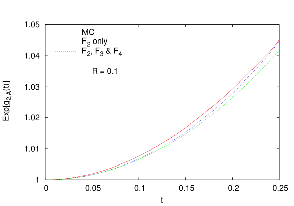
Figure 1: Comparisons of the analytical result to the output of the Monte Carlo program in the $k_{t}$ algorithm for two values of the jet radius.

The plots display the MC estimate of $\exp\left(g_{2,A}\right)$, the analytical result of the latter in the cases where (a) only the first coefficient $\mathcal{F}_{2}$ is included in the sum (29) and (b) the first three coefficients, $\mathcal{F}_{i=2,3,4}$, are included. The dependence of the clustering coefficients $\mathcal{F}_{i}$ on $R$, given in table 1, is taken into consideration.

One can clearly see that the function $\exp\left(g_{2,A}\right)$ is largely dominated by the first coefficient $\mathcal{F}_{2}$, with minor corrections from $\mathcal{F}_{3}$ and $\mathcal{F}_{4}$. For instance for $R=1.0$ the $\mathcal{F}_{2}$, $\mathcal{F}_{3}$ and $\mathcal{F}_{4}$ coefficients (put alone in turn) induce a correction to the anti-$k_{t}$ resummed distribution of 1.6%, 0.06%, 0.002% and 4.8%, 0.3% and 0.02% for $t=0.15$ and $0.25$ respectively. This can be understood from eq. (29): in addition to being smaller than $\mathcal{F}_{2}$, the higher-gluon coefficients $\mathcal{F}_{n}$ ($n\geq 3$) are suppressed by a factorial factor ($n!$), thus leading to a fast convergence. Given the agreement between our analytical estimate and the output of the Monte Carlo, and given that the function $\exp(g_{2,A})$ contributes at most $\mathcal{O}(5\%)$, we conclude that our results for the resummed clustering logs are phenomenologically accurate for jet radii up to order unity, and that missing higher-order coefficients $\mathcal{F}_{n}$ ($n\geq 5$) are unimportant.

Lastly, we plot in fig. 2, the MC results of the function $\exp(g_{2,A})$ for various jet radii. The plots unequivocally indicate that for a fixed $t$, say $0.15$, the function $g_{2,A}$ varies very slowly with $R$ for $R\leq 1$ and grows relatively rapidly as $R>1$. Such a behaviour may be explained by the analytical formula of $\mathcal{F}_{2}$, eq. (40), where the first correction to the small–$R$ result is proportional to $R^{4}$.

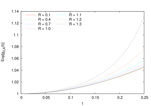
Figure 2: The output of the Monte Carlo program in the $k_{t}$ algorithm for various jet radii.

6.1 Non-global logs

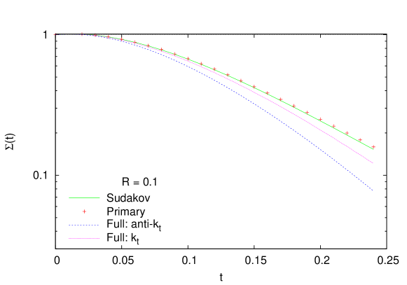
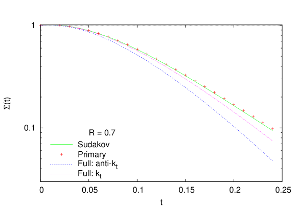
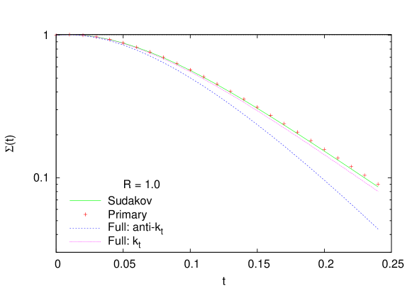
Figure 3: Comparisons of the Sudakov result, the correct primary result and the full result including non-global logarithms with and without clustering, as detailed in the main text.

As a final task, we plot in Fig. 3 the full resummed jet mass distribution in the $k_{t}$ algorithm, eq. (4), including the non-global factor $\mathcal{S}(t)$ in the large-$N_{c}$ limit, for various jet radii. In the figure, “Sudakov” refers to the Sudakov anti-$k_{t}$ form factor, $\Sigma^{\mathrm{anti-k_{t}}}$, “primary” refers to the primary form factor in the $k_{t}$ algorithm containing the clustering logarithms, $\Sigma^{k_{t}}$ (eq. (28)), “Full: anti-$k_{t}$” refers to the full anti-$k_{t}$ resummation, $\Sigma^{\mathrm{anti-k_{t}}}\,\mathcal{S}^{\mathrm{anti-k_{t}}}(t)$ and “Full: $k_{t}$” refers to $\Sigma^{k_{t}}\,\mathcal{S}^{k_{t}}(t)$. We notice that the inclusion of non-global logs leads to a noticeably large reduction of the full resummed result for the anti-$k_{t}$ algorithm case, while in the $k_{t}$ algorithm the reduction is moderate.

As is well known by now [21, 22, 23, 37], clustering reduces the impact of non-global logs through restricting the available phase-space for their contribution. This is also the case with the jet mass distribution where we note, for instance, that for $t=0.15$ the impact of non-global logs in the anti-$k_{t}$ algorithm (for $R=0.1,0.7$ and $1.0$) is a 24% reduction of the global part, while in the$k_{t}$ clustering case this is merely 7% (for $R=0.1$ and $R=0.7$) and 4% for $R=1.0$. We further notice that for small values of the jet radius, $\mathcal{S}(t)$ is independent of $R$. While this is true for all values of $R$ in the anti–$k_{t}$ algorithm , in the $k_{t}$ algorithm $\mathcal{S}$ falls down as $R$ becomes larger. This is evident in the $R=1.0$ plot in Fig. 3.

7 Conclusions

In this paper we have considered the possibility of exponentiation of clustering logs in the $k_{t}$ and C/A algorithms. We have found, by explicit calculations of the first few orders (up to $\mathcal{O}(\alpha_{s}^{4})$, and including, for the first time in literature, the full jet radius dependence), that the perturbative expansion of the invariant jet mass distribution exhibits a pattern of an expansion of an exponential. Consequently we were able to write an all-orders partially resummed expression for primary emission clustering logs. We further checked our formula against the output of a numerical Monte Carlo and found a good agreement, within the accuracy of our calculations. We have therefore concluded that missing higher-order single-log terms in our resummed distribution have a negligible impact on the total resummed distribution for typical values of jet radii (up to order unity).

Furthermore, we have briefly discussed the impact of the inclusion of non-global logs on the total resummed distribution. We confirmed previous observations concerning the facts that (a) non-global logs reduce the Sudakov peak of the distribution and that (b) such an impact is diminished when clustering is imposed on final-state particles.

We note that the calculations we performed here can readily be generalised to a large class of non-global observables defined using the $k_{t}$ or C/A algorithm, where the observable is sensitive to soft emissions in a restricted region of phase space, e.g. angularities [35]. Since the calculations of the coefficients $\mathcal{F}_{n}$ presented here are in fact independent of the jet shape and depend only on the angular configurations introduced by the clustering algorithm, then the effect of jet clustering can simply be included for any generic observable $v$ (being sensitive to soft and collinear emissions inside the jet only) by introducing the exponential function $\exp[g_{2,A}]$, with exactly the same coefficients $\mathcal{F}_{n}$ we computed here. The only difference is the argument of the logarithm essentially becoming $R^{2}/v$.

Although we have confined ourselves to studying the single jet mass distribution in $e^{+}e^{-}$ annihilation, the extension of our work to, e.g. monojet production at the LHC (such as $Z$+ jet, which is an important channel in looking at BSM physics, and for which a calculation in the anti-$k_{t}$ algorithm has recently been performed [39]) can readily be performed. In [38] we consider the extension of the work of ref. [39], which is carried out in the anti-$k_{t}$ jet algorithm, to the case where final-state jets are defined in the $k_{t}$ (and C/A) jet algorithms. We employ the techniques developed for $e^{+}e^{-}$ colliders in this paper to compute the full $R$-dependent resummed clustering logs as well as non-global logs for hadron colliders. Although the calculations for the latter are much more involved, no major deviations from the overall picture drawn at the current paper are anticipated.

Appendix A Full $R$-dependence of clustering coefficients

Here we present a calculation of the dependence of the coefficient of the clustering logs $\mathcal{F}_{2}$ away from the small-angles (thus small-$R$) approximation. To do so, it is easier to work with transverse momentum, (pseudo-)rapidity and azimuthal angle with respect to the beam axis, $(k_{t},\eta,\phi)$, variables instead of energy and polar angles, as performed in sec. 3. We also specialise to the threshold limit in which the trigged jet is created at $90^{\circ}$ to the beam (which is along the $z$-axis). Our calculations can straightforwardly be extended to the case where the triggered jet is at an arbitrary rapidity. We parametrise the outgoing four-momenta as:

$$p_{1} = \frac{Q}{2}(1,1,0,0),$$

$$p_{2} = \frac{Q}{2}(1,-1,0,0),$$

$$k_{i} = k_{ti}(\cosh\eta_{i},\cos\phi_{i},\sin\phi_{i},\sinh\eta_{i}),$$ (31)

with $i=1,2$ for the two gluons respectively. In terms of the new variables, the clustering function (eq. (5)) reads:

$$\Xi_{2}(k_{1},k_{2})=\Theta(d_{1j}-R^{2})\Theta(R^{2}-d_{2j})\Theta(d_{2j}-d_{12}),$$ (32)

with

$$d_{1j}=\eta_{1}^{2}+\phi_{1}^{2},\qquad d_{2j}=\eta_{2}^{2}+\phi_{2}^{2},\qquad d_{12}=(\eta_{1}-\eta_{2})^{2}+(\phi_{1}-\phi_{2})^{2}.$$ (33)

In this coordinate system the jet mass becomes:

$$\rho=\frac{2p_{1}.k_{i}}{Q^{2}/4}=\frac{4k_{ti}}{Q}(\cosh\eta_{i}-\cos\phi_{i})=2x_{i}\left(1-\frac{\cos\phi_{i}}{\cosh\eta_{i}}\right),$$ (34)

when particle $k_{i}$ is recombined with the triggered $p_{1}$ jet. In the above we expressed the jet mass in terms of the energy fraction $x_{i}=2\omega_{i}/Q$, with $\omega_{i}=k_{ti}\cosh\eta_{i}$.

The probability of a single virtual soft gluon correction is given by:

$$d\Gamma_{i}=-\frac{d^{3}\vec{k}_{i}}{2\omega_{i}(2\pi)^{3}}g_{s}^{2}C_{F}\frac{2(p_{1}.p_{2})}{(p_{1}.k_{i})(p_{2}.k_{i})}=-\frac{C_{F}\alpha_{s}}{\pi}\frac{dx_{i}}{x_{i}}d\eta\frac{d\phi_{i}}{\pi}\frac{1}{\cosh^{2}\eta_{i}-\cos^{2}\phi_{i}},$$ (35)

where we note here that the collinear limit to the triggered jet $p_{1}$ corresponds to $\eta_{i}\to 0$ and $\phi_{i}\to 0$.

Thus we can write the correction term due to clustering (eq. (6)) as:

$$\Sigma^{\rm{clus}}_{2}=\frac{1}{2!}\int\prod_{i}^{2}d\Gamma_{i}\Theta\left(x_{i}-\frac{\cosh\eta_{i}}{2(\cosh\eta_{i}-\cos\phi_{i})}\rho\right)\Xi_{2}(k_{1},k_{2}).$$ (36)

Performing the energy-fraction integration yields an expression identical to eq. (10) with the full $R$-dependent coefficient, $\mathcal{F}_{2}(R)$, given by:

$$\mathcal{F}_{2}(R)=\frac{1}{\pi^{2}}\int d\eta_{1}d\phi_{1}d\eta_{2}d\phi_{2}\frac{1}{\cosh^{2}\eta_{1}-\cos^{2}\phi_{1}}\frac{1}{\cosh^{2}\eta_{2}-\cos^{2}\phi_{2}}\Xi_{2}(k_{1},k_{2}).$$ (37)

This integration can be performed numerically to extract the value of $\mathcal{F}_{2}$ for arbitrary $R$. However it proves useful, in the simple case of $\mathcal{F}_{2}$ in order to obtain an analytic expression at least as a power-series, to introduce the polar variables $r$ and $\alpha$ defined by:

$$\eta=r\cos\alpha,\qquad\phi=r\sin\alpha.$$ (38)

We rewrite eq. (37) as:

$$\mathcal{F}_{2}=\frac{1}{\pi^{2}}\int_{R}^{\infty}r_{1}dr_{1}\int_{-\pi}^{\pi}d\alpha_{1}\int_{0}^{R}r_{2}dr_{2}\int_{-\pi}^{\pi}d\alpha_{2}\Theta(2r_{2}\cos(\alpha_{2}-\alpha_{1})-r_{1})\times\\ \times\frac{1}{\cosh^{2}(r_{1}\cos\alpha_{1})-\cos^{2}(r_{1}\sin\alpha_{1})}\,\,\frac{1}{\cosh^{2}(r_{2}\cos\alpha_{2})-\cos^{2}(r_{2}\sin\alpha_{2})}.$$ (39)

We note that one can expand the second line of eq. (39) in powers of $r_{i}$ so as to write the result as a power-series in $R$. To first order, the second line expands as $1/r_{1}^{2}1/r_{2}^{2}$. We thus immediately identify this integral as the one for the small-angles approximation, whose result is $\pi^{2}/54\approx 0.183$. Performing higher-order integrals of the expansion of the integrand yields the following result:

$$\mathcal{F}_{2}(R)=0.183+0.0246R^{4}+0.00183R^{8}+0.000135R^{12}+\mathcal{O}(R^{16}).$$ (40)

This expansion is actually valid for values of $R$ up to order unity, a claim which is backed-up by fully performing the integral (39) numerically via Monte Carlo methods and comparing to the analytical estimate (40), fig. 4. We note that the clustering coefficient varies very slowly with $R$.

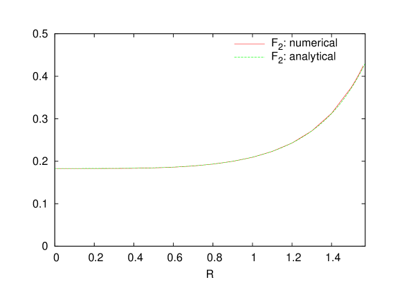
Figure 4: Full $R$-dependence of the two-gluon clustering coefficient $\mathcal{F}_{2}$.

Finally we note that the calculation of $\mathcal{F}_{3}^{(\mathrm{C/A})}$ and $\mathcal{F}_{4}$ may be performed in the same way. Schematically we have:

$$\mathcal{F}_{n}(R)=\frac{1}{\pi^{n}}\int\prod_{i}^{n}d\eta_{i}d\phi_{i}\frac{1}{\cosh^{2}\eta_{i}-\cos^{2}\phi_{i}}\Xi_{n}(k_{1},k_{2},\cdots,k_{n}),$$ (41)

where the step function $\Xi_{n}$ is expressed in terms of the distances $d_{i}=\eta_{i}^{2}+\phi_{i}^{2}$ and $d_{ij}=\delta\eta_{ij}^{2}+\delta\phi_{ij}^{2}$, respectively replacing $\theta_{i}$ and $\theta_{ij}$ in, e.g. eq. (LABEL:eq:ClustFun3kt). We provide full numerical estimates for all coefficients in table 1.

$R$	$0$	$0.1$	$0.4$	$0.7$	$1.0$	$1.2$
$\mathcal{F}_{2}$	$0.183$	$0.184$	$0.184$	$0.188$	$0.208$	$0.242$
$\mathcal{F}_{3}$	$-0.052$	$-0.053$	$-0.053$	$-0.055$	$-0.061$	$-0.072$
$\mathcal{F}_{3}^{\mathrm{C/A}}$	$-0.028$	$-0.029$	$-0.029$	$-0.029$	$-0.030$	$-0.031$
$\mathcal{F}_{4}$	$0.022$	$0.023$	$0.023$	$0.023$	$0.024$	$0.027$

Table 1: Estimates of the clustering coefficients $\mathcal{F}_{n}$ for $n=2,3,4$ at different values of the jet radius $R$ in the $k_{t}$ and C/A algorithms. Recall that $\mathcal{F}_{2}^{\mathrm{C/A}}=\mathcal{F}_{2}^{k_{t}}(\equiv\mathcal{F}_{2})$ and that $\mathcal{F}_{4}^{\mathrm{C/A}}$ has not been computed. Note that $\mathcal{F}_{3}^{\mathrm{C/A}}$ and $\mathcal{F}_{4}$ are more difficult to evaluate numerically than $\mathcal{F}_{3}$ (and obviously $\mathcal{F}_{2}$). Thus their final answers are subjected to larger errors.

References

- [1] M. Dasgupta and G. P. Salam, Event shapes in annihilation and deep inelastic scattering, J. Phys. G 30 (2004) R143 [hep-ph/0312283].
- [2] R. K. Ellis, W. J. Stirling and B. R. Webber, QCD and Collider Physics, Cambridge University Press, 1996.
- [3] S. Bethke, 2002, Nucl. Phys. 121 (Proc. Suppl.) (2003) 74 [hep-ex/0211012].
- [4] M. Beneke, Renormalons, Phys. Rept. 317 (1999) 1 [hep-ph/9807443].
- [5] G. Corcella, I. G. Knowles, G. Marchesini, S. Moretti, K. Odagiri, P. Richardson, M. H. Seymour and B. R. Webber, HERWIG 6: An Event generator for hadron emission reactions with interfering gluons (including supersymmetric processes), J. High Energy Phys. 01 (2001) 010 [hep-ph/0011363].
- [6] T. Sjostrand, S. Mrenna and P. Z. Skands, PYTHIA 6.4 Physics and Manual, J. High Energy Phys. 05 (2006) 026 [hep-ph/0603175].
- [7] A. Altheimer, S. Arora, L. Asquith, G. Brooijmans, J. Butterworth, M. Campanelli, B. Chapleau and A. E. Cholakian et al., Jet Substructure at the Tevatron and LHC: New results, new tools, new benchmarks, J. Phys. G 39 (2012) 063001 [\arXivid1201.0008 [hep-ph]].
- [8] J. M. Butterworth, A. R. Davison, M. Rubin and G. P. Salam, Jet substructure as a new Higgs search channel at the LHC, Phys. Rev. Lett. 100 (2008) 242001 [\arXivid0802.2470 [hep-ph]].
- [9] A. Abdesselam et al., Boosted objects: A Probe of beyond the Standard Model physics, Eur. Phys. J. C 71 (2011) 1661 [\arXivid1012.5412 [hep-ph]].
- [10] W. Skiba and D. Tucker-Smith, Using jet mass to discover vector quarks at the LHC, Phys. Rev. D 75 (2007) 115010 [hep-ph/0701247].
- [11] L. G. Almeida, S. J. Lee, G. Perez, G. F. Sterman, I. Sung and J. Virzi, Substructure of high- Jets at the LHC, Phys. Rev. D 79 (2009) 074017 [\arXivid0807.0234 [hep-ph]].
- [12] S. D. Ellis, C. K. Vermilion and J. R. Walsh, Techniques for improved heavy particle searches with jet substructure, Phys. Rev. D 80 (2009) 051501 [\arXivid0903.5081 [hep-ph]].
- [13] G. D. Kribs, A. Martin, T. S. Roy and M. Spannowsky, Discovering the Higgs Boson in New Physics Events using Jet Substructure, Phys. Rev. D 81 (2010) 111501 [\arXivid0912.4731 [hep-ph]].
- [14] S. Catani, L. Trentadue, G. Turnock and B. R. Webber, Resummation of large logs in event shape distributions, Nucl. Phys. B 407 (1993) 3.
- [15] A. Banfi, G. P. Salam and G. Zanderighi, Semi-numerical resummation of event shapes, J. High Energy Phys. 01 (2002) 018 [hep-ph/0112156].
- [16] A. Banfi, G. P. Salam and G. Zanderighi, Principles of general final-state resummation and automated implementation, J. High Energy Phys. 03 (2005) 073 [hep-ph/0407286].
- [17] A. Gehrmann-De Ridder, T. Gehrmann, E. W. N. Glover and G. Heinrich, NNLO corrections to event shapes in annihilation, J. High Energy Phys. 12 (2007) 094 [\arXivid0711.4711 [hep-ph]].
- [18] M. Dasgupta, L. Magnea and G. P. Salam, Non-perturbative QCD effects in jets at hadron colliders, J. High Energy Phys. 02 (2008) 055 [\arXivid0712.3014 [hep-ph]].
- [19] M. Dasgupta and G. P. Salam, Resummation of nonglobal QCD observables, Phys. Lett. B 512 (2001) 323 [hep-ph/0104277].
- [20] M. Dasgupta and G. P. Salam, Accounting for coherence in interjet flow: A Case study, J. High Energy Phys. 03 (2002) 017 [hep-ph/0203009].
- [21] R. B. Appleby and M. H. Seymour, Nonglobal logs in interjet energy flow with clustering requirement, J. High Energy Phys. 12 (2002) 063 [hep-ph/0211426].
- [22] Y. Delenda, R. Appleby, M. Dasgupta and A. Banfi, On QCD resummation with clustering, J. High Energy Phys. 12 (2006) 044 [hep-ph/0610242].
- [23] K. Khelifa-Kerfa, Non-global logs and clustering impact on jet mass with a jet veto distribution, J. High Energy Phys. 02 (2012) 072 [\arXivid1111.2016 [hep-ph]].
- [24] M. Cacciari, G. P. Salam and G. Soyez, The anti- jet clustering algorithm, J. High Energy Phys. 04 (2008) 063 [\arXivid0802.1189 [hep-ph]].
- [25] R. Kelley, J. R. Walsh and S. Zuberi, Abelian Non-Global Logs from Soft Gluon Clustering, [\arXivid1202.2361 [hep-ph]].
- [26] R. Kelley, J. R. Walsh and S. Zuberi, Disentangling Clustering Effects in Jet Algorithms, [\arXivid1203.2923 [hep-ph]].
- [27] A. Banfi and M. Dasgupta, Problems in resumming interjet energy flows with clustering, Phys. Lett. B 628 (2005) 49 [hep-ph/0508159].
- [28] A. Banfi, M. Dasgupta, K. Khelifa-Kerfa and S. Marzani, Non-global logs and jet algorithms in high- jet shapes, J. High Energy Phys. 08 (2010) 064 [\arXivid1004.3483 [hep-ph]].
- [29] Y. .L. Dokshitzer and G. Marchesini, On large angle multiple gluon radiation, J. High Energy Phys. 03 (2003) 040 [hep-ph/0303101].
- [30] S. Catani, Y. L. Dokshitzer, M. H. Seymour and B. R. Webber, Longitudinally invariant clustering algorithms for hadron hadron collisions, Nucl. Phys. B 406 (1993) 187; and refs. therein.
- [31] S. D. Ellis and D. E. Soper, Successive combination jet algorithm for hadron collisions, Phys. Rev. D 48 (1993) 3160 [hep-ph/9305266].
- [32] C. W. Bauer, S. Fleming and M. E. Luke, Summing Sudakov logarithms in in effective field theory, Phys. Rev. D 63 (2000) 014006 [hep-ph/0005275]; C. W. Bauer, S. Fleming, D. Pirjol and I. W. Stewart, An Effective field theory for collinear and soft gluons: Heavy to light decays, Phys. Rev. D 63 (2001) 114020 [hep-ph/0011336]; C. W. Bauer, D. Pirjol and I. W. Stewart, Soft collinear factorization in effective field theory, Phys. Rev. D 65 (2002) 054022 [hep-ph/0109045].
- [33] Y. L. Dokshitzer, G. D. Leder, S. Moretti and B. R. Webber, Better jet clustering algorithms, J. High Energy Phys. 08 (1997) 001 [hep-ph/9707323]; M. Wobisch and T. Wengler, Hadronization corrections to jet cross sections in deep-inelastic scattering, Proceedings of the Workshop on Monte Carlo Generators for HERA Physics, Hamburg, Germany, 27-30 April 1998 [hep-ph/9907280].
- [34] S. D. Ellis, A. Hornig, C. Lee, C. K. Vermilion and J. R. Walsh, Consistent Factorization of Jet Observables in Exclusive Multijet Cross-Sections, Phys. Lett. B 689 (2010) 82 [\arXivid0912.0262 [hep-ph]].
- [35] S. D. Ellis, C. K. Vermilion, J. R. Walsh, A. Hornig and C. Lee, Jet Shapes and Jet Algorithms in SCET, J. High Energy Phys. 11 (2010) 101 [\arXivid1001.0014 [hep-ph]].
- [36] M. Cacciari, G. P. Salam and G. Soyez, FastJet user manual, Eur. Phys. J. C 72 (2012) 1896 [\arXivid1111.6097 [hep-ph]].
- [37] Hornig, Andrew and Lee, Christopher and Walsh, Jonathan R. and Zuberi, Saba, Double Non-Global Logarithms In-N-Out of Jets, J. High Energy Phys. 01 (2012) 149, [hep-ph/1110.0004],
- [38] K. Khelifa–Kerfa and Y. Delenda, in preparation.
- [39] M. Dasgupta, K. Khelifa-Kerfa, S. Marzani and M. Spannowsky, On jet mass distributions in Z+jet and dijet processes at the LHC, [\arXivid1207.1640].