Nonmonotone Barzilai-Borwein Gradient Algorithm for $\ell_{1}$-Regularized Nonsmooth Minimization in Compressive Sensing

Abstract

This paper is devoted to minimizing the sum of a smooth function and a nonsmooth $\ell_{1}$-regularized term. This problem as a special cases includes the $\ell_{1}$-regularized convex minimization problem in signal processing, compressive sensing, machine learning, data mining, etc. However, the non-differentiability of the $\ell_{1}$-norm causes more challenging especially in large problems encountered in many practical applications. This paper proposes, analyzes, and tests a Barzilai-Borwein gradient algorithm. At each iteration, the generated search direction enjoys descent property and can be easily derived by minimizing a local approximal quadratic model and simultaneously taking the favorable structure of the $\ell_{1}$-norm. Moreover, a nonmonotone line search technique is incorporated to find a suitable stepsize along this direction. The algorithm is easily performed, where the values of the objective function and the gradient of the smooth term are required at per-iteration. Under some conditions, the proposed algorithm is shown to be globally convergent. The limited experiments by using some nonconvex unconstrained problems from CUTEr library with additive $\ell_{1}$-regularization illustrate that the proposed algorithm performs quite well. Extensive experiments for $\ell_{1}$-regularized least squares problems in compressive sensing verify that our algorithm compares favorably with several state-of-the-art algorithms which are specifically designed in recent years.

1 Introduction

The focus of this paper is on the following structured minimization

$$\min_{x\in\mathbb{R}^{n}}\ F(x)=f(x)+\mu\|x\|_{1},$$ (1)

where $f:\mathbb{R}^{n}\rightarrow\mathbb{R}$ is a continuously differentiable (may be nonconvex) function that is bounded below; $\|\cdot\|_{1}$ denotes the $\ell_{1}$-norm of a vector; parameter $\mu>0$ is used to trade off both terms for minimization. Due to its structure, problem (1) covers a wide range of apparently related formulations in different scientific fields including linear inverse problem, signal/image processing, compressive sensing, and machine learning.

1.1 Problem formulations

A popular special case of model (1) is the $\ell_{1}$-norm regularized least square problem

$$\min_{x\in\mathbb{R}^{n}}\frac{1}{2}\|Ax-b\|_{2}^{2}+\mu\|x\|_{1},$$ (2)

where $A\in\mathbb{R}^{m\times n}$ $(m\ll n)$ is a linear operator, and $b\in\mathbb{R}^{m}$ is an observation. Model (2) mainly appears in compressive sensing — an emerging methodology in digital signal processing, and has attracted intensive research activities over the past years [11, 12, 10, 13, 20]. Compressive sensing is based on the fact that if the original signal is sparse or approximately sparse in some orthogonal basis, an exact restoration can be produced via solving problem (2).

Another prevalent case of (1) that has been achieved much interest in machine learning is the linear and logistic regression. Given the training date $A=[a_{1},\cdots,a_{m}]^{\top}\in\mathbb{R}^{m\times n}$ and class labels $y\in\{-1,+1\}^{m}$. A linear classifier is a hyperplane $\{w_{i}:x^{\top}a_{i}+b=0\}$, where $x\in\mathbb{R}^{n}$ is a set of weights and $b\in\mathbb{R}$ is the intercept. A frequently used model is the $\ell_{2}$-loss support vector machine

$$\min_{x\in\mathbb{R}^{m},b\in\mathbb{R}}\sum_{i=1}^{m}\max\{0,1-y_{i}(x^{\top}a_{i}+b)\}^{2}+\mu\|x\|_{1},$$ (3)

Because of the ”max” operation, the $\ell_{2}$-loos function is continuous, but not differentiable. Based on the conditional probability, another popular model is the logistic regression

$$\min_{x\in\mathbb{R}^{n},b\in\mathbb{R}}\sum_{i=1}^{m}\text{log}\Big{(}1+e^{-(x^{\top}a_{i}+b)y_{i}}\Big{)}+\mu\|x\|_{1}.$$ (4)

Obviously, the logistic loss function is twice differentiable.

Although the models of these problems have similar structures, they may be very different from real-data point of view. For example, in compressive sensing, the length of measurement $m$ is much smaller than the length of original signal $(m\ll n)$ and the encoding matrix $A$ is dense. However, in machine learning, the numbers of instance $m$ and features $n$ are both large and the data $A$ is very sparse.

1.2 Existing algorithms

Since the $\ell_{1}$-regularized term is non-differentiable when $x$ contains values of zero, the use of the standard unconstrained smooth optimization tools are generally precluded. In the past decades, a wide variety of approaches has been proposed, analyzed, and implemented in compressive sensing and machine learning literatures. This includes a variety of algorithms for special cases where $f(x)$ has a specific functional form such as the least square (2), the square loss (3) and the logistic loss (4). In the following, we briefly review some of them in each literature.

The first popular approach falls into the coordinate descent method. At the current iterate $x_{k}$, the simple coordinate descent method updates one component at a time to generate $x_{k}^{j}$, $j=1,\ldots,n+1$, such that $x_{k}^{1}=x_{k}$, $x_{k}^{n+1}=x_{k+1}$, and solves a one-dimensional subproblem

$$\min_{z}\quad F(x_{k}^{j}+ze^{j})-F(x_{k}^{j}),$$ (5)

where $e^{j}$ is defined as the $j$-th column of an identity matrix. Clearly, the objective function has one variable, and one non-differentiable point at $z=-e^{j}$. To solve the logistic regression model (4), BBR [23] solves the sub-problem approximately by the use of trust region method with Newton step; CDN [14] improves BBR’s performance by applying a one-dimensional Newton method and a line search technique. Instead of cyclically updating one component at each time, the stochastic coordinate descent method [35] randomly selects the working components to attain better performance; the block coordinate gradient descent algorithm — CGD [38, 43] is based on the approximated convex quadratic model for $f$, and selects the working variables with some rules.

The second type of approach is to transform model (1) into an equivalent box-constrained optimization problem by variable splitting. Let $x=u-v$ with $u_{i}=\max\{0,x_{i}\}$ and $v_{i}=\max\{0,-x_{i}\}$. Then, model (1) can be reformulated equivalently as

$$\min_{u,v}f(u-v)+\mu\sum_{i=1}^{n}(u_{i}+v_{i}),\quad\text{s.t.}\ u\geq 0,\quad v\geq 0.$$ (6)

The objective function and constraints are smooth, and therefore, it can be solved by any standard box-constrained optimization technique. However, an obvious drawback of this approach is that it doubles the number of variables. GPSR [22] solves (6), and subsequently solves (2), by using Barzilai-Borwein gradient method [2] with an efficient nonmonotone line search [24]. It is actually an application of the well-known spectral projection gradient [8] in compressive sensing. Trust region Newton algorithm — TRON [28, 42] minimizes (6), then solves the logistic regression model (4), and exhibits powerful vitality by a series of comparisons. To solve (3) and (4), the interior-point algorithm [26, 27] forms a sequence of unconstrained approximations by appending a ‘barrier’ function to the objective function (6) which ensures that $u$ and $v$ remain sufficiently positive. Moreover, truncated Newton steps and preconditioned conjugate gradient iterations are used to produce the search direction.

The third type of method is to approximate the $\ell_{1}$-regularized term with a differentiable function. The simple approach replaces the $\ell_{1}$-norm with a sum of multi-quadric functions

$$l(x)\triangleq\sum_{i}^{n}\sqrt{x_{i}^{2}+\epsilon},$$

where $\epsilon$ is a small positive scalar. This function is twice-differentiable and $\lim_{\epsilon\rightarrow 0^{+}}l(x)=\|x\|_{1}$. Subsequently, several smooth unconstrained optimization approaches can be applied, based on this approximation. However, the performance of these algorithms is much influenced by the parameter values, and the condition number of the corresponding Hessian matrix becomes larger as $\epsilon$ decreases. The Nesterov’s smoothing technique [29] is to construct smooth functions to approximate any general convex nonsmooth function. Based on this technique, NESTA [4] solves problem (2) by using first-order gradient information.

The fourth type of approach falls into the subgradient-based Newton-type algorithm. The important attempt in this class is from Andrew and Gao [1], who extend the well-known limited memory BFGS method [31] to solve $\ell_{1}$-regularized logistic regression model (4), and propose an orthant-wise limited memory quasi-Newton method — OWL-QN. At each iteration, this method computes a search direction over an orthant containing the previous point. The subspace BFGS method — subBFGS [41] involves an inner iteration approach to find the descent quasi-Newton direction and a subgradient Wolfe-condtions to determine the stepsize which ensures that the objective functions are decreasing. This method enjoys global convergence and is capable of solving general nonsmooth convex minimization problems.

Finally, to solve model (2), besides GPSR and NESTA, there are other numerous specially designed solvers. By an operator splitting technique, Hale, Yin and Zhang derive the iterative shrinkage/thresholding fixed-point continuation algorithm (FPC) [25]. By combining the interior-point algorithm in [26], FPC is also extended to solve large-scale $\ell_{1}$-regularized logistic regression in [36]. TwIST [7] and FISTA [3] speed up the performance of IST and have virtually the same complexity but with better convergence properties. Another closely related method is the sparse reconstruction algorithm SpaRSA [39], which is to minimize non-smooth convex problem with separable structures. SPGL1 [5] solves the lasso model (2) by the spectral gradient projection method with an efficient Euclidean projection on $\ell_{1}$-norm ball. The alternating directions method — YALL1 [40], investigates $\ell_{1}$-norm problems from either the primal or the dual forms and solves $\ell_{1}$-regularized problems with different types.

All the reviewed algorithms differ in various aspects such as the convergence speed, ease of implementation, and practical applicability. Moreover, there is no enough evidence to verify that which algorithm outperforms the others under all scenarios.

1.3 Contributions and organization

Although much progress has been achieved in solving the problem (1), these algorithms mainly deal with the case where $f$ is a convex function even a least square. In this paper, unlike all the reviewed algorithms, we propose a Barzilai-Borwein gradient algorithm for solving $\ell_{1}$-regularized nonsmooth minimization problems. At each iteration, we approximate $f$ locally by a convex quadratic model, where the Hessian is replaced by the multiplies of a spectral coefficient with an identity matrix. The search direction is determined by minimizing the quadratic model and taking full use of the $\ell_{1}$-norm structure. We show that the generated direction is descent which guarantees that there exists a positive stepsize along the direction. In our algorithm, we adopt the nonmonotone line search of Grippo, Lampariello, and Lucidi [24], which allows the function values to increase occasionally in some iteration but decrease in the whole iterative process. The attractive property of the nonmonotone line search is that it saves much number of function evaluations which should be the main computational burden in large dataset. The method is easily performed, where only the value of objective function and the gradient of the smooth term are needed at each iteration. We show that each cluster of the iterates generated by this algorithm is a stationary point of $F$. In this paper, although we mainly consider the $\ell_{1}$-regularizer, the $\ell_{2}$-norm regularization problem and the matrix trace norm problems can also be readily included in our framework. Thus, this broaden the capability of the algorithm. We implement the algorithm to solve problem (1) where $f$ is a nonconvex smooth function from CUTEr library to show its efficiency. Moreover, we also run the algorithm to solve $\ell_{1}$-regularized least square, and do performance comparisons with the state-of-the-art algorithms NESTA, CGD, TwIST, FPC and GPSR. The comparisons results show that the proposed algorithm is effective, comparable, and promising.

We organize the rest of this paper as follows. In Section 2, we briefly recall some preliminary results in optimization literature to motivate our work, construct the search direction, and present the steps of our algorithm along with some remarks. In Section 3, we establish the global convergence theorem under some mild conditions. In Section 4, we show that how to extend the algorithm to solve $\ell_{2}$-norm and matrix trace norm minimization problems. In Section 5, we present experiments to show the efficiency of the algorithm in solving the $\ell_{1}$-regularized nonconvex problem and least square problem. Finally, we conclude our paper in Section 6.

2 Algorithm

2.1 Preliminary results

First, consider the minimization of the smooth function without the $\ell_{1}$-norm regularization

$$\min_{x\in\mathbb{R}}f(x).$$ (1)

The basic idea of Newton’s method for this problem is to iteratively use the quadratic approximation $q_{k}$ to the objective function $f(x)$ at the current iterate $x_{k}$ and to minimize the approximation $q_{k}$. Let $f:\mathbb{R}^{n}\rightarrow\mathbb{R}$ be twice continuously differentiable, and its Hessian $G_{k}=\nabla^{2}f(x_{k})$ be positive definite. Function $f$ at the current $x_{k}$ is modeled by the quadratic approximation $q_{k}$,

$$f(x_{k}+s)\approx q_{k}(s)=f(x_{k})+\nabla f(x_{k})^{\top}s+\frac{1}{2}s^{\top}G_{k}s,$$

where $s=x-x_{k}$. Minimizing $q_{k}(s)$ yields

$$x_{k+1}=x_{k}-G_{k}^{-1}\nabla f(x_{k}),$$

which is Newton’s formula and $s_{k}=x_{k+1}-x_{k}=-G_{k}^{-1}\nabla f(x_{k})$ is the so-called Newton’s direction.

For the positive definite quadratic function, Newton’s method can reach the minimizer with one iteration. However, when the starting point is far away from the solution, it is not sure that $G_{k}$ is positive definite and Newton’s direction $d_{k}$ is a descent direction. Let the quadratic model of $f$ at $x_{k+1}$ be

$$f(x)\approx f(x_{k+1})+\nabla f(x_{k+1})^{\top}(x-x_{k+1})+\frac{1}{2}(x-x_{k+1})^{\top}G_{k+1}(x-x_{k+1}).$$

Finding the derivative yields

$$\nabla f(x)\approx\nabla f(x_{k+1})+G_{k+1}(x-x_{k+1}).$$

Setting $x=x_{k}$, $s_{k}=x_{k+1}-x_{k}$, and $y_{k}=\nabla f(x_{k+1})-\nabla f(x_{k})$ we get

$$G_{k+1}s_{k}\approx y_{k}.$$ (2)

For various practical problems, the computing efforts of the Hessian matrices are very expensive, or the evaluation of the Hessian is difficult; even the Hessian is not available analytically. These lead to the quasi-Newton method which generates a series of Hessian approximations by the use of the gradient, and at the same time maintains a fast rate of convergence. Instead of computing the Hessian $G_{k}$, quasi-Newton method constructs the Hessian approximation $B_{k}$, where the sequence $\{B_{k}\}$ possesses positive definiteness and satisfies

$$B_{k+1}s_{k}=y_{k}.$$ (3)

In general, such $B_{k+1}$ will be produced by updating $B_{k}$ with some typical and popular formulae such as BFGS, DFP, and SR1.

Unfortunately, the standard quasi-Newton algorithm, or even its limited memory versions, doesn’t scale well enough to train very large-scale models involving millions of variables and training instances, which are commonly encountered, for example, in natural language processing. The main computational burden of Newton-type algorithm is the storage of a large matrix at per-iteration, which may be out of the memory capability for a PC. It should be develop a matrix-free algorithm to deal with large-scale problems but also belongs to the quasi-Newton framework. For this purpose, it would like to furthermore simplify the approximation Hessian $B_{k}$ as a diagonal matrix with positive components, i.e., $B_{k}=\lambda_{k}I$ with an identity matrix $I$ and $\lambda_{k}>0$. Then, the quasi-Newton condition changes to the form

$$\lambda_{k+1}Is_{k}=y_{k}.$$

Multiplying both sides by $s_{k}^{\top}$, gives

$$\lambda_{k+1}^{(1)}=\frac{s_{k}^{\top}y_{k}}{\|s_{k}\|_{2}^{2}}.$$ (4)

Similarly, multiplying both sides by $y_{k}^{\top}$, yields

$$\lambda_{k+1}^{(2)}=\frac{\|y_{k}\|_{2}^{2}}{s_{k}^{\top}y_{k}}.$$ (5)

Observing both formulae, it indicates that if $s_{k}^{\top}y_{k}>0$, the matrix $\lambda_{k+1}I$ is positive definite, which ensures that the search direction $-\lambda_{k}^{-1}\nabla f(x_{k})$ is descent at current point.

The formulae (4) and (5) were firstly developed by Barzilai and Borwein [2] for the quadratic case of $f$. This method essentially consists the steepest descent method, and adopts the choice of (4) or (4) as the stepsize along a negative gradient direction. Barzilai and Borwein [2] showed that the corresponding iterative algorithm is R-superlinearly convergent for the quadratic case. Raydan [33] presented a globalization strategy based on nonmonotone line search [24] for the general non-quadratic case. Other developments in Barzilai and Borwein gradient algorithm can be found in [6, 15, 17, 18, 19, 32, 44].

2.2 Algorithm

Due to its simplicity and numerical efficiency, the Barzilai-Borwein gradient method is very effective to deal with large-scale smooth unconstrained minimization problems. However, the application of the Barilai-Borwein gradient algorithm to $\ell_{1}$-regularized nonsmooth optimization is problematic since the regularization is non-differentiable. In this subsection, we construct an iterative algorithm to solve the $\ell_{1}$-regularized structured nonconvex optimization problem. The algorithm can be described as the iterative form

$$x_{k+1}=x_{k}+\alpha_{k}d_{k},$$

where $\alpha_{k}$ is a stepsize, and $d_{k}$ is a search direction defined by minimizing a quadratic approximated model of $F$.

Now, we turn to our attention to consider the original problem with $\ell_{1}$-regularizer. Since $\ell_{1}$-term is not differentiable, hence, at current $x_{k}$, objective function $F$ is approximated by the quadratic approximation $Q_{k}$,

$$F(x_{k}+d)= f(x_{k}+d)+\mu\|x_{k}+d\|_{1}$$

$$\approx f(x_{k})+\nabla f(x_{k})^{\top}d+\frac{\lambda_{k}}{2}\|d\|_{2}^{2}+\mu\Big{[}\|x_{k}\|_{1}+\frac{\|x_{k}+hd\|_{1}-\|x_{k}\|_{1}}{h}\Big{]}\triangleq Q_{k}(d),$$ (6)

where $h$ is a small positive number. The term in $[\cdot]$ can be considered as an approximate Taylor expansion of $\|x_{k}+d\|_{1}$ with a small $h$, and the case $h=1$ reduces the equivalent form $\|x_{k}+d\|_{1}$. Minimizing (2.2) yields

$$\min_{d\in\mathbb{R}^{n}}Q_{k}(d)$$

$$\Leftrightarrow \min_{d\in\mathbb{R}^{n}}\nabla f(x_{k})^{\top}d+\frac{\lambda_{k}}{2}\|d\|_{2}^{2}+\frac{\mu}{h}\|x_{k}+hd\|_{1}$$

$$\Leftrightarrow \min_{d\in\mathbb{R}^{n}}\frac{h^{2}}{\lambda_{k}}\Big{(}\nabla f(x_{k})^{\top}d+\frac{\lambda_{k}}{2}\|d\|_{2}^{2}+\frac{\mu}{h}\|x_{k}+hd\|_{1}\Big{)}$$

$$\Leftrightarrow \min_{d\in\mathbb{R}^{n}}\frac{1}{2}\Big{\|}x_{k}+hd-\big{(}x_{k}-\frac{h}{\lambda_{k}}\nabla f(x_{k})\big{)}\Big{\|}_{2}^{2}+\frac{\mu h}{\lambda_{k}}\|x_{k}+hd\|_{1}$$

$$\Leftrightarrow \min_{d\in\mathbb{R}^{n}}\sum_{i=1}^{n}\Big{\{}\frac{1}{2}\Big{(}x_{k}^{i}+hd^{i}-\big{(}x_{k}^{i}-\frac{h}{\lambda_{k}}\nabla f^{i}(x_{k})\big{)}\Big{)}^{2}+\frac{\mu h}{\lambda_{k}}|x_{k}^{i}+hd^{i}|\Big{\}}$$ (7)

where $x_{k}^{i}$, $d^{i}$, and $\nabla f^{i}(x_{k})$ denote the $i$-th component of $x_{k}$, $d$, and $\nabla f(x_{k})$ respectively. The favorable structure of (7) admits the explicit solution

$$x_{k}^{i}+hd_{k}^{i}=\max\Big{\{}\Big{|}x_{k}^{i}-\frac{h}{\lambda_{k}}\nabla f^{i}(x_{k}^{i})\Big{|}-\frac{\mu h}{\lambda_{k}},0\Big{\}}\frac{x_{k}^{i}-\frac{h}{\lambda_{k}}\nabla f^{i}(x_{k})}{|x_{k}^{i}-\frac{h}{\lambda_{k}}\nabla f^{i}(x_{k})|}.$$

Hence, the search direction at current point is

$$d_{k}=-\frac{1}{h}\Big{[}x_{k}-\max\Big{\{}\Big{|}x_{k}-\frac{h}{\lambda_{k}}\nabla f(x_{k})\Big{|}-\frac{\mu h}{\lambda_{k}},0\Big{\}}\frac{x_{k}-\frac{h}{\lambda_{k}}\nabla f(x_{k})}{|x_{k}-\frac{h}{\lambda_{k}}\nabla f(x_{k})|}\Big{]}.$$ (8)

where $|\cdot|$ and $``\max"$ are interpreted as componentwise and the convention $0\cdot 0/0=0$ is followed. When $\mu=0$, (8) reduces to $d_{k}=-\lambda_{k}^{-1}\nabla f(x_{k})$, i.e., the traditional Barizilai-Borwein gradient algorithm in smooth optimization. The key motivation for this formulation is that the optimization problem in Eq. (7) can be easily solved by exploiting the structure of the $\ell_{1}$-norm.

Lemma 1.

For any real vectors $a\in\mathbb{R}^{n}$ and $b\in\mathbb{R}^{n}$, the following function $L(x)$ is non-decreasing

$$L(x)=\frac{\|a+bx\|_{1}-\|a\|_{1}}{x},\quad x\in(0,\infty).$$ (9)

Proof.

Note that

$$L(x)=\frac{\|a+bx\|_{1}-\|a\|_{1}}{x}=\sum_{i}^{n}\frac{|a^{i}+b^{i}x|-|a^{i}|}{x}\triangleq\sum_{i}^{n}l^{i}(x),$$

hence, it reduces to prove that $l^{i}(x)$ is non-decreasing for each $i$.
(a). When $a^{i}\geq 0$ and $a^{i}x+b^{i}\geq 0$. It is clear that $l^{i}(x)=b^{i}$.
(b). When $a^{i}\geq 0$ and $a^{i}x+b^{i}\leq 0$, we have

$$l^{i}(x)=\frac{-2a^{i}-b^{i}x}{x}=\frac{-2a^{i}}{x}-b^{i}.$$

(c). When $a^{i}\leq 0$ and $a^{i}x+b^{i}\geq 0$, we have

$$l^{i}(x)=\frac{2a^{i}+b^{i}x}{x}=\frac{2a^{i}}{x}+b^{i}.$$

(d). When $a^{i}\leq 0$ and $a^{i}x+b^{i}\geq 0$, we have $l^{i}(x)=-b^{i}$.
It is not difficult to see that $l^{i}(x)$ is non-decreasing at each case. Hence, $L(x)$ is non-decreasing. ∎

The following lemma shows that the direction defined by (8) is descent if $d_{k}\neq 0$.

Lemma 2.

Suppose that $\lambda_{k}>0$ and $d_{k}$ is determined by (8). Then

$$F(x_{k}+\theta d_{k})\leq F(x_{k})+\theta\Big{[}\nabla f(x_{k})^{\top}d_{k}+\frac{\mu\|x_{k}+hd_{k}\|_{1}-\mu\|x_{k}\|_{1}}{h}\Big{]}+o(\theta)\quad\theta\in(0,h],$$ (10)

and

$$\nabla f(x_{k})^{\top}d_{k}+\frac{\mu\|x_{k}+hd_{k}\|_{1}-\mu\|x_{k}\|_{1}}{h}\leq-\frac{\lambda_{k}}{2}\|d_{k}\|_{2}^{2}.$$ (11)

Proof.

By the differentiability of $f$ and the convexity of $\|x\|_{1}$, we have that for any $\theta\in(0,h]$ ($\theta/h\in(0,1]$),

$$F(x_{k}+\theta d_{k})-F(x_{k}) =f(x_{k}+\theta d_{k})-f(x_{k})+\mu\|x_{k}+\theta d_{k}\|_{1}-\mu\|x_{k}\|_{1}$$

$$=f(x_{k}+\theta d_{k})-f(x_{k})+\mu\Big{\|}\frac{\theta}{h}(x_{k}+hd_{k})+(1-\frac{\theta}{h})x_{k}\Big{\|}_{1}-\mu\|x_{k}\|_{1}$$

$$\leq f(x_{k}+\theta d_{k})-f(x_{k})+\frac{\theta\mu}{h}\|x_{k}+hd_{k}\|_{1}+(1-\frac{\theta}{h})\mu\|x_{k}\|_{1}-\mu\|x_{k}\|_{1}$$

$$=\theta\nabla f(x_{k})^{\top}d_{k}+o(\theta)+\theta\Big{[}\frac{\mu}{h}\|x_{k}+hd_{k}\|_{1}-\frac{\mu}{h}\|x_{k}\|_{1}\Big{]},$$

which is exactly (10).

Noting that $d_{k}$ is the minimizer of (2.2) and $\theta\in(0,h]$, from (2.2) and the convexity of $\|x\|_{1}$, we have

$$\nabla f(x_{k})^{\top}d_{k}+\frac{\lambda_{k}}{2}\|d_{k}\|_{2}^{2}+\frac{\mu\|x_{k}+hd_{k}\|_{1}-\mu\|x_{k}\|_{1}}{h}$$

$$\leq \theta\nabla f(x_{k})^{\top}d_{k}+\frac{\lambda_{k}}{2}\|\theta d_{k}\|_{2}^{2}+\frac{\mu}{h}\|x_{k}+\theta hd_{k}\|_{1}-\frac{\mu}{h}\|x_{k}\|_{1}$$

$$\leq \theta\nabla f(x_{k})^{\top}d_{k}+\frac{\lambda_{k}\theta^{2}}{2}\|d_{k}\|_{2}^{2}+\frac{\theta\mu}{h^{2}}\|x_{k}+h^{2}d_{k}\|_{1}+\frac{\mu}{h}(1-\frac{\theta}{h})\|x_{k}\|_{1}-\frac{\mu}{h}\|x_{k}\|_{1}.$$

Hence,

$$(1-\theta)\nabla f(x_{k})^{\top}d_{k}+\frac{\mu}{h}\|x_{k}+hd_{k}\|_{1}-\frac{\theta\mu}{h^{2}}\|x_{k}+h^{2}d_{k}\|_{1}-\frac{\mu}{h}(1-\frac{\theta}{h})\|x_{k}\|_{1}\leq-\frac{\lambda_{k}}{2}(1-\theta^{2})\|d_{k}\|_{2}^{2}.$$ (12)

The last three terms of the left side in (12) can be re-organized as

$$\frac{\mu}{h}\Big{\{}\|x_{k}+hd_{k}\|_{1}-\frac{\theta}{h}\|x_{k}+h^{2}d_{k}\|_{1}-(1-\frac{\theta}{h})\|x_{k}\|_{1}\Big{\}}$$

$$= \frac{\mu}{h}\Big{\{}\|x_{k}+hd_{k}\|_{1}-\|x_{k}\|_{1}-\theta\Big{[}\frac{\|x_{k}+h^{2}d_{k}\|_{1}-\|x_{k}\|_{1}}{h}\Big{]}\Big{\}}$$

$$= \frac{\mu}{h}\Big{\{}\|x_{k}+hd_{k}\|_{1}-\|x_{k}\|_{1}-\theta\Big{[}h\cdot\frac{\|x_{k}+h^{2}d_{k}\|_{1}-\|x_{k}\|_{1}}{h^{2}}\Big{]}\Big{\}}$$

$$\geq \frac{\mu}{h}\Big{\{}\|x_{k}+hd_{k}\|_{1}-\|x_{k}\|_{1}-\theta\Big{[}h\cdot\frac{\|x_{k}+hd_{k}\|_{1}-\|x_{k}\|_{1}}{h}\Big{]}\Big{\}}$$

$$= \frac{\mu}{h}(1-\theta)\{\|x_{k}+hd_{k}\|_{1}-\|x_{k}\|_{1}\},$$ (13)

where the inequality is from Lemma 1. Combining (12) with (13), it produces

$$(1-\theta)\nabla f(x_{k})^{\top}d_{k}+(1-\theta)\frac{\mu\|x_{k}+hd_{k}\|_{1}-\mu\|x_{k}\|_{1}}{h}\leq-\frac{\lambda_{k}}{2}(1-\theta^{2})\|d_{k}\|_{2}^{2}.$$ (14)

Dividing both sides of (14) by $(1-\theta)$ and noting $\theta\in(0,h]$, we get the desirable result (11). ∎

When the search direction is determined, a suitable stepsize along this direction should be found to determine the next iterative point. In this paper, unlike the traditional Armijo line search or the Wolfe-Powell line search, we pay particular attention to a nonmonotone line search strategy. The traditional Armijo line search requires the function value to decrease monotonically at each iteration. As a result, it may cause the sequence of iterations following the bottom of a curved narrow valley, which commonly occurs in difficult nonlinear problems. To overcome this difficultly, a credible alternative is to allow an occasional increase in the objective function at each iteration. To easy comprehension of the proposed algorithm, we briefly recall the earliest nonmonotone line search technique by Grippo, Lampariello, and Lucidi [24]. Let $\delta_{k}\in(0,1)$, $\rho\in(0,1)$ and $\tilde{m}$ be a positive integer. The nonmonotone line search is to choose the smallest nonnegative integer $j_{k}$ such as the stepsize $\alpha_{k}=\tilde{\alpha}\rho^{j_{k}}$ satisfing

$$f(x_{k}+\alpha_{k}d_{k})\leq\max_{0\leq j\leq m(k)}f(x_{k-j})+\delta\alpha_{k}\nabla f(x_{k})^{\top}d_{k},$$ (15)

where

$$m(0)=0\quad\text{and}\quad 0\leq m(k)\leq\min\{m(k-1)+1,\tilde{m}\}.$$

If $m(k)=0$, the above nonmonotone line search reduces to the standard Armijo line search.

For the $\ell_{1}$-regularized nonsmooth problem (1), based on Lemma 2, the inequality (15) should be modified as

$$F(x_{k}+\alpha_{k}d_{k})\leq\max_{0\leq j\leq m(k)}F(x_{k-j})+\delta\alpha_{k}\Delta_{k},$$ (16)

where

$$\Delta_{k}=\nabla f(x_{k})^{\top}d_{k}+\frac{\mu\|x_{k}+hd_{k}\|_{1}-\mu\|x_{k}\|_{1}}{h}.$$ (17)

From (11), it clear that $\Delta_{k}\leq-\frac{\lambda_{k}}{2}\|d_{k}\|^{2}_{2}<0$ whenever $d_{k}\neq 0$. Hence, this shows that $\alpha_{k}$ given by (16) is well-defined.

In light of all derivations above, we now describe the nonmonotone Barzilai-Borwein gradient algorithm (abbreviated as NBBL1) as follows.

 

Algorithm 1.

(NBBL1)  Initialization: Choose $x_{0}$ and constants $\mu>0$. Constants $\tilde{\alpha}>0$, $\rho\in(0,1)$, $\delta\in(0,1)$, $h\in(0,1]$ and positive integer $\tilde{m}$. Set $k=0$.
Step 1. Stop if $\|d_{k}\|_{2}=0$. Otherwise, continue.
Step 2. Compute $d_{k}$ via (8).
Step 3. Compute $\alpha_{k}$ via (16).
Step 4. Let $x_{k+1}=x_{k}+\alpha_{k}d_{k}$.
Step 5. Let $k=k+1$. Go to Step 1.

   

Remark 1.

We have shown that if $\lambda_{k}>0$, then the generated direction is descent. However, in this case, the condition $\lambda_{k}>0$ may fail to be fulfilled and the hereditary descent property is not guaranteed any more. To cope with this defect, we should keep the sequence $\{\lambda_{k}\}$ uniformly bounded; that is, for sufficiently small $\lambda_{(\min)}>0$ and sufficiently large $\lambda_{(\max)}>0$, the $\lambda_{k}$ is forced as

$$\lambda_{k}=\min\{\lambda_{(\max)},\max\{\lambda_{k},\lambda_{(\min)}\}\}.$$

This approach ensures that $\lambda_{k}$ is bounded from zero and subsequently ensures that $d_{k}$ is descent at per-iteration.

Remark 2.

From Lemma 2, it is clear that there exists a constant $\theta\in(0,h]$ such that $x_{k}+\theta d_{k}$ is a descent point in sense of (10). Hence, in practical computation, it is suggested to choose the initial stepsize as $\tilde{\alpha}=h$.

3 Convergence analysis

This section is devoted to presenting some favorable properties of the generated direction and establishing the global convergence of Algorithm 1 subsequently. Our convergence result utilizes the following assumptions.

Assumption 1.

The level set $\Omega=\{x:f(x)\leq f(x_{0})\}$ is bounded.

Lemma 3.

Suppose that $\lambda_{k}>0$ and $d_{k}$ is defined by (8) with $h\in(0,1]$. Then $x_{k}$ is a stationary point of problem (1) if and only if $d_{k}=0$.

Proof.

If $d_{k}\neq 0$, then Lemma 2 shows that $d_{k}$ is descent direction at $x_{k}$, which implies that $x_{k}$ is not a stationary point of $F$. On the other hand, if $d_{k}=0$ is the solution of (7), for any $\alpha d\in\mathbb{R}^{n}$ with $\alpha>0$ we have

$$\alpha\nabla f(x_{k})^{\top}d+\frac{\lambda_{k}\alpha^{2}}{2}\|d\|_{2}^{2}+\frac{\mu}{h}\|x_{k}+\alpha hd\|_{1}\geq\frac{\mu}{h}\|x_{k}\|_{1}.$$ (1)

Since $f(x_{k}+\alpha d)-f(x_{k})=\alpha\nabla f(x_{k})^{\top}d+o(\alpha)$, this together with (1) yields

$$F^{\prime}(x_{k};d)= \lim_{\alpha\downarrow 0}\frac{f(x_{k}+\alpha d)-f(x_{k})+\mu\|x_{k}+\alpha d\|_{1}-\mu\|x_{k}\|_{1}}{\alpha}$$

$$= \lim_{\alpha\downarrow 0}\frac{\alpha\nabla f(x_{k})^{\top}d+o(\alpha)+\mu\|x_{k}+\alpha d\|_{1}-\mu\|x_{k}\|_{1}}{\alpha}$$

$$\geq \lim_{\alpha\downarrow 0}\Big{(}\frac{-\frac{\lambda_{k}\alpha^{2}}{2}\|d\|_{2}^{2}+o(\alpha)}{\alpha}+\frac{\big{[}\mu\|x_{k}+\alpha d\|_{1}-\mu\|x_{k}\|_{1}\big{]}-\big{[}\frac{\mu}{h}\|x_{k}+\alpha hd\|_{1}-\frac{\mu}{h}\|x_{k}\|_{1}\big{]}}{\alpha}\Big{)}.$$

$$\geq \lim_{\alpha\downarrow 0}\frac{-\frac{\lambda_{k}\alpha^{2}}{2}\|d\|_{2}^{2}+o(\alpha)}{\alpha}$$

$$= 0,$$

where the second inequality is from Lemma 1. Hence, $x_{k}$ is a stationary point of $F$. ∎

The proof of the following lemma is similar with the Theorem in [24].

Lemma 4.

Let $l(k)$ be an integer such that

$$k-m(k)\leq l(k)\leq k\quad\text{and}\quad F(x_{l(k)})=\max_{0\leq j\leq m(k)}F(x_{k-j}).$$

Then the sequence $\{F(x_{l(k)})\}$ is nonincreasing and the search direction $d_{l(k)}$ satisfies

$$\lim_{k\rightarrow\infty}\alpha_{l(k)}\|d_{l(k)}\|_{2}=0.$$ (2)

Proof.

From the definition of $m(k)$, we have $m(k+1)\leq m(k)+1$. Hence

$$F(x_{l(k+1)})= \max_{0\leq j\leq m(k+1)}F(x_{k+1-j})$$

$$\leq \max_{0\leq j\leq m(k)+1}F(x_{k+1-j})$$

$$= \max\{F(x_{l(k)}),F(x_{k+1})\}$$

$$= F(x_{l(k)}).$$

Moreover, by (16), we have for all $k>\tilde{m}$,

$$F(x_{l(k)}) =F(x_{l(k)-1}+\alpha_{l(k)-1}d_{l(k)-1})$$

$$\leq\max_{0\leq j\leq m(l(k)-1)}F(x_{l(k)-1-j})+\delta\alpha_{l(k)-1}\Delta_{l(k)-1}$$

$$=F(x_{l(l(k)-1)})+\delta\alpha_{l(k)-1}\Delta_{l(k)-1}.$$

By assumption 1, the sequence $\{F(x_{l(k)})\}$ admits a limit for $k\rightarrow\infty$. Hence, it follows that

$$\lim_{k\rightarrow\infty}\alpha_{l(k)}\Delta_{l(k)}=0.$$ (3)

On the other hand, from the definition of $\Delta_{k}$ in (17) and the inequality (11), it is not difficult to deduce that

$$\Delta_{l(k)}\leq-\frac{\lambda_{(\min)}}{2}\|d_{l(k)}\|_{2}^{2}<0.$$

Combining (3), yields

$$\lim_{k\rightarrow\infty}\alpha_{l(k)}\|d_{l(k)}\|_{2}^{2}=0,$$

which shows the desirable result (2). ∎

Theorem 5.

Let the sequence $\{x_{k}\}$ and $\{d_{k}\}$ generated by Algorithm 1. Then, there exists a subsequence $\mathcal{K}$ such that

$$\lim_{k\rightarrow\infty,k\in\mathcal{K}}\|d_{k}\|_{2}=0.$$ (4)

Proof.

From [24], it is clear that (2) also implies

$$\lim_{k\rightarrow\infty}\alpha_{k}\|d_{k}\|_{2}=0.$$ (5)

Now, let $\bar{x}$ be a limit point of $\{x_{k}\}$, and $\{x_{k}\}_{\mathcal{K}_{1}}$ be a subsequence of $\{x_{k}\}$ converging to $\bar{x}$. Then by (5) either $\lim\limits_{k\rightarrow\infty,k\in\mathcal{K}_{1}}\|d_{k}\|_{2}=0$, which implies $\|\bar{d}\|_{2}=0$, or there exists a subsequence $\{x_{k}\}_{\mathcal{K}}$ ($\mathcal{K}\subset\mathcal{K}_{1}$) such that

$$\lim_{k\rightarrow\infty,k\in\mathcal{K}}d_{k}\neq 0\quad\text{and}\quad\lim_{k\rightarrow\infty,k\in\mathcal{K}}\alpha_{k}=0.$$ (6)

In this case, we assume that there exists a constant $\epsilon>0$ such that

$$\|d_{k}\|_{2}\geq\epsilon,\quad\forall\ k\in\mathcal{K}.$$ (7)

Since $\alpha_{k}$ is the first value for satisfying (16), it follows from Step 3 in Algorithm 1 that there exists an index $\bar{k}$ such that, for all $k\geq\bar{k}$ and $k\in\mathcal{K}$,

$$F(x_{k}+\frac{\alpha_{k}}{\rho}d_{k})>\max_{0\leq j\leq m(k)}F(x_{k-j})+\delta\frac{\alpha_{k}}{\rho}\Delta_{k}\geq F(x_{k})+\delta\frac{\alpha_{k}}{\rho}\Delta_{k}.$$ (8)

Since $f$ is continuous differentiable, by the mean-value theorem on $f$, we can find there exists a constant $\theta_{k}\in(0,1)$, such that

$$f(x_{k}+\frac{\alpha_{k}}{\rho}d_{k})-f(x_{k})=\frac{\alpha_{k}}{\rho}\nabla f(x_{k}+\theta_{k}\frac{\alpha_{k}}{\rho}d_{k})^{\top}d_{k}.$$

By combining with (8), we have

$$\nabla f(x_{k}+\theta_{k}\frac{\alpha_{k}}{\rho}d_{k})^{\top}d_{k}+\frac{\mu\|x_{k}+\frac{\alpha_{k}}{\rho}d_{k}\|_{1}-\mu\|x_{k}\|_{1}}{\alpha_{k}/\rho}>\delta\Delta_{k}.$$ (9)

Since $\tilde{\alpha}=h$ and $\alpha_{k}\rightarrow 0$ in (6), we have $\alpha_{k}<\rho h$ as $k\rightarrow\infty$. It follows from Lemma 1 that

$$\frac{\mu\|x_{k}+\frac{\alpha_{k}}{\rho}d_{k}\|_{1}-\mu\|x_{k}\|_{1}}{\alpha_{k}/\rho}-\frac{\mu\|x_{k}+hd_{k}\|_{1}-\mu\|x_{k}\|_{1}}{h}\leq 0.$$

Subtracting both sides of (9) by $\Delta_{k}$ and noting the definition of $\Delta_{k}$, it is clear that

$$\nabla f(x_{k}+\theta_{k}\frac{\alpha_{k}}{\rho}d_{k})^{\top}d_{k}-\nabla f(x_{k})^{\top}d_{k}$$

$$\geq \nabla f(x_{k}+\theta_{k}\frac{\alpha_{k}}{\rho}d_{k})^{\top}d_{k}-\nabla f(x_{k})^{\top}d_{k}+\Big{[}\frac{\mu\|x_{k}+\frac{\alpha_{k}}{\rho}d_{k}\|_{1}-\mu\|x_{k}\|_{1}}{\alpha_{k}/\rho}-\frac{\mu\|x_{k}+hd_{k}\|_{1}-\mu\|x_{k}\|_{1}}{h}\Big{]}$$

$$> -(1-\delta)\Delta_{k}$$

$$\geq (1-\delta)\frac{\lambda_{(\min)}}{2}\|d_{k}\|_{2}^{2}.$$ (10)

Taking the limit as $k\in\mathcal{K}$, $k\rightarrow\infty$ in the both sides of (10) and using the smoothness of $f$, we obtain

$$0=\nabla f(\bar{x})^{\top}\bar{d}-\nabla f(\bar{x})^{\top}\bar{d}\geq(1-\delta)\frac{\lambda_{(\min)}}{2}\|\bar{d}\|_{2}^{2},$$

which implies $\|d_{k}\|_{2}\rightarrow 0$ as $k\in\mathcal{K}$, $k\rightarrow\infty$. This yields a contradiction because (7) indicates that $\|d_{k}\|_{2}$ is bounded. ∎

4 Some extensions

In this section, we show that our algorithm can be readily extended to solve $\ell_{2}$-norm and matrix trace norm minimization problems in machine learning; thus, broaden the applicable range of our approach significantly.

Firstly, we consider the $\ell_{2}$-regularization problem

$$\min_{x\in\mathbb{R}^{n}}\ F(x)=f(x)+\mu\|x\|_{2}.$$

It is not difficult to deduce that, the search direction $d_{k}$ is determined by minimizing

$$\min_{d\in\mathbb{R}^{n}}\frac{1}{2}\Big{\|}x_{k}+hd-\big{(}x_{k}-\frac{h}{\lambda_{k}}\nabla f(x_{k})\big{)}\Big{\|}_{2}^{2}+\frac{\mu h}{\lambda_{k}}\|x_{k}+hd\|_{2}.$$

From [21], the explicit solution is

$$x_{k}+hd_{k}=\max\Big{\{}\Big{\|}x_{k}-\frac{h}{\lambda_{k}}\nabla f(x_{k})\Big{\|}_{2}-\frac{\mu h}{\lambda_{k}},0\Big{\}}\frac{x_{k}-\frac{h}{\lambda_{k}}\nabla f(x_{k})}{\|x_{k}-\frac{h}{\lambda_{k}}\nabla f(x_{k})\|_{2}},$$

i.e.,

$$d_{k}=-\frac{1}{h}\Big{[}x_{k}-\max\Big{\{}\Big{\|}x_{k}-\frac{h}{\lambda_{k}}\nabla f(x_{k})\Big{\|}_{2}-\frac{\mu h}{\lambda_{k}},0\Big{\}}\frac{x_{k}-\frac{h}{\lambda_{k}}\nabla f(x_{k})}{\|x_{k}-\frac{h}{\lambda_{k}}\nabla f(x_{k})\|_{2}}\Big{]}.$$

Now, we consider the matrix trace norm minimization problem

$$\min_{X\in\mathbb{R}^{m\times n}}\ F(X)=f(X)+\mu\|X\|_{*},$$ (1)

where the functional $\|X\|_{*}$ is the trace norm of matrix $X$, which is defined as the sum of its singular values. That is, assume that $X$ has $r$ positive singular values of $\sigma_{1}\geq\sigma_{2}\geq\ldots\geq\sigma_{r}\geq 0$, then $\|X\|_{*}=\sum_{i=1}^{r}\sigma_{i}$. The matrix trace norm is alternatively known as the Schatten $\ell_{1}$-norm, Ky Fan norm, and nuclear norm [34]. Such problem has been received much attention because it is closely related to the affine rank minimization problem, which has appeared in many control applications including controller design, realization theory and model reduction.

As it has been done in the previous sections, we can readily reformulate (2.2) as the following quadratic model to determine the search direction,

$$\min_{D\in\mathbb{R}^{m\times n}}\frac{1}{2}\Big{\|}X_{k}+hD-\big{(}X_{k}-\frac{h}{\lambda_{k}}\nabla f(X_{k})\big{)}\Big{\|}_{2}^{2}+\frac{\mu h}{\lambda_{k}}\|X_{k}+hD\|_{*}.$$ (2)

To get the exact solution of (2), we now consider the singular value decomposition (SVD) of a matrix $Y\in\mathbb{R}^{m\times n}$ with rank $r$,

$$Y=U\Sigma V^{\top},\quad\Sigma=\text{diag}(\{\sigma_{i}\}_{1\leq i\leq r}),$$

where $U$ and $V$ are $m\times r$ and $r\times n$ matrices respectively with orthonormal columns, and the singular value $\sigma_{i}$ is positive. For each $\tau>0$, we let

$$\mathcal{D}_{\tau}(Y)=U\mathcal{D}_{\tau}(\Sigma)V^{\top},\quad\mathcal{D}_{\tau}(\Sigma)=\text{diag}([\sigma_{i}-\tau]_{+}),$$

where $[\cdot]_{+}=\max\{0,\cdot\}$. It is shown that $\mathcal{D}_{\tau}(Y)$ obeys the following nuclear norm minimization problem [9], i.e.,

$$\mathcal{D}_{\tau}(Y)=\text{arg}\min_{X}\tau\|X\|_{*}+\frac{1}{2}\|X-Y\|_{F}^{2}.$$ (3)

Comparing (2) to (3), we deduce that

$$X_{k}+hD_{k}=U\mathcal{D}_{\mu h/\lambda_{k}}(\Sigma)V^{\top}\quad\text{and}\quad\mathcal{D}_{\mu h/\lambda_{k}}(\Sigma)=\text{diag}\big{(}[\sigma_{i}-\frac{\mu h}{\lambda_{k}}]_{+}\big{)},$$

or, equivalently,

$$D_{k}=-\frac{1}{h}\Big{[}X_{k}-U\mathcal{D}_{\mu h/\lambda_{k}}(\Sigma)V^{\top}\Big{]}.$$

Subsequently, it is easily to derive the nonmonotone Barzilai and Borwein gradient algorithmic framework for solving $\ell_{2}$-norm and matrix trace norm regularization problems.

5 Numerical experiments

In this section, we present numerical results to illustrate the feasibility and efficiency of NBBL1. We partition our experiments into three classes based on different types of $f$. In the first class, we perform our algorithm to solve $\ell_{1}$-regularized nonconvex problem. In the second class, we test our algorithm to solve $\ell_{1}$-regularized least squares which mainly appear in compressive sensing. In the third class, we compare some state-of-the-art algorithms in compressive sensing to show the efficiency of our algorithm. All experiments are performed under Windows XP and Matlab 7.8 (2009a) running on a Lenovo laptop with an Intel Atom CPU at 1.6 GHz and 1 GB of memory.

5.1 Test on $\ell_{1}$-regularized nonconvex problem

Our first test is performed on a set of the nonconvex unconstrained problems from the CUTEr [16] library. The second-order derivatives of all the selected problems are available. Since we are interested in large problems, we only consider the problems with size at least $100$. For these problems, we use the dimensions that is admissible of the “double large” installation of CUTEr. The algorithm stops if the norm of the search direction is small enough; that is,

$$\|d_{k}\|_{2}\leq tol_{1}.$$ (1)

The iterative process is also stopped if the number of iterations exceeds $10000$ without achieving convergence.

In this experiment, we take $tol_{1}=10^{-8}$, $h=1$, $\lambda_{(\min)}=10^{-20}$, $\lambda_{(\max)}=10^{20}$. In the line search, we choose $\tilde{\alpha}_{0}=1$, $\rho=0.35$, $\delta=10^{-4}$ and $\tilde{m}=5$. We test NBBL1 with different parameter values $\mu=\{0,1/4,1/2,2\}$. The numerical results are presented in Table 1, which contains the name of the problem (Problem), the dimensions of the problem (Dim), the number of iterations (Iter), the number of function evaluations (Nf), the CPU time required in seconds (Time), the final objective function values (Fun), the norm of the final gradient of $f$ (Normg), and the norm of final direction (Normd).

Table 1: Test result for NBBL1

Problem	Dim	$\mu$	Iter	Nf	Time	Fun	Normg	Normd
VARDIM	1000	0.0	49	94	0.48	3.2506e-26	3.6059e-13	2.5893e-09
FLETCHER	100	0.0	1217	1983	3.75	3.0113e-10	2.2576e-05	9.9505e-09
COSINE	10000	0.0	51	350	23.41	-9.9990e+03	2.5387e-03	4.4188e-09
SINQUAD	1000	0.0	180	908	10.22	6.4479e-05	4.9743e-05	6.8482e-09
GENROSE	200	0.0	323	646	0.80	1.0000e+00	1.3870e-05	9.9488e-09
WOODS	1000	0.0	322	579	3.00	9.9104e-13	7.2693e-06	7.5155e-09
NONCVXU2	200	0.0	4987	8476	21.17	4.6373e+02	2.0726e-07	7.0300e-09
BROYDN7D	500	0.0	1305	2402	10.38	3.8234e+00	9.3966e-07	9.2037e-09
CHAIWOO	1000	0.0	757	1335	9.80	1.0000e+00	8.0006e-06	4.4747e-09
VARDIM	1000	0.25	49	94	0.63	2.5000e+02	6.8487e+00	6.4503e-09
FLETCHER	100	0.25	5042	8657	15.83	2.4497e+01	2.5000e+00	9.7495e-09
COSINE	10000	0.25	47	108	20.33	-1.6829e+03	2.4999e+01	4.8382e-09
SINQUAD	1000	0.25	46	92	1.95	2.8084e-01	3.5357e-01	2.2567e-13
GENROSE	200	0.25	9	57	0.06	1.9846e+02	3.5267e+00	3.7742e-09
WOODS	1000	0.25	645	1527	6.69	2.4911e+02	7.9057e+00	7.0300e-09
NONCVXU2	200	0.25	998	1957	4.78	5.6230e+02	3.3990e+00	8.2357e-09
BROYDN7D	500	0.25	1314	2366	10.95	8.9609e+01	5.5902e+00	8.1753e-09
CHAIWOO	1000	0.25	435	746	6.11	2.5055e+02	7.9057e+00	6.6783e-09
VARDIM	1000	0.5	448	1540	4.80	4.8920e+02	1.4141e+01	6.6304e-09
FLETCHER	100	0.5	2654	4513	8.00	4.8953e+01	5.0000e+00	8.4947e-09
COSINE	10000	0.5	21	66	8.45	1.0042e+02	4.9995e+01	9.2370e-09
SINQUAD	1000	0.5	36	67	1.16	4.2508e-01	7.0724e-01	7.0416e-09
GENROSE	200	0.5	9	60	0.08	1.9887e+02	7.0534e+00	5.5793e-09
WOODS	1000	0.5	643	1321	6.03	4.9644e+02	1.5811e+01	2.9571e-09
NONCVXU2	200	0.5	595	906	2.59	5.7366e+02	6.7493e+00	1.5667e-09
BROYDN7D	500	0.5	1020	2096	8.30	1.7207e+02	1.1180e+01	8.8339e-09
CHAIWOO	1000	0.5	1265	2109	17.00	5.0253e+02	1.5811e+01	5.3247e-09
VARDIM	1000	2.0	1506	4816	14.81	1.7511e+03	6.2435e+01	2.4783e-09
FLETCHER	100	2.0	996	1721	3.13	2.4344e+02	2.0000e+01	2.8322e-09
COSINE	10000	2.0	2	3	1.00	9.9990e+03	0.0000e+00	0.0000e+00
SINQUAD	1000	2.0	67	110	2.30	8.6555e-01	2.8291e+00	5.0413e-11
GENROSE	200	2.0	2	3	0.03	2.0000e+02	2.8213e+01	0.0000e+00
WOODS	1000	2.0	102	283	1.05	3.3572e+03	6.3246e+01	3.8964e-09
NONCVXU2	200	2.0	251	825	1.50	7.3779e+02	1.7429e+01	9.7233e-09
BROYDN7D	500	2.0	152	455	1.09	5.0216e+02	6.7458e+00	5.0308e-09
CHAIWOO	1000	2.0	927	1634	13.45	1.9739e+03	6.3246e+01	9.5918e-09

From Table 1, we see that NBBL1 works successfully for all the test problems in each case. Particularly, NBBL1 always produces great accuracy solutions within little consuming time. The proposed algorithm requires large number of iterations for some special problems, such as problems FLETCHER, NONCVXU2, BROYDN7D with parameter $\mu=0$, problems FLETCHER and BROYDN7D with $\mu=0.25$, problem FLETCHER with $\mu=0.5$, and VARDIM with $\mu=2$. However, if lower precision is permitted, the number can be decreased dramatically. The first part of Table 1 presents the numerical results of NBBL1 for solving a smooth nonconvex minimization problem without any regularization. From the last second column in this part, we observe that the norm of the final gradient is sufficiently small. The important observation verifies that the proposed algorithm is very efficient to solve unconstrained smooth minimization problems. It is not a pleasant supervise, because our algorithm reduces to the well-known nonmonotone Barzailai-Borwein gradient of Raydan [33] in this case.

5.2 Test on $\ell_{1}$-regularized least square

Let $\bar{x}$ be a sparse or a nearly sparse original signal, $A\in\mathbb{R}^{m\times n}$ ($m\ll n$) be a linear operator, $\omega\in\mathbb{R}^{m}$ be a zero-mean Gaussian white noise, and $b\in\mathbb{R}^{m}$ be an observation which satisfies the relationship

$$b=A\bar{x}+\omega.$$

Recent compressive sensing results show that, under some technical conditions, the desirable signal can be reconstructed almost exactly by solving the $\ell_{1}$-regularized least square (2). In this subsection, we perform two classes of numerical experiments for solving (2) by using the Gaussian matrices as the encoder. In the first class, we show that our algorithm performs well to decode a sparse signal, while in the second class we do a series of experiments with different $h$ to choose the best one. We measure the quality of restoration $x^{*}$ by means of the relative error to the original signal $\bar{x}$; that is

$$\text{RelErr}=\frac{\|x^{*}-\bar{x}\|_{2}}{\|\bar{x}\|_{2}}.$$ (2)

In the first test, we use a random matrix $A$ with independent identically distributions Gaussian entries. The $\omega$ is the additive Gaussian noise of zero mean and standard deviation $\sigma$. Due to the storage limitations of PC, we test a small size signal with $n=2^{11}$, $m=2^{9}$. The original contains randomly $p=2^{6}$ non-zero elements. Besides, we also choose the noise level $\sigma=10^{-3}$. The proposed algorithm starts at a zero point and terminates when the relative change of two successive points are sufficient small, i.e.,

$$\frac{\|x_{k}-x_{k-1}\|_{2}}{\|x_{k-1}\|_{2}}<tol_{2}.$$ (3)

In this experiment, we take $tol=10^{-4}$, $h=10^{-2}$, $\lambda_{(\min)}=10^{-30}$, $\lambda_{(\max)}=10^{30}$. In the line search, we choose $\tilde{\alpha}_{0}=10^{-2}$, $\rho=0.35$, $\delta=10^{-4}$ and $\tilde{m}=5$. The original signal, the limited measurement, and the reconstructed signal are given in Figure 1.

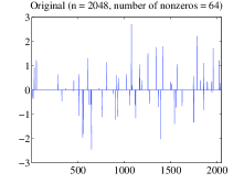
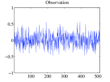
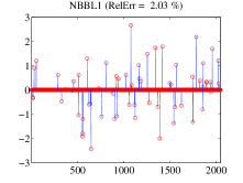
Fig. 1: Left: original signal with length $4096$ and $64$ positive non-zero elements; Middle: the noisy measurement with length $512$; Right: recovered signal by NBBL1 (red circle) versus original signal (blue peaks).

Comparing the left plot to the right one in Figure 1, we clearly see that the original sparse signal is restored almost exactly. We see that all the blue peaks are circled by the red circles, which illustrates that the original signal has been found almost exactly. All together, this simple experiment shows that our algorithm performs quite well, and provides an efficient approach to recover large sparse non-negative signal.

We have clearly known that the last term in the approximate quadratic model (2.2) is equivalent to $\|x_{k}+d\|_{1}$ exactly when $h=1$. Next, we provide evidence to show that other values can be potentially and dramatically better than $h=1$. We conduct a series of experiments and compare the performance at each case. In our experiments, we set all the parameters values as the previous test except for $n=2^{10}$. We present, in Figure 2, the impact of the parameter $h$ values on the total number of iterations, the computing time, and the quality of the recovered signal. In each plot, the level axis denotes the values of $h$ from $0.01$ to $1$ in a log scale.

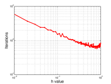
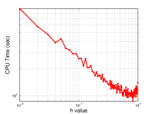
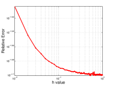
Fig. 2: Performance of NBBL1: number of iterations (left), computing time (middle) and final relative error (right). In each plot, the horizontal axis represents the value of $h$ in log scale.

In Figure 2, the number of iterations, the computing time and the quality of restorations are greatly influenced by the $h$ values. Generally, as $h$ increases, NBBL1 always has good performance. The right plot clearly demonstrates that the relative error decreases dramatically at the very beginning and then becomes slightly after $0.2$. However, the quality of restoration can not be improved any more after $0.7$. On the other hand, the left and the middle plots show that the number of iterations and the computing time slightly increase after $h=0.8$. Taking three plots together, these plots verify that the performance of NBBL1 is sensitive to the $h$ values, and the value $h\in[0.7,0.8]$ may be the better choice.

5.3 Comparisons with NESTA-Ct, GPSR-BB, CGD, TwIST and FPC-BB

The third class of the experiment is to test against several state-of-the-art algorithms which are specifically designed in recent years to solve $\ell_{1}$-regularized problems in compressive sensing or linear inverse problems. It is difficult to compare each algorithm in a very fair way, because each algorithm is compiled with different parameter settings, such as the termination criterions, the staring points, or the continuation techniques. Hence, as usual, in our performance comparisons, we run each code from the same initial point, use all the default parameter values, and only observe the convergence behavior of each algorithm to attain a similar accuracy solution.

NESTA uses Nesterov’s smoothing technique [37] and gradient method [30] to solve basis pursuit denoising problem. The current version is capable of solving $\ell_{1}$-norm regularization problems with different types including (2). In this experiment, we test NESTA with continuation (named NESTA-Ct) for comparison, where this algorithm solves a sequence of problems (2) by using a decreasing sequence of values of $\mu$. Additionally, NESTA-Ct uses the intermediated solution as a warm start for the next problem. In running NESTA, all the parameters are taken as default except TolVar is set to be $1.e-5$ to obtain similar quality solutions with others.

GPSR-BB (Gradient Projections for Sparse Reconstruction) [22] reformulates the original problem (2) as a box-constrained quadric programming problem (6) by splitting $x=u-v$. Figueiredo, Nowak and Wright use a gradient projection method with Barziali-Borwein steplength [2] for its solution. Moreover, the nonmonotone line search [24] is also used to improve its performance. For the comparison with GPSR-BB, we use its continuation variant and set all parameters as default.

The well-known CGD uses gradient algorithm to solve (5) in order to obtain the search direction $d_{k}^{i}=ze^{i}$ in $i\in\mathcal{J}$, where $\mathcal{J}$ is a nonempty subset of $\{1,...,n\}$, and choose the index subset $\mathcal{J}$ a Gauss-southwell rule. The iterative process $x_{k+1}=x_{k}+\alpha_{k}d_{k}$ continues until some termination critera are met, where $d_{k}^{i}=0$ with $i\notin\mathcal{J}$ and the stepsize $\alpha_{k}$ by using a Armijo rule. In running CGD, we use the code CGD in its Matlab package, and set all the parameter as default except for init=2 to start the iterative process at $x_{0}=A^{\top}b$.

TwIST is a two-step IST algorithm for solving a class of linear inverse problems. Specifically, TwIST is designed to solve

$$\min_{u}\mathcal{J}(u)+\frac{\mu}{2}\|Au-f\|_{2}^{2},$$ (4)

where $A$ is a linear operator, and $\mathcal{J}(\cdot)$ is a general regularizer, which can be either the $\ell_{1}$-norm or the TV. The iteration framework of TwIST is

$$u_{k+1}=(1-\alpha)u_{k-1}+(\alpha-\delta)u_{k}+\delta\Phi_{\mu}(\xi_{k}),$$

where $\alpha,\delta>0$ are parameters, $\xi_{k}=u_{k}+A^{\top}(f-Au_{k})$ and

$$\Phi_{\mu}(\xi_{k})=\text{arg}\min_{u}\mathcal{J}(u)+\frac{\mu}{2}\|u-\xi_{k}\|_{2}^{2}.$$ (5)

We use the default parameters in TwIST and terminate the iteration process when the relative variation of function value falls below $10^{-4}$.

FPC is the fixed-point continuation algorithm to solve the general $\ell_{1}$-regularized minimization problem (1), where $f$ is a continuous differentiable convex function. At current $x_{k}$ and any scalar $\tau>0$, the next iteration is produced by the so-called fixed point iteration

$$x_{k+1}=\text{sgn}(x_{k}-\tau\nabla f(x_{k}))\max\big{\{}|x_{k}-\tau\nabla f(x_{k})|-\mu\tau,0\big{\}},$$

where “sgn” is a componentwise sign function. In order to obtain a good practical performance, a continuation approach is also augmented in FPC. Moreover, the FPC is further modified by using Barzilai-Borwein stepsize (code FPC-BB in Matlab package FPC_v2). The continuation and Barzilai-Borwein stepsize techniques make FPC-BB faster than FPC. In running of FPC-BB, we use all the default parameter values except we set xtol = 1e-5 to stop the algorithm when the relative change between successive points is below xtol.

In this test, $A$ is a partial discrete cosine coefficients matrix (DCT), whose $m$ rows are chosen randomly from the $n\times n$ DCT matrix. Such encoding matrix $A$ does not require storage and enables fast matrix-vector multiplications involving $A$ and $A^{\top}$. Therefore, it is able to be used to test much larger size problems than using Gaussian matrices. In NBBL1, we take $tol_{2}=10^{-4}$, $h=0.8$, $\lambda_{(\min)}=10^{-30}$, $\lambda_{(\max)}=10^{30}$. In the line search, we choose $\tilde{\alpha}_{0}=0.8$, $\rho=0.35$, $\delta=10^{-5}$ and $\tilde{m}=5$. In this comparison, we let $n=2^{12}$, $m={\tt floor}(n/4)$. The original signal $\bar{x}$ contains $p={\tt floor}(m/6)$ number of nonzero components, where floor is a Matlab command used to round an element to the nearest integers towards minus infinity. Moreover, the observation $b$ is contaminated by Gaussian noise with level $\sigma=1e-3$. The goal is to use each algorithm to reconstruct $\bar{x}$ from the observation $b$ by solving (2) with $\mu=2^{-8}$. All the tested algorithms start at $x_{0}=A^{\top}b$ and terminate with different stopping criterions to produce similar quality resolutions. To specifically illustrate the performance of each algorithm, we draw four figures to show their convergence behavior from the point of objective function values and relative error as the iteration numbers and computing time increase, which given in Figure 3.

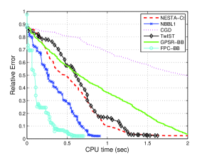
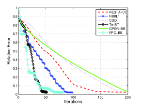
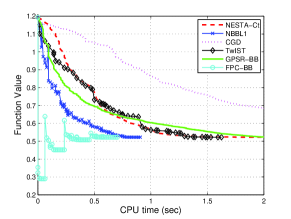
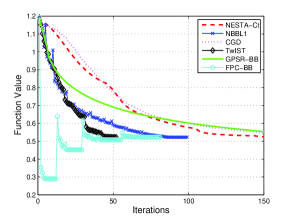
Fig. 3: Comparison result of NBBL1, NESTA-Ct, CGD, TwIST, GPSR-BB, and FPC-BB. The x-axes represent the CPU time in seconds (left column) and the number of iterations (right column). The y-axes represent the relative error (top row) and the function values (bottom row).

From the top plots in Figure 3, NBBL1 usually decreases relative errors faster than NESTA-Ct, CGD and GPSR-BB throughout the entire iteration process, and meanwhile requires less number of iterations. The top right plot shows that TwIST needs less steps than NBBL1 to obtain similar level of relative error. However, TwIST is much slower because it has to solve a de-noising subproblem (5) at each iteration. Unfortunately, NBBL1 needs further improvement to challenge the well-known code FPC-BB. We now turn our attention to observe the function values behavior of each algorithm. Similarly, NBBL1 is superior to NEST-Ct, CGD, GPSR-BB and TwIST from the computing time points of view. FPC-BB reaches the lowest function values at the very beginning, and then starts to increase it to meet nearly equal final values at the end. In this test, CGD appears to be much slower than the others, because it is sensitive to the choice of starting points. If CGD starts at $x_{0}=0$ with all the other settings unchanged, its performance should be significantly improved [40]. Taking everything together, from the limited numerical experiment, we conclude that NBBL1 provides an efficient approach for solving $\ell_{1}$-regularized nonsmooth problem and is competitive with or performs better than NESTA-Ct, GPSR-BB, CGD, TwIST and FPC-BB.

6 Conclusions

In this paper, we proposed, analyzed, and tested a new practical algorithm to solve the separable nonsmooth minimization problem consisting of a $\ell_{1}$-norm regularized term and a continuously differentiable term. The type of the problem mainly appears in signal/image processing, compressive sensing, machine learning, and linear inverse problems. However, the problem is challenging due to the non-smoothness of the regularization term. Our approach minimizes an approximal local quadratic model to determine a search direction at each iteration. The search direction reduces to the classic Barzilai-Borwein gradient method in the case of $\mu=0$. We show that the objective function is descent along this direction providing that the initial stepsize is less than $h$. We also establish the algorithm’s global convergence theorem by incorporating a nonmonotone line search technique and assuming that $f$ is bounded below. Extensive experimental results show that the proposed algorithm is an effective toll to solve $\ell_{1}$-regularized nonconvex problems from CUTEr library. Moreover, we also run our algorithm to recover a large sparse signal from its noisy measurement, and numerical comparisons illustrate that our algorithm outperforms or is competitive with several state-of-the-art solvers which specifically designed to solve $\ell_{1}$-regularized compressive sensing problems.

Unlike all the existing algorithms in this literature, our approach uses an linear model to approximate $\|x_{k}+d\|_{1}$ for computing the search direction with a small scalar $h$; that is

$$\|x_{k}+d\|_{1}\approx\|x_{k}\|_{1}+\frac{\|x_{k}+hd\|_{1}-\|x_{k}\|_{1}}{h}.$$

Although the equations may hold exactly in the case of $h=1$, a series of numerical experiments show that $h\in[0.7,0.8]$ may produce better performance with suitable experiment settings. This approach is distinctive and novel; therefore, it is one of the important contributions of this paper. As we all know, the nonmonotone Barzilai-Borwein gradient algorithm of Raydan [33] is very effective for smooth unconstrained minimization, and its remarkable effectiveness in signal reconstruction problems involving $\ell_{1}$-regularized problems has not been clearly explored. Hence, our approach can be considered as a modification or extension, to broaden the university of [33]. Moreover, the numerical experiments illustrate that our approach performs comparable to or even better than several state-of-the-art algorithms. Surely, this is the numerical contribution of our paper. Although the proposed algorithm needs further improvement to challenge the well-known code FPC-BB, the enhancement of it to deal with non-convex problems is noticeable. Our algorithm is readily to solve the $\ell_{1}$-regularized logistic regression, the $\ell_{2}$-norm and matrix trace norm minimization problems in machine learning. However, we do not test them in this paper. This should be interesting for further investigations.

References

- [1] G. Andrew and J. Gao, Scalable training of -regularized log-linear models, Proceedings of the Twenty Fourth International Conference on Machine Learning, (ICML), 2007.
- [2] J. Barzilai and J.M. Borwein, Two point step size gradient method, IMA Journal of Numerical Analysis, 8 (1988), 141-148.
- [3] A. Beck and M. Teboulle, A fast iterative shrinkage-thresholding algorithm for linear inverse problems, SIAM Journal on Imaging Science, 2 (2009), 183-202.
- [4] S. Becker, J. Bobin, and E. Candès, NESTA: A fast and accurate first-order method for sparse recovery, SIAM Journal on Imaging Science, 4 (2011), 1-39.
- [5] E. van den Berg and M.P. Friedlander, Probing the pareto frontier for basis pursuit solutions, SIAM Journal on Scientific Computing, 31 (2008), 890-912.
- [6] E.G. Birgin, J.M. Martínez, and M. Raydan, Nonmonotone spectral projected gradient methods on convex sets, SIAM Journal on Optimization, 10 (2000), 1196-1121.
- [7] J.M. Bioucas-Dias and M Figueiredo, A new TwIST: Two-step iterative shrinkage/thresholding algorithms for image restoratin, IEEE Transactions on Image Processing, 16 (2007), 2992-3004.
- [8] E.G. Birgin, J.M. Martínez, and M. Raydan, Nonmonotone spectral projected gradient methods on convex sets, SIAM Journal on Optimization, 10 (2000), 1196-1121.
- [9] J.F. Cai, E. Candès, and Z. Shen, A singular value thresholding algorithm for matrix completion, preprint, SIAM Journal on Optimization, 20 (2010), 1956-1982.
- [10] E. Candès and J. Romberg, Quantitative robust uncertainty principles and optimally sparse decompositions, Foundations of Computational Mathematics, 6 (2006), 227-254.
- [11] E. Candès, J. Romberg, and T. Tao, Stable signal recovery from imcomplete and inaccurate information, Communications on Pure and Applied Mathemathcs, 59 (2005), 1207-1233.
- [12] E. Candès, J. Romberg, and T. Tao, Robust uncertainty principles: Exact signal reconstruction from highly incomplete frequence information, IEEE Transactions on Information Theory, 52 (2006), 489-509.
- [13] E. Candès and T. Tao, Near optimal signal recovery from random projections: universal encoding strategies, IEEE Transactions on Information Theory, 52 (2004), 5406-5425.
- [14] K.W. Chang, C.J. Hsieh, and C.J. Lin, Coordinate descent method for large-scale L2-loss linear SVM, Journal of Machine Learning Research, 9 (2008), 1369-1398.
- [15] W. Cheng and D.H. Li, A derivative-free nonmonotone line search and its application to the spectral residual method, IMA J. Numer. Anal., 29 (2009), 814-825
- [16] A.R. Conn, N.I.M. Gould, Ph.L. Toint, CUTE: constrained and unconstrained testing environment, ACM Transactions on Mathematical Software, 21 (1995) 123-160.
- [17] Y.H. Dai and R. Fletcher, On the asymptotic behaviour of some new gradient methods, Mathematical Programming, 103 (2005), 541-559.
- [18] Y.H. Dai, W.W. Hager, K. Schitkowski and H. C. Zhang, The cyclic Barzilai-Borwein method for unconstrained optimization, IMA Jouornal of Numerical Analysis, 26 (2006), 1-24.
- [19] Y.H. Dai, L.Z. Liao, R-linear convergence of the Barzilai and Borwein gradient method, IMA Journal of Numerical Analysis, 26 (2002), 1-10.
- [20] D.L. Donoho, Compressed sensing, IEEE Transactions on Information Theory, 52 (2006), 1289-1306.
- [21] J. Duchi and Y. Singer, Efficient online and batch learning using forward backword splitting, Journal of Machine Learning Research, 10 (2009), 2899-2934.
- [22] M. Figueiredo, R.D. Nowak, and S.J. Wright, Gradient projection for sparse reconstruction: application to compressed sensing and other inverse problems, IEEE Journal of Selected Topics in Signal Processing, IEEE Press, Piscataway, NJ, 2007, 586-597.
- [23] A. Genkin, D.D. Lewis, and D. Madigan, Large-scale Bayesian logistic regression for text categorization, Technometrices, 49 (2007), 291-304.
- [24] L. Grippo, F. Lampariello, and S. Lucidi, A nonmonotone line search technique for Newton’s method. SIAM Journal on Numerical Analysis, 23 (1986), 707-716.
- [25] E.T. Hale, W. Yin and Y. Zhang, Fixed-point continuation for -minimization: Methodology and convergence, SIAM Journal on Optimization, 19 (2008), 1107-1130.
- [26] S. Kim, K. Koh, M. Lustig, S. Boyd, and D. Gorinevsky, An interior-point method for large-scale -regularized least squares, IEEE Journal of Selected Topics in Signal Processing, 1 (2007), 606-617.
- [27] K. Koh, S. Kim, and S. Boyd, An interior-point method for large-scale -regularized logistic regression, Journal of Machine Learning Research, 8 (2007), 1519-1555.
- [28] C.J. Lin and J.J. Moré, Newton’s method for large-scale bound constrained problems, SIAM Journal on Optimization, 9 (1999), 1100-1127.
- [29] Y. Nesterov, Smooth minimization of non-smooth functions, Mathematical Programming, 103 (2005), 127-152.
- [30] Y. Nesterov, Gradient methods for minimizing composite objective function, ECORE Discussion Paper 2007/76, available at http://www.ecore.be/DPs/dp_1191313936.pdf, 2007.
- [31] J. Nocedal, Updating quasi-Newton matrices with limited storage, Mathematices of Computation, 35 (1980), 773-782.
- [32] M. Raydan, On the Barzilai and Borwein choice of steplength for the gradient method, IMA Jouornal of Numerical Analysis, 13 (1993), 321-326.
- [33] M. Raydan, The Barzilai and Borwein gradient method for the large scale unconstrained minimization problem, SIAM Journal on Optimization, 7 (1997), 26-33.
- [34] B. Recht, M. Fazel, and P.A. Parrilo, Guaranteed minimum rank solutions of matrix equations via nuclear norm minimization, SIAM Review, 52 (2010), 471-501.
- [35] S. Shalev-Shwartz and A. Tewari, Stochastic method for l1 regularized loss minimization, In Proceedings of the Twenty Sixth International Conference on Machine Learning (ICML), 2009.
- [36] J. Shi, W. Yin, S. Osher, and P. Sajda, A fast hybrid algorithm for large-scale -regularized logistic regression, Journal of Machine Learning Research, 11 (2010), 713-741.
- [37] Y. Nesterov, Smooth minimization of non-smooth functions, Mathematical Programming, 103 (2005), 127-152.
- [38] P. Tseng and S. Yun, A coordinate gradient descent method for nonsmooth separable minimization, Mathematical Programming, 117 (2009), 387-423.
- [39] S.J. Wright, R.D. Nowak and M.A.T. Figueiredo, Sparse reconstruction by separable approximation, in roceedings of the International Conference on Acoustics, Speech, and Signal Processing, 2008, 3373-3376.
- [40] J. Yang and Y. Zhang, Alternating direction algorithms for -problems in compressive sensing, SIAM Journal on Scientific Computing, 33 (2011), 250-278.
- [41] J. Yu, S.V.N. Vishwanathan, S. Günter, and N.N. Schraudolph, A quasi-Newton approach to nonsmooth convex optimization problems in machine learning, Journal of Machine Learning Research, 11 (2010), 1145-1200.
- [42] G.X. Yuan, K.W. Chang, C.J. Hsieh, and C.J. Lin, A comparison of optimization methods and software for large-scale -regularized linear classification, Journal of Machine Learning Research, 11 (2010), 3183-3234.
- [43] S. Yun and K.C. Toh, A coordinate gradient descent method for -regularized convex minimization, Computational Optimization and Applications, 48 (2011), 273-307.
- [44] Y. Zhang, W. Sun, and L. Qi, A nonmonotone filter Barzilai-Borwein method oor optimization, Asia Pac. J. Oper. Res., 27 (2010), 55-69.