Abstract

We construct a generalized massive gravity by combining quadratic curvature gravity with the Chern-Simons term in four dimensions. This may be a candidate for the parity-odd tricritical gravity theory. Considering the AdS₄ vacuum solution, we derive the linearized Einstein equation, which is not similar to that of the three dimensional (3D) generalized massive gravity. When a perturbed metric tensor is chosen to be the Kerr-Schild form, the linearized equation reduces to a single massive scalar equation. At the tricritical points where two masses are equal to $-1$ and 2, we obtain a log-square wave solution to the massive scalar equation. This is compared to the 3D tricritical generalized massive gravity whose dual is a rank-3 logarithmic conformal field theory.

PACS numbers:

Typeset Using LaTeX

1 Introduction

Stelle [1] has first introduced the quadratic curvature gravity of $a(R_{\mu\nu}^{2}-R^{2}/3)+bR^{2}$ in addition to the Einstein-Hilbert action $R$ to improve the perturbative properties of Einstein gravity. If $ab\not=0$, the renormalizability was achieved but the unitarity was violated for $a\not=0$, indicating that the renormalizability and unitarity exclude to each other. Although the $a$-term of providing massive graviton improves the ultraviolet divergence, it induces ghost excitations which spoil the unitarity simultaneously. The price one has to pay for making the theory renormalizable in this way is the loss of unitarity. After that work, the search for a consistent quantum gravity has mainly been suffered from obtaining a renormalizable and unitary quantum field theory.

Hence, a first requirement for the quantum gravity is to gain the unitarity, which means that the classical linearized theory has no tachyon and ghost in the particle content. To that end, critical gravities have received much attention because they were considered as toy models for quantum gravity [2, 3, 4, 5, 6, 7, 8]. At the critical point, a degeneracy takes place in the AdS spacetimes and thus, ghost-like massive gravitons become massless gravitons. In this case, an equal amount of logarithmic modes should be considered for the critical gravity instead of massive gravitons. However, one has to resolve the non-unitarity problem of the log-gravity theories [3]. According to the AdS/CFT correspondence, it shows that a rank-2 logarithmic conformal field theory (LCFT) is dual to a critical gravity [9, 10, 11]. Thus, the non-unitarity of log-gravity is closely related to the non-unitarity of the LCFT which arises from the fact that the Hamiltonian cannot be diagonalized on the fields because of the Jordan structure [12, 13]. In order to avoid the non-unitarity, one has to truncate out the log-modes by imposing the AdS boundary conditions. After truncation, there remains nothing for the unitary theory.

A polycritical gravity was, recently, introduced to provide multiple critical points [14] which might be described by a higher rank LCFT. A rank of the LCFT refers to the dimensionality of the Jordan cell. For example, the LCFT dual to a critical gravity has a rank-2 Jordan cell and thus, an operator has a logarithmic partner. The LCFT dual to a tricritical gravity has rank-3 Jordan cell and an operator has two logarithmic partners. In particular, a truncation allows an odd rank LCFT to be a unitary conformal field theory (CFT) [15]. A 3D six-derivative tricritical gravity was treated as a dual to a rank-3 LCFT [16], while a four-derivative critical gravity in four dimensions was considered as a dual to a rank-3 LCFT [17]. Furthermore, it was shown that a consistent truncation of polycritical gravity may be realized at the linearized level for odd rank [18]. On the other hand, a non-linear tricritical gravity with rank-3 was investigated in three and four dimensions [19]. It is worth mentioning that a tricritical gravity was first considered in a six-derivative gravity in six dimensions [20].

Interestingly, a rank-3 and parity odd tricritical theory was considered in the context of four-derivative gravity known as three-dimensional generalized massive gravity (3DGMG) [21]. The 3DGMG is obtained by combining topologically massive gravity (TMG) [22] with new massive gravity (NMG) [23]. Two tricritical points emerged in the 3DGMG parameter space, whose dual theory is a rank-3 LCFT [24]. A truncation of the tricritical 3DGMG could be made by imposing $Q_{L}=0$ with $Q_{L}$ the Abbott-Deser-Tekin charge for log-square boundary conditions [16]. After truncation, a left-moving sector of CFT remains as a unitary theory.

At this stage, we would like to point out two related works on the 3DGMG. A log-square mode was found when choosing the Kerr-Schild metric on the AdS₃ background [25], where its dual LCFT may not be properly defined. Around the BTZ black hole background, the authors [26] have confirmed the AdS/LCFT correspondence existing between the tricritical 3DGMG and a rank-3 finite temperature LCFT by computing quasinormal frequencies of graviton approximately. However, the 3DGMG is regarded as a toy model for tricritical gravities. Hence, it is desirable to obtain a four-dimensional generalized massive gravity (4DGMG).

In this work, we wish to construct the 4DGMG by combining quadratic curvature gravity with the Chern-Simons term. Considering the AdS₄ vacuum solution together with the transverse-traceless gauge, we derive a linearized Einstein equation, which is not a compact form as found in the 3DGMG. Fortunately, taking the Kerr-Schild form for the metric perturbation, the linearized tensor equation reduces to a massive scalar equation on the AdS₄. At the tricritical points, we obtain a log-square wave solution which is similar to the solution found in the 3DGMG [25]. This is compared to the 3D tricritical GMG whose dual field theory is a rank-3 LCFT. Furthermore, we compute the linear excitation energy and conserved charges which turn out to be zero for log-square wave solutions.

2 General massive gravity in four dimensions

Before we proceed, we remind the reader that the 3DGMG is obtained by combining NMG with TMG in three dimensions. Inspired by it, we introduce the quadratic curvature gravity together with the Chern-Simons term [27, 28] in four dimensions as

$$S_{\rm 4DGMG}=\frac{1}{16\pi G}\int d^{4}x\sqrt{-g}\Big{[}R-2\Lambda+\alpha R^{2}+\beta R^{cd}R_{cd}+\frac{\theta}{4}{}^{*}RR\Big{]}$$ (2.1)

where $\Lambda$ is a cosmological constant, $\alpha$ and $\beta$ are parameters, while $\theta$ is a nondynamical field. The inclusion of $\theta$ is evident from the fact that the Pontryagin density ${}^{*}RR={}^{*}R^{a~{}cd}_{~{}b}R^{b}_{~{}acd}$ with ${}^{*}R^{a~{}cd}_{~{}b}=\frac{1}{2}\epsilon^{cdef}R^{a}_{~{}bef}$ is a total divergence [27, 28]. The $\theta$-term corresponds to a parity-violating term because it is parity odd under the parity operation: $\hat{P}[{}^{*}RR]=-[{}^{*}RR]$. We note that $\theta$ should be included as $\nabla_{c}\theta$ in the equation of motion, indicating that it may spoil the diffeomorphism symmetry [see Eq.(2.5)].

Varying for $g_{ab}$ on the action (2.1) leads to the Einstein equation

$$R_{ab}-\frac{1}{2}g_{ab}R+\Lambda g_{ab}+E_{ab}+C_{ab}=0,$$ (2.2)

where $E_{ab}$ and the 4D Cotton tensor $C_{ab}$ are given by

$$E_{ab}=\alpha\left(2RR_{ab}-\frac{1}{2}g_{ab}R^{2}+2g_{ab}\nabla^{2}R-2\nabla_{a}\nabla_{b}R\right)$$

$$+\beta\left(\frac{1}{2}g_{ab}\nabla^{2}R-\nabla_{a}\nabla_{b}R+\nabla^{2}R_{ab}+2R_{acbd}R^{cd}-\frac{1}{2}g_{ab}R_{cd}R^{cd}\right),$$ (2.3)

$$C_{ab}=\Big{(}\nabla_{c}~{}\theta~{}\epsilon^{cde}_{~{}~{}(a}\nabla_{|e|}R_{b)d}+\frac{1}{2}\nabla_{c}\nabla_{d}~{}\theta~{}\epsilon_{(b}^{~{}~{}cef}R^{d}_{~{}~{}a)ef}\Big{)}.$$ (2.4)

Here, $C_{ab}$ is a traceless and symmetric tensor. It is worth noting that applying $\nabla_{a}$ to (2.2), we get a remaining term

$$\nabla^{a}C_{ab}=-\Big{[}\frac{\nabla_{b}\theta}{8}\Big{]}~{}{}^{*}RR,$$ (2.5)

which should be zero because the Bianchi identity should be satisfied as the consistency condition. If not, a breaking of diffeomorphism-symmetry is being realized at the level of the equation of motion. For consistency, solutions of this model should satisfy ${}^{*}RR=0$ for $\nabla_{b}\theta\not=0$ since the other case of $\nabla_{b}\theta=0(C_{ab}=0)$ reduces to the quadratic curvature gravity. In this case, the diffeomorphism-symmetry could be restored dynamically. Explicitly, it could be achieved in the equation of motion by choosing the AdS₄-vacuum, even though the symmetry-breaking may occur at the action level. We note that the the same happens when $\theta$ is treated as a Lagrange multiplier.

It is easily shown that Eq.(2.2) has an AdS₄ solution

$$ds^{2}_{\rm AdS}=\bar{g}_{ab}dx^{a}dx^{b}=-\Big{(}1+\frac{r^{2}}{\ell^{2}}\Big{)}dt^{2}+\frac{dr^{2}}{1+\frac{r^{2}}{\ell^{2}}}+r^{2}d\Omega^{2}_{2}$$ (2.6)

whose geometrical quantities are given by

$$\bar{R}_{abcd}=\frac{\Lambda}{3}(\bar{g}_{ac}\bar{g}_{bd}-\bar{g}_{ad}\bar{g}_{bc}),~{}~{}~{}\bar{R}_{ab}=\Lambda\bar{g}_{ab},~{}~{}~{}\bar{R}=4\Lambda,~{}~{}~{}\Lambda=-\frac{3}{\ell^{2}}.$$ (2.7)

In order to obtain the linearized Einstein equation, we introduce the perturbation around the AdS₄ background as

$$g_{ab}=\bar{g}_{ab}+h_{ab}.$$ (2.8)

In this case, the linearized equation to (2.2) can be written as

$$\delta R_{ab}(h)-\frac{1}{2}g_{ab}\delta R(h)-\Lambda h_{ab}+\delta E_{ab}+\delta C_{ab}(h)=0,$$ (2.9)

where the linearized quantities $\delta R_{ab}(h),~{}\delta R(h),~{}\delta E_{ab}(h)$ [3] and $\delta C_{ab}(h)$ [31] are given by

$$\delta R_{ab}(h) = \frac{1}{2}\left(\bar{\nabla}^{c}\bar{\nabla}_{a}h_{bc}+\bar{\nabla}^{c}\bar{\nabla}_{b}h_{ac}-\bar{\nabla}^{2}h_{ab}-\bar{\nabla}_{a}\bar{\nabla}_{b}h\right),$$

$$\delta R(h) = \bar{\nabla}^{a}\bar{\nabla}^{b}h_{ab}-\bar{\nabla}^{2}h-\Lambda h,$$

$$\delta E_{ab}(h) = 4\Lambda\left(2\alpha+\frac{1}{3}\beta\right)\delta G_{ab}+(2\alpha+\beta)\left(g_{ab}\bar{\nabla}^{2}-\bar{\nabla}_{a}\bar{\nabla}_{b}+\Lambda g_{ab}\right)\delta R$$

$$+\beta\left(\bar{\nabla}^{2}\delta G_{ab}-\frac{2\Lambda}{3}g_{ab}\delta R\right),$$

$$\delta C_{ab}(h) = \Bigg{[}\frac{1}{2}v_{c}~{}\epsilon^{cde}_{~{}~{}~{}a}\left(\bar{\nabla}_{e}\delta R_{bd}-\Lambda\bar{\nabla}_{e}h_{bd}\right)+\frac{1}{8}v_{cd}~{}\epsilon_{b}^{~{}cef}\Big{(}\bar{\nabla}_{e}\bar{\nabla}_{f}h^{d}_{~{}a}+\bar{\nabla}_{e}\bar{\nabla}_{a}h^{d}_{~{}f}$$ (2.10)

$$-\bar{\nabla}_{e}\bar{\nabla}^{d}h_{af}-\bar{\nabla}_{f}\bar{\nabla}_{e}h^{d}_{~{}a}-\bar{\nabla}_{f}\bar{\nabla}_{a}h^{d}_{~{}e}+\bar{\nabla}_{f}\bar{\nabla}^{d}h_{ae}\Big{)}\Bigg{]}+\Bigg{[}a\leftrightarrow b\Bigg{]}$$

with

$$\delta G_{ab}=\delta R_{ab}-\frac{1}{2}\delta R\bar{g}_{ab}-\Lambda h_{ab},~{}~{}v_{c}=\bar{\nabla}_{c}\theta,~{}~{}v_{cd}=\bar{\nabla}_{c}\bar{\nabla}_{d}\theta.$$ (2.11)

Let us choose the transverse gauge as

$$\bar{\nabla}^{a}h_{ab}=\bar{\nabla}_{b}h.$$ (2.12)

Substituting (2.12) into Eq.(2.9), the trace of the linearized equation (2.9) becomes

$$\Lambda\Big{[}h-2(3\alpha+\beta)\bar{\nabla}^{2}h\Big{]}=0$$ (2.13)

when considering the traceless condition of $\delta C^{a}~{}_{a}=0$. In order to eliminate a massive spin-0 mode, we choose [3]

$$3\alpha+\beta=0.$$ (2.14)

In this case, Eq.(2.13) yields $h=0$ which implies that one may choose the transverse traceless (TT) gauge

$$\bar{\nabla}^{a}h_{ab}=0,~{}~{}~{}h=0.$$ (2.15)

Substituting (2.14) and (2.15) into (2.9) leads to

$$\frac{3\alpha}{2}\left(\bar{\nabla}^{2}-\frac{2\Lambda}{3}\right)\left(\bar{\nabla}^{2}-\frac{4\Lambda}{3}-\frac{1}{3\alpha}\right)h_{ab}+\delta C_{ab}(h)=0.$$ (2.16)

Here the linearized Cotton tensor $\delta C_{ab}(h)$ takes the complicated form

$$\delta C_{ab}(h) = \Big{[}-\frac{1}{4}v_{c}~{}\epsilon^{cde}_{~{}~{}~{}a}\bar{\nabla}_{e}\bar{\nabla}^{2}h_{bd}+\frac{\Lambda}{6}v_{c}~{}\epsilon^{cde}_{~{}~{}~{}a}\bar{\nabla}_{e}h_{bd}+\frac{1}{4}v_{cd}~{}\epsilon_{b}^{~{}cef}\Big{(}\bar{\nabla}_{e}\bar{\nabla}_{a}h^{d}_{~{}f}-\bar{\nabla}_{e}\bar{\nabla}^{d}h_{af}\Big{)}\Big{]}$$ (2.17)

$$+ \Big{[}a\leftrightarrow b\Big{]}.$$

At this stage, we point out that it is difficult to combine $\delta C_{ab}$ with the first term in (2.16) without choosing a specific form of $\theta$. It is known that for a particular $\theta$ [31, 32], one can manipulate $\delta C_{ab}$ so that the linearized equation (2.16) can be rewritten compactly. Actually, it could be achieved by choosing

$$\bar{\theta}=k\frac{x}{y},~{}~{}~{}\bar{g}_{ab}\equiv\phi^{-2}\eta_{ab}=\frac{\ell^{2}}{y^{2}}\eta_{ab}$$ (2.18)

in the Poincare coordinates $(u,v,x,y)$ for the AdS₄. Here $k$ has the dimension of [mass]^-2, $\ell$ is the AdS₄ curvature radius, and $\eta_{ab}$ is the flat metric tensor defined as

$$\eta_{ab}dx^{a}dx^{b}=2dudv+dx^{2}+dy^{2}.$$ (2.19)

Plugging (2.18) into (2.16), one arrives at

$$\Bigg{(}\bar{\nabla}^{2}-\frac{2}{3}\Lambda\Bigg{)}\Bigg{[}-3\alpha\Big{(}\bar{\nabla}^{2}-\frac{4}{3}\Lambda-\frac{1}{3\alpha}\Big{)}h_{ab}+v_{c}~{}\epsilon^{cde}_{~{}~{}~{}(a}\bar{\nabla}_{|e|}h_{b)d}\Bigg{]}=0.$$ (2.20)

Alternatively, it leads to

$$\Bigg{[}-3\alpha\Big{(}\bar{\nabla}^{2}-\frac{4}{3}\Lambda-\frac{1}{3\alpha}\Big{)}\delta_{(a}^{a^{{}^{\prime}}}\delta_{b)}^{d}+\delta_{(a}^{a^{{}^{\prime}}}v_{|c|}~{}\epsilon^{cde}_{~{}~{}~{}b)}\bar{\nabla}_{e}\Bigg{]}\Bigg{(}\bar{\nabla}^{2}-\frac{2}{3}\Lambda\Bigg{)}h_{a^{{}^{\prime}}d}=0$$ (2.21)

because two operations in Eq.(2.20) commute to each other. Here $v_{c}$ is determined by

$$v_{c}=k\Bigg{(}0,0,\frac{1}{y},-\frac{x}{y^{2}}\Bigg{)}$$ (2.22)

which may generate the mass of graviton. In this case, $v_{c}$ is not a constant vector but a vector field.

3 AdS wave as perturbation

It is a formidable task to solve (2.21) directly because the 4D Cotton term induces a complicated expression upon choosing $v_{c}$ in (2.22). In order to solve (2.21), we take the Kerr-Schild form as an AdS₄-wave solution

$$h_{ab}=2\Phi\lambda_{a}\lambda_{b},$$ (3.1)

where $\lambda_{a}=(1,0,0,0)$ is a null ($\lambda^{2}=0$) and geodesic vector and a scalar field $\Phi=\Phi(u,v,x,y)$. Additionally, the TT gauge condition (2.15) implies that one may restrict $\Phi$ to $\Phi(u,x,y)$ by taking account of the condition of $\lambda_{a}\bar{\nabla}^{a}\Phi=0$. Substituting $h_{ab}=2\Phi\lambda_{a}\lambda_{b}$ into the tensor equation (2.20) leads to the scalar equation for $\Phi$

$$\lambda_{a^{\prime}}\lambda_{d}\Big{[}-3\alpha\Big{(}\bar{\nabla}^{2}+\frac{4}{\phi}\partial^{f}\phi~{}\partial_{f}-\frac{1}{3\alpha}\Big{)}\delta_{(a}^{a^{{}^{\prime}}}\delta_{b)}^{d}+\delta_{(a}^{a^{{}^{\prime}}}v_{|c|}~{}\epsilon^{cde}_{~{}~{}~{}b)}\Big{(}\frac{\partial_{e}\phi}{\phi}+\bar{\nabla}_{e}\Big{)}\Big{]}$$

$$\hskip 170.00026pt\times\Big{[}\bar{\nabla}^{2}+\frac{2}{3}\Lambda+\frac{4}{\phi}\partial^{f}\phi~{}\partial_{f}\Big{]}\Phi=0.$$ (3.2)

Introducing the separation of variables $\Phi(u,x,y)=U(u)X(x)Y(y)$ and taking into account $\lambda_{a},~{}\phi$ in (2.18) and $v_{c}$ in (2.22), Eq.(3) reduces to

$$\Bigg{[}3\alpha\Big{(}y^{2}(\partial_{y}^{2}+\partial_{x}^{2})+2y\partial_{y}-\frac{\ell^{2}}{3\alpha}\Big{)}+k\Big{(}x\partial_{x}+y\partial_{y}+1\Big{)}\Bigg{]}$$ (3.3)

$$\hskip 130.0002pt\times\Bigg{(}y^{2}(\partial_{y}^{2}+\partial_{x}^{2})+2y\partial_{y}-2\Bigg{)}XY=0.$$ (3.4)

On the other hand, as was suggested in the 3DGMG [21], (3.3) includes two mass parameters $m_{1}$ and $m_{2}$ implicitly. In order to obtain two massive equations from (3.3), we introduce the four one-dimensional operators,

$$D^{m_{i}}=y\partial_{y}+m_{i},~{}~{}~{}D^{-1}=y\partial_{y}-1,~{}~{}~{}D^{+2}=y\partial_{y}+2$$ (3.5)

with $i=1,~{}2$. Using these mutually commuting operators, (3.3) and (3.4) can be expressed compactly as

$$D^{m_{1}}D^{m_{2}}D^{-1}D^{+2}~{}Y(y)=0\to(y\partial_{y}+m_{1})(y\partial_{y}+m_{2})(y\partial_{y}-1)(y\partial_{y}+2)~{}Y(y)=0.$$ (3.6)

In deriving this, we assume $X(x)=$constant for simplicity. Comparing Eq.(3.6) with Eq.(3.3), we find $m_{1}$ and $m_{2}$ for $\alpha\neq 0$

$$m_{1} = \frac{1}{2}\Bigg{(}1+\frac{k}{3\alpha}+\sqrt{\frac{k^{2}}{9\alpha^{2}}-\frac{2k}{3\alpha}+1+\frac{4\ell^{2}}{3\alpha}}\Bigg{)},$$ (3.7)

$$m_{2} = \frac{1}{2}\Bigg{(}1+\frac{k}{3\alpha}-\sqrt{\frac{k^{2}}{9\alpha^{2}}-\frac{2k}{3\alpha}+1+\frac{4\ell^{2}}{3\alpha}}\Bigg{)}.$$ (3.8)

For $\alpha=0$, being the Chern-Simons gravity [31], we have a third-order linearized equation from Eq.(3.3) instead of the fourth-order equation (3.6). In this case, a single mass parameter $m$ is given by either

$$m_{1}=1-\frac{\ell^{2}}{k}~{}~{}~{}{\rm or}~{}~{}~{}m_{2}=1-\frac{\ell^{2}}{k}.$$ (3.9)

4 Tricritical and critical points

Now we wish to obtain tricritical points. For this purpose, we focus on two points

$${\rm point~{}1}~{}: k=9\alpha=-3\ell^{2}~{}\Rightarrow~{}m_{1}=m_{2}=2$$ (4.1)

$${\rm point~{}2}~{}: k=-9\alpha=\frac{3}{4}\ell^{2}~{}\Rightarrow~{}m_{1}=m_{2}=-1.$$ (4.2)

For each point, (3.6) reduces to

$$D^{-1}D^{+2}D^{+2}D^{+2}~{}Y(y)=0 \Rightarrow (y\partial_{y}+2)^{3}(y\partial_{y}-1)~{}Y(y)=0$$ (4.3)

$$D^{-1}D^{-1}D^{-1}D^{+2}~{}Y(y)=0 \Rightarrow (y\partial_{y}-1)^{3}(y\partial_{y}+2)~{}Y(y)=0,$$ (4.4)

respectively. It is important to note that at the point 1, $D^{m_{1}}$ and $D^{m_{2}}$ are $D^{+2}$ [Eq.(4.3)], while at the point 2, they are $D^{-1}$ [Eq.(4.4)]. We remind the reader that these are two tricritical points, implying that there exists a three-fold degeneracy.

On the other hand, the quadratic curvature gravity [33] obtained from taking the $k=0$ limit in Eq.(3.3) has a critical point of $\alpha=\ell^{2}/6=-1/(2\Lambda)$. In this case, (3.3) and (3.4) reduce to

$$D^{-1}D^{+2}D^{-1}D^{+2}~{}Y(y)=0~{}\Rightarrow~{}(y\partial_{y}-1)^{2}(y\partial_{y}+2)^{2}~{}Y(y)=0.$$ (4.5)

In the Chern-Simons gravity which is equivalent to the $\alpha=0$ limit of (3.3) [31], we obtain two critical points of $k=\ell^{2}/2$ and $k=-\ell^{2}$ from Eq.(3.9). For each $k$, (3.3) and (3.4) become the third-order equation as

$$D^{-1}D^{-1}D^{+2}~{}Y(y)=0 \Rightarrow (y\partial_{y}+2)(y\partial_{y}-1)^{2}~{}Y(y)=0,~{}~{}~{}(k=\ell^{2}/2)$$ (4.6)

$$D^{-1}D^{+2}D^{+2}~{}Y(y)=0 \Rightarrow (y\partial_{y}-1)(y\partial_{y}+2)^{2}~{}Y(y)=0.~{}~{}~{}(k=-\ell^{2})$$ (4.7)

For $k=\ell^{2}/2$, a two-fold degeneracy emerges at $m=m_{1}=-1$, whereas there exists the other degeneracy at $m=m_{2}=2$ for $k=-\ell^{2}$.

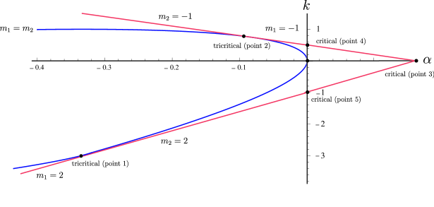
Figure 1: The tricritical and critical points in the parameter space ($\alpha,k$) for $\ell^{2}=1$. The tricritical points $1$ and $2$ correspond to $(\alpha,~{}k)=(-1/3,~{}-3)$ and $(-1/12,~{}3/4)$, respectively, while three critical points 3, 4, 5 correspond to ($1/6,~{}0$), ($0,~{}1/2$), and ($0,~{}-1$), respectively. In addition, the origin (0, 0) denotes the Einstein gravity.

Fig. 1 shows two tricritical points and three critical points in the parameter space $(\alpha,~{}k)$ of the 4DGMG. We find the solutions to Eqs.(4.3)-(4.7) for each point:

(i) $m_{1}=m_{2}=2$ $({\rm point~{}1:tricritical})$

$$\Phi(u,y) = U(u)Y(y)$$ (4.8)

$$= c_{1}(u)y+\frac{1}{y^{2}}\Big{[}c_{2}(u)+c_{3}(u)\ln(y)+c_{4}(u)\ln^{2}(y)\Big{]},$$

(ii) $m_{1}=m_{2}=-1$ $({\rm point~{}2:tricritical})$

$$\Phi(u,y) = U(u)Y(y)$$ (4.9)

$$= c_{5}(u)\frac{1}{y^{2}}+y\Big{[}c_{6}(u)+c_{7}(u)\ln(y)+c_{8}(u)\ln^{2}(y)\Big{]},$$

(iii) $m_{1}=2$, $m_{2}=-1$ $({\rm point~{}3:critical})$

$$\Phi(u,y) = U(u)Y(y)$$ (4.10)

$$= d_{1}(u)y+d_{2}(u)\frac{1}{y^{2}}+d_{3}(u)y\ln(y)+d_{4}(u)\frac{\ln(y)}{y^{2}},$$

(iv) $m_{1}=-1$, $m_{2}=0$ $({\rm point~{}4:~{}critical})$

$$\Phi(u,y) = U(u)Y(y)$$ (4.11)

$$= d_{5}(u)y+d_{6}(u)\frac{1}{y^{2}}+d_{7}(u)y\ln(y),$$

(v) $m_{1}=0$, $m_{2}=2$ $({\rm point~{}5:~{}critical})$

$$\Phi(u,y) = U(u)Y(y)$$ (4.12)

$$= d_{8}(u)y+d_{9}(u)\frac{1}{y^{2}}+d_{10}(u)\frac{\ln(y)}{y^{2}},$$

where all of $c_{i}$ and $d_{i}$ are undetermined functions of $u$.

From (i)-(v), we observe that at tricritical points $1$ and $2$, there exist log-square terms, as was shown in the tricritical 3DGMG [25], while at the critical points 3, 4, 5, the solutions have log-terms. In particular, combination of (4.11) with (4.12) yields the solution (4.10) found in the quadratic curvature gravity [33] which provides the fourth-order perturbation equation at the critical point.

5 Linearized excitation energy and conserved charges

In this section, we compute the linearized excitation energy of the log-square wave solution (3.1) with (4.8) and (4.9) to check whether the ghost state exists or not. Also, we find the conserved charges. In order to calculate the excitation energy, we first construct the bilinear Hamiltonian $H^{(2)}$. The bilinear action for the metric perturbation around the AdS₄ spacetimes is given by

$$S^{(2)} = -\frac{1}{16\pi G}\int d^{4}x\sqrt{-\bar{g}}h^{ab}\Big{[}\delta R_{ab}-\frac{1}{2}\bar{g}_{ab}\delta R-\Lambda h_{ab}+\delta E_{ab}+\delta C_{ab}\Big{]}$$ (5.1)

$$= -\frac{1}{16\pi G}\int d^{4}x\sqrt{-\bar{g}}\Big{[}\frac{3}{2}\alpha(\bar{\nabla}^{2}h^{ab})(\bar{\nabla}^{2}h_{ab})+\left(\frac{1}{2}+3\Lambda\alpha\right)(\bar{\nabla}^{c}h^{ab})(\bar{\nabla}_{c}h_{ab})$$

$$+\frac{\Lambda}{3}\left(4\Lambda\alpha+1\right)h^{ab}h_{ab}+\frac{1}{2}\epsilon^{cde}_{~{}~{}~{}a}\Big{(}v_{ce}h^{ab}\bar{\nabla}^{2}h_{bd}+v_{c}\bar{\nabla}_{e}h^{ab}\bar{\nabla}^{2}h_{bd}+\frac{2}{3}\Lambda v_{c}h^{ab}\bar{\nabla}_{e}h_{bd}\Big{)}$$

$$-\frac{1}{2}\epsilon_{b}^{~{}cef}\Big{(}v_{cde}h^{ab}\bar{\nabla}_{a}h^{d}_{~{}f}+v_{cd}\bar{\nabla}_{e}h^{ab}\bar{\nabla}_{a}h^{d}_{~{}f}-v_{cde}h^{ab}\bar{\nabla}^{d}h_{af}-v_{cd}\bar{\nabla}_{e}h^{ab}\bar{\nabla}^{d}h_{af}\Big{)}\Big{]}.$$

In deriving (5.1), we have used the transverse-traceless gauge (2.15). From the above bilinear action, the canonical momentum is defined by

$$\Pi^{ab}_{(1)} = \frac{\delta{\cal L}^{(2)}}{\delta\dot{h}_{ab}}-\bar{\nabla}_{0}\left(\frac{\delta{\cal L}^{(2)}}{\delta(d(\bar{\nabla}_{0}h_{ab})/dt)}\right)$$ (5.2)

$$= -\frac{1}{16\pi G}\sqrt{-\bar{g}}\Bigg{[}\bar{\nabla}^{0}(1+6\Lambda\alpha)h^{ab}-3\alpha\bar{g}^{00}\bar{\nabla}_{0}\bar{\nabla}^{2}h^{ab}+\frac{1}{2}\epsilon^{cd0a}v_{c}\bar{\nabla}^{2}h^{b}_{~{}d}+\frac{\Lambda}{3}v_{c}\epsilon^{ca0}_{~{}~{}~{}d}h^{db}$$

$$-\frac{1}{2}\epsilon^{bc0f}v_{cd}\bar{\nabla}^{a}h^{d}_{~{}f}-\frac{1}{2}\epsilon_{f}^{~{}ceb}v_{c}^{a}\bar{\nabla}_{e}h^{0f}+\frac{1}{2}\epsilon_{f}^{~{}ceb}v_{c~{}e}^{~{}0}h^{af}+\frac{1}{2}\epsilon^{bc0f}v_{cd}\bar{\nabla}^{d}h^{a}_{~{}f}$$

$$+\frac{1}{2}\epsilon_{f}^{~{}ceb}v_{c}^{0}\bar{\nabla}_{e}h^{af}-\frac{1}{2}\bar{\nabla}_{0}(\epsilon^{cae}_{~{}~{}~{}d}v_{c}\bar{\nabla}_{e}h^{db}\bar{g}^{00})\Bigg{]}$$

with $S^{(2)}=\int d^{4}x{\cal L}^{(2)}$. Using the Ostrogradsky formalism for a higher-order derivative Lagrangian, one defines the canonical momentum for the second-order temporal derivative as

$$\Pi^{ab}_{(2)} = \frac{\delta{\cal L}^{(2)}}{\delta(d(\bar{\nabla}_{0}h_{ab})/dt)}$$ (5.3)

$$= -\frac{1}{32\pi G}\sqrt{-\bar{g}}\bar{g}^{00}\Big{(}6\alpha\bar{\nabla}^{2}h^{ab}+\epsilon^{cae}_{~{}~{}~{}d}v_{c}\bar{\nabla}_{e}h^{db}\Big{)}.$$

Then, the bilinear Hamiltonian takes the form

$$H^{(2)}=\int d^{4}x\Big{(}\dot{h}_{ab}\Pi^{ab}_{(1)}+\frac{\partial}{\partial t}(\bar{\nabla}_{0}h_{ab})\Pi^{ab}_{(2)}\Big{)}-S^{(2)}.$$ (5.4)

Substituting Eqs.(2.18) and (3.1) into Eq.(5.4) and using $\lambda^{2}=0$ and $\lambda^{a}\bar{\nabla_{a}}\lambda_{b}=0$ leads to the vanishing Hamiltonian

$$H^{(2)}=0,$$ (5.5)

which shows that there is no ghost states for the log-square waves (4.8) and (4.9).

On the other hand, one may use the covariant formalism for 4D Chern-Simons gravity [34] and quadratic curvature gravity [4] in asymptotically AdS₄ spacetimes to derive the conserved charges in the 4DGMG as

$$Q^{a}=\int_{\cal M}dS_{i}\sqrt{-\bar{g}}\Bigg{[}{\cal A}^{ai}(\bar{\eta})+(1+2\Lambda\alpha){\cal A}^{ai}(\bar{\xi})+\alpha{\cal B}^{ai}(\bar{\xi})-\frac{1}{2}{\cal C}^{ai}(\bar{\xi})\Bigg{]},$$ (5.6)

where $\bar{\eta}^{a}=v_{b}\epsilon^{bcda}\bar{\nabla}_{d}\bar{\xi}_{c}/2$ with a Killing vector $\bar{\xi}_{c}$ and

$${\cal A}^{ai}(\bar{\xi}) = \bar{\xi}_{b}\bar{\nabla}^{a}h^{bi}-\bar{\xi}_{b}\bar{\nabla}^{i}h^{ab}+\bar{\xi}^{a}\bar{\nabla}^{i}h-\bar{\xi}^{i}\bar{\nabla}^{a}h+h^{ab}\bar{\nabla}^{i}\bar{\xi}_{b}-h^{bi}\bar{\nabla}^{a}\bar{\xi}_{b}$$

$$+\bar{\xi}^{i}\bar{\nabla}_{b}h^{ab}-\bar{\xi}^{a}\bar{\nabla}_{b}h^{ib}+h\bar{\nabla}^{a}\bar{\xi}^{i},$$

$${\cal B}^{ai}(\bar{\xi}) = -\bar{\xi}^{a}\bar{\nabla}^{i}\delta R-\delta R\bar{\nabla}^{a}\bar{\xi}^{i}+\bar{\xi}^{i}\bar{\nabla}^{a}\delta R-3\Big{(}\bar{\xi}_{b}\bar{\nabla}^{i}\delta G^{ab}-\bar{\xi}_{b}\bar{\nabla}^{a}\delta G^{bi}$$

$$-\delta G^{ab}\bar{\nabla}^{i}\bar{\xi}_{b}+\delta G^{bi}\bar{\nabla}^{a}\bar{\xi}_{b}\Big{)},$$

$${\cal C}^{ai}(\bar{\xi}) = v_{b}\bar{\xi}^{d}\epsilon^{baic}\delta G_{dc}+v_{b}\bar{\xi}_{c}\epsilon^{bcid}\delta G^{a}_{d}+v_{d}\bar{\xi}_{b}\epsilon^{dabc}\delta G^{i}_{c}.$$ (5.7)

In these expressions, $\delta R$ and $\delta G_{ab}$ are given by (2) and (2.11). Plugging (2.18) and (3.1) into (5.6) together with the Killing vector $\bar{\xi}_{a}=(1,0,0,0)/y^{2}$ and $\bar{\eta}^{a}=k\Lambda^{2}(0,1,0,0)/9$, then four quantities ${\cal A}^{ai}(\bar{\xi}),~{}{\cal A}^{ai}(\bar{\eta}),~{}{\cal B}^{ai}(\bar{\xi}),$ and ${\cal C}^{ai}(\bar{\xi})$ take simpler forms

$${\cal A}^{ai}(\bar{\xi}) = \frac{2\Phi}{y^{2}}{\cal M}^{ai},$$ (5.8)

$${\cal A}^{ai}(\bar{\eta}) = \frac{2k\Lambda^{2}\Phi}{9}{\cal M}^{ai},$$ (5.9)

$${\cal B}^{ai}(\bar{\xi}) = -\frac{3}{y^{2}}\Big{(}\bar{\nabla}^{2}\Phi-\frac{2}{3}\Lambda\Phi-\frac{4}{3}\Lambda y\Phi^{\prime}\Big{)}{\cal M}^{ai},$$ (5.10)

$${\cal C}^{ai}(\bar{\xi}) = -\frac{v_{b}}{y^{2}}\Big{(}\bar{\nabla}^{2}\Phi-\frac{2}{3}\Lambda\Phi-\frac{4}{3}\Lambda y\Phi^{\prime}\Big{)}\Big{(}\lambda^{d}\epsilon^{baic}\lambda_{d}\lambda_{c}+\lambda_{c}\epsilon^{bcid}\lambda^{a}\lambda_{d}+\lambda_{b}\epsilon^{dabc}\lambda^{i}\lambda_{c}\Big{)}.$$ (5.11)

Here the prime (^′) denotes the differentiation with respect to $y$ and ${\cal M}^{ai}$ is given by the null vector $\lambda^{a}$

$${\cal M}^{ai}=\lambda_{b}\bar{\nabla}^{a}(\lambda^{b}\lambda^{i})-\lambda_{b}\bar{\nabla}^{i}(\lambda^{a}\lambda^{b})+\lambda^{a}\lambda^{b}\bar{\nabla}^{i}\lambda_{b}-\lambda^{b}\lambda^{i}\bar{\nabla}^{a}\lambda_{b}.$$ (5.12)

In deriving these, we have used a relation of

$$\bar{\nabla}^{2}(\Phi\lambda_{a}\lambda_{b})=\Big{(}\bar{\nabla}^{2}\Phi+\frac{4}{3}\Lambda\Phi-\frac{4}{3}\Lambda y\Phi^{\prime}\Big{)}\lambda_{a}\lambda_{b}.$$ (5.13)

Employing two relations

$$\bar{\nabla}_{a}\lambda_{b} = \frac{1}{\phi}(\lambda_{a}\partial_{b}\phi+\lambda_{b}\partial_{a}\phi),$$ (5.14)

$$\bar{\nabla}_{c}(\lambda_{a}\lambda_{b}) = \frac{1}{\phi}(2\lambda_{a}\lambda_{b}\partial_{c}\phi+\lambda_{c}\lambda_{b}\partial_{a}\phi+\lambda_{c}\lambda_{a}\partial_{b}\phi),$$ (5.15)

we obtain ${\cal C}^{ai}(\bar{\xi})=0$ and ${\cal M}^{ai}=0$ which implies that ${\cal A}^{ai}(\bar{\xi})={\cal A}^{ai}(\bar{\eta})={\cal B}^{ai}(\bar{\xi})=0$. Finally, we arrive at the result that the conserved charges vanish

$$Q^{a}=0.$$ (5.16)

Before closing this section, it is worth explaining why the conserved charges vanish. It is well-known that the conserved charges of the energy and angular momentum can be obtained through the integration at spatial infinity if a timelike and a rotational Killing vector are properly given. It suggests that in our case, the conserved charges of energy and angular momentum vanish because the AdS-wave admits a nulllike Killing vector $\bar{\xi}_{c}$ only. Also we would like to mention that the zero excitation energy and zero charges are due to the following sequential restriction from tensor to scalar:

$$h_{ab}~{}~{}\xrightarrow[\rm Kerr-Schild~{}form]{}~{}~{}2\Phi\lambda_{a}\lambda_{b}~{}~{}\xrightarrow[\rm gauge-fixing]{}~{}~{}\lambda_{a}\bar{\nabla}^{a}\Phi=0.$$ (5.17)

Hence, we conjecture that all AdS-wave solutions (4.8)-(4.12) including non-critical solutions do not provide the nonzero excitation energy and conserved charges.

6 Discussions

We have constructed the generalized massive gravity by combining quadratic curvature gravity with the Chern-Simons term in four dimensions. This 4DGMG is similar to the 3DGMG. Considering the AdS₄ vacuum solution, we have derived the linearized Einstein equation, which is not a compact form compared with that of the 3DGMG. When the metric perturbation is chosen to be the Kerr-Schild form, however, the linearized tensor equation reduces to a massive scalar equation. At the tricritical points, we obtain a log-square wave solution whose dual field theory may not be properly defined. The absence of its dual LCFT is compared to the 3D tricritical GMG whose dual is a rank-3 LCFT.

A difference between the 4DGMG and 3DGMG is that the former has the Chern-Simons term of $\frac{\theta}{4}~{}^{*}RR$ with $\theta$ a nondynamical field, while the latter has the topologically massive term $\frac{1}{2\mu}\epsilon\cdot[\Gamma\partial\Gamma+\frac{2}{3}\Gamma\Gamma\Gamma]$ with $\mu$ a parameter, even though two terms belong to parity-violating term. The presence of $\theta$ in the 4DGMG may prevent us from having its dual LCFT at the tricritical point because it is not a constant like $1/\mu$ in the 3DGMG but a nondynamical field. Most of all, choosing $\theta=kx/y$ makes the linearized equation complicated on the AdS₄ spacetimes, which implies that the linearized equation (2.16) cannot be written by a compact form like as in the AdS₃ spacetimes

$$({\cal D}^{L}{\cal D}^{R}{\cal D}^{M_{+}}{\cal D}^{M_{-}}h)_{\mu\nu}=0.$$ (6.1)

Here $h_{\mu\nu}$ is the metric perturbation around the AdS₃ and operators (${\cal D}^{L/R},{\cal D}^{M_{\pm}}$) are given in [16, 21, 26]. On the other hand, the compact equation (3.6) expressed in one-dimensional operators is obtained only after choosing the AdS-wave. This implies that the parity-odd tricritical gravity theory in the 4DGMG could not be described by its dual higher rank LCFT.

However, it was discussed in the 4D quadratic curvature gravity [6] that at the critical point, the AdS-wave log solutions may provide a dual LCFT₃, while at off-critical point, its dual theory may correspond to a nonrelativistic field theory with fixed boundary conditions. It suggests that a similar thing may happen at the tricritical point and off-tricritical point in the 4DGMG. However, an explicit construction of its dual CFT is beyond the scope of the present work and thus, it is left as a future work.

Acknowledgments

This work was supported by the National Research Foundation of Korea (NRF) grant funded by the Korea government (MEST) through the Center for Quantum Spacetime (CQUeST) of Sogang University with grant number 2005-0049409. Y. Myung was partly supported by the National Research Foundation of Korea (NRF) grant funded by the Korea government (MEST) (No.2012-040499).

References

• [1] K. S. Stelle, Phys. Rev.  D 16, 953 (1977).
• [2] W. Li, W. Song and A. Strominger, JHEP 0804, 082 (2008) [arXiv:0801.4566 [hep-th]].
• [3] H. Lu and C. N. Pope, Phys. Rev. Lett.  106, 181302 (2011) [arXiv:1101.1971 [hep-th]].
• [4] S. Deser, H. Liu, H. Lu, C. N. Pope, T. C. Sisman and B. Tekin, Phys. Rev. D 83, 061502 (2011) [arXiv:1101.4009 [hep-th]].
• [5] M. Porrati and M. M. Roberts, Phys. Rev. D 84, 024013 (2011) [arXiv:1104.0674 [hep-th]].
• [6] M. Alishahiha and R. Fareghbal, Phys. Rev. D 83, 084052 (2011) [arXiv:1101.5891 [hep-th]].
• [7] E. A. Bergshoeff, O. Hohm, J. Rosseel and P. K. Townsend, Phys. Rev. D 83, 104038 (2011) [arXiv:1102.4091 [hep-th]].
• [8] H. Lu, C. N. Pope, E. Sezgin and L. Wulff, JHEP 1110, 131 (2011) [arXiv:1107.2480 [hep-th]].
• [9] D. Grumiller and N. Johansson, JHEP 0807, 134 (2008) [arXiv:0805.2610 [hep-th]].
• [10] Y. S. Myung, Phys. Lett. B 670, 220 (2008) [arXiv:0808.1942 [hep-th]].
• [11] A. Maloney, W. Song and A. Strominger, Phys. Rev. D 81, 064007 (2010) [arXiv:0903.4573 [hep-th]].
• [12] V. Gurarie, Nucl. Phys. B 410, 535 (1993) [hep-th/9303160].
• [13] M. Flohr, Int. J. Mod. Phys. A 18, 4497 (2003) [hep-th/0111228].
• [14] T. Nutma, Phys. Rev. D 85, 124040 (2012) [arXiv:1203.5338 [hep-th]].
• [15] E. A. Bergshoeff, S. de Haan, W. Merbis, M. Porrati and J. Rosseel, JHEP 1204, 134 (2012) [arXiv:1201.0449 [hep-th]].
• [16] E. A. Bergshoeff, S. de Haan, W. Merbis, J. Rosseel and T. Zojer, arXiv:1206.3089 [hep-th].
• [17] N. Johansson, A. Naseh and T. Zojer, arXiv:1205.5804 [hep-th].
• [18] A. Kleinschmidt, T. Nutma and A. Virmani, arXiv:1206.7095 [hep-th].
• [19] L. Apolo and M. Porrati, arXiv:1206.5231 [hep-th].
• [20] H. Lu, Y. Pang and C. N. Pope, Phys. Rev. D 84, 064001 (2011) [arXiv:1106.4657 [hep-th]].
• [21] Y. Liu and Y. -W. Sun, Phys. Rev. D 79, 126001 (2009) [arXiv:0904.0403 [hep-th]].
• [22] S. Deser, R. Jackiw and S. Templeton, Ann. Phys. (N.Y.)  140, 372 (1982); 185, 406(E) (1988); 281, 409 (2000).
• [23] E. A. Bergshoeff, O. Hohm and P. K. Townsend, Phys. Rev. Lett.  102, 201301 (2009) [arXiv:0901.1766 [hep-th]].
• [24] D. Grumiller, N. Johansson and T. Zojer, JHEP 1101, 090 (2011) [arXiv:1010.4449 [hep-th]].
• [25] E. Ayon-Beato, G. Giribet and M. Hassaine, JHEP 0905, 029 (2009) [arXiv:0904.0668 [hep-th]].
• [26] Y. -W. Kim, Y. S. Myung and Y. -J. Park, arXiv:1207.3149 [hep-th].
• [27] R. Jackiw and S. Y. Pi, Phys. Rev. D 68, 104012 (2003) [gr-qc/0308071].
• [28] S. Alexander and N. Yunes, Phys. Rept.  480, 1 (2009) [arXiv:0907.2562 [hep-th]].
• [29] V. Cardoso and L. Gualtieri, Phys. Rev. D 80, 064008 (2009) [Erratum-ibid. D 81, 089903 (2010)] [arXiv:0907.5008 [gr-qc]].
• [30] T. Moon and Y. S. Myung, Phys. Rev. D 84, 104029 (2011) [arXiv:1109.2719 [gr-qc]], and references therein.
• [31] T. Moon and Y. S. Myung, Eur. Phys. J. C 71, 1796 (2011) [arXiv:1108.2612 [hep-th]].
• [32] E. A.-Beato, G. Giribet, and M. Hassaine, Phys. Rev. D83, 104033 (2011) [arXiv:1103.0742 [hep-th]].
• [33] I. Gullu, M. Gurses, T. C. Sisman and B. Tekin, Phys. Rev. D 83, 084015 (2011) [arXiv:1102.1921 [hep-th]].
• [34] B. Tekin, Phys. Rev. D 77, 024005 (2008) [arXiv:0710.2528 [gr-qc]].
• [35] E. Ayon-Beato and M. Hassaine, Phys. Rev. D 73, 104001 (2006) [hep-th/0512074].