www.pnas.org/cgi/doi/10.1073/pnas.0709640104 17-07-2012 Issue Number

Submitted to Proceedings of the National Academy of Sciences of the United States of America

Imaging electronic quantum motion with light

Abstract

Imaging the quantum motion of electrons not only in real-time, but also in real-space is essential to understand for example bond breaking and formation in molecules, and charge migration in peptides and biological systems. Time-resolved imaging interrogates the unfolding electronic motion in such systems. We find that scattering patterns, obtained by X-ray time-resolved imaging from an electronic wavepacket, encode spatial and temporal correlations that deviate substantially from the common notion of the instantaneous electronic density as the key quantity being probed. Surprisingly, the patterns provide an unusually visual manifestation of the quantum nature of light. This quantum nature becomes central only for non-stationary electronic states and has profound consequences for time-resolved imaging.

TRI, time-resolved imaging; QED, quantum electrodynamics; DSP, differential scattering probability

The scattering of light from matter is a fundamental phenomenon that is widely applied to gain insight about the structure of materials, biomolecules and nanostructures. The wavelength of X-rays is of the order of atomic distances in liquids and solids, which makes X-rays a very convenient probe for obtaining real-space, atomic-scale structural information of complex materials, ranging from molecules [1] to proteins [2] and viruses [3]. The power of X-ray scattering relies as well on the fact that the X-rays interact very weakly with the electrons in matter. In a given macroscopic sample, generally no more than one scattering event per X-ray photon takes place, the probability for multiple scattering being extremely small. The key quantity in X-ray scattering is the differential scattering probability (DSP), which is related to the Fourier transform of the electronic density $\rho(\mathbf{x})$ as follows [4, 5]

$$\frac{dP}{d\Omega}=\frac{dP_{e}}{d\Omega}\left|\int d^{3}x\;\rho(\mathbf{x})~{}e^{i{\mathbf{Q}\cdot\mathbf{x}}}\right|^{2},$$ (1)

where $\frac{dP_{e}}{d\Omega}$ is the differential scattering probability from a free electron and $\mathbf{Q}$ is proportional to the momentum transfer of the scattered light. Procedures exist, for both crystalline [6] and non-crystalline samples [7], to reconstruct $\rho(\mathbf{x})$ from the scattering pattern. Equation (1) can be obtained from a purely classical description of electromagnetic radiation scattered by a stationary electron density [5], yielding a result identical to that obtained from a quantum electrodynamics (QED) description of light.

Equation (1) gives us access to a static view of the electronic density. On the other hand, much progress has been made in recent years towards understanding electronic motion with time-domain table-top experiments [8, 9, 10, 11, 12, 13], owing to the availability of laser pulses on the sub-fs time scale [14, 15]. An ultimate goal of imaging applications encompasses unraveling the motion of electrons and atoms with spatial and temporal resolutions of order 1 Å and 1 fs, respectively [16]. Recent breakthroughs make it possible to generate hard X-ray pulses of a few fs [17, 18], and pulses of length 100 as can in principle be realized [19, 20]. Hence, a fundamental question that needs to be addressed is: How does an ultrashort light pulse interact and scatter from a non-stationary quantum system?

Figure 1 shows schematically how the real-time, real-space dynamics of an electronic wave-packet can be probed by scattering a short X-ray pulse from it. In the example selected here, the electronic wavepacket is a coherent superposition of eigenstates of atomic hydrogen, with a wavepacket oscillation period of T = $6.25$ fs. The electronic dynamics of the wavepacket is probed as a function of pump-probe delay time $t$. Previously, a similar example was used to illustrate time resolved imaging of an electronic wavepacket using ultrafast electron diffraction [21]. There, the instantaneous electron density was assumed to be the main quantity being imaged.

In order to describe TRI, it is tempting to apply a similar treatment as used to obtain Eq. (1), i.e., a classical description of the X-ray pulse being scattered from a non-stationary electronic system described by the wavepacket. Therefore, under the assumption that the X-ray pulse duration is shorter than the time scale on which the motion of the electronic wavepacket unfolds (see supplementary information), the expression for the DSP becomes

$$\frac{dP}{d\Omega}=\frac{dP_{e}}{d\Omega}\left|\int d^{3}x\;\rho(\mathbf{x},t)~{}e^{i\mathbf{Q\cdot x}}\right|^{2}.$$ (2)

According to Eq. (2), TRI would be expected to provide access to the instantaneous electron density, $\rho(\mathbf{x},t)$, as a function of the delay-time $t$. The idea to assign an additional degree of freedom to the electronic density in Eq. (1), by replacing $\rho(\mathbf{x})$ with $\rho(\mathbf{x},t)$, is not new, and it has already been proposed and used in the recent past [16, 22, 23, 24]. However, a more careful consideration of the physics behind a time-resolved scattering process, quickly points to pitfalls in the simple logic underlying Eq. (2). Equation (2) implies that the scattering of light does not affect the properties of the wavepacket. But in order to image quantum motion on an ultrafast time scale, one needs an ultrashort pulse, which has an unavoidable spectral bandwidth. Due to the finite bandwidth of an ultrashort pulse, it is energetically impossible to detect whether or not in the scattering process a transition between the eigenstates spanning the wavepacket, or transitions to other states closer in energy than the pulse bandwidth, has taken place. As a result, a physically correct treatment of ultrafast imaging from the electronic wavepacket will necessarily allow for transitions among electronic states caused by the scattering process (Compton type process). In other words, it must be expected that light scattering changes the wavepacket being imaged, and that this effect will be reflected in the image. In light of this, it is questionable whether Eq. (2) is at all justified.

In the following, we apply a consistent QED description of light and a quantum mechanical description of matter. Only in this way can electronic transitions during the scattering event be properly accounted for [25, 26]. We find that the photon concept, i.e. a quantum of light scattering from the electronic system, is crucial in the description of TRI. For a sufficiently short, coherent pulse, the resulting expression for the DSP is (see supplementary information)

$$\frac{dP}{d\Omega}=\frac{dP_{e}}{d\Omega}\int d^{3}x\int d^{3}x^{\prime}\left\langle~{}\hat{n}\left(\mathbf{x}^{\prime}\right)~{}C(\hat{H})~{}\hat{n}\left(\mathbf{x}\right)~{}\right\rangle_{t}e^{i{\mathbf{Q}}\cdot(\mathbf{x}-\mathbf{x}^{\prime})}.$$ (3)

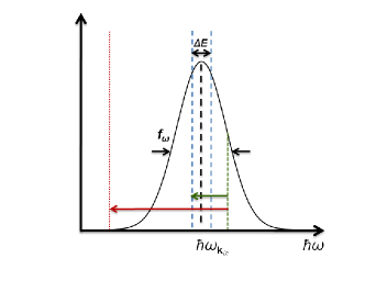
Figure 2: Schematic of the spectral energy distribution of Gaussian form of an incident ultrashort X-ray pulse with spectral bandwidth $f_{\omega}$ centered at the incident photon energy $\hbar\omega_{\mathbf{k}_{in}}$ (see supplementary information). The window function $W_{\Delta E}({\hbar\omega_{\mathbf{k}_{s}}})$ is a function of the scattered photon energy $\hbar\omega_{\mathbf{k}_{s}}$ with a width $\Delta E$ (indicated by dashed blue lines). $\Delta E$ models the range of photon energies accepted by the detector. Therefore, elastic or inelastic transitions taking place during the scattering process that fall inside $\Delta E$ are considered in the evaluation of the scattering pattern (indicated by a green arrow). Transitions falling outside the range of $\Delta E$ are not considered in the evaluation of the scattering pattern (indicated by a red arrow).

Here, $\langle~{}\cdots~{}\rangle_{t}$ is the expectation value with respect to the electronic wavepacket at delay-time $t$. The operator $C(\hat{H})=\frac{\tau~{}\Delta E}{\hbar\sqrt{\pi~{}8\ln{2}}}\exp(-\frac{\tau^{2}}{8\ln{2}~{}\hbar^{2}}(\hat{H}-\langle\hat{H}\rangle_{t})^{2})$ is a function of the electronic Hamiltonian $\hat{H}$ and of the pulse duration $\tau$. $\Delta E$ refers to the photon energy range accepted by the detector (see Fig. 2), and $\langle\hat{H}\rangle_{t}$ is the mean energy of the electronic wavepacket. $\hat{n}(\mathbf{x})$ is the electron density operator. The expectation value of $\hat{n}(\mathbf{x})$ with respect to the wavepacket at $t$ gives $\rho(\mathbf{x},t)$ i.e. $\langle\hat{n}(\mathbf{x})\rangle_{t}=\rho(\mathbf{x},t)$. As one can see from Eq. (3), the quantum description of light provides a very different expression for the TRI of the wavepacket, in comparison to that obtained from a classical description of light, Eq. (2). The crucial difference between both expressions is that Eq. (2) depends on $\langle\hat{n}(\mathbf{x}^{\prime})\rangle_{t}\langle\hat{n}(\mathbf{x})\rangle_{t}$, whereas Eq. (3) depends on $\langle~{}\hat{n}(\mathbf{x}^{\prime})~{}C(\hat{H})~{}\hat{n}(\mathbf{x})~{}\rangle_{t}$. The fingerprint of electronic transitions within the finite spectral bandwidth of the X-ray pulse is encoded in $C(\hat{H})$, which correlates the scattering of the photon at different times during the pulse duration. Similar interference effects caused by interaction of a wavepacket with a photon at different times during the pulse duration are known, for example, from fluorescence spectroscopy with optical lasers [27]. Equations (2) and (3) rely on the assumption that the transverse and longitudinal coherence lengths of the incident X-ray radiation are larger than the size of the object.

At this point it is interesting to note that many physical phenomena involving the interaction of light and matter can be explained from a classical description of light. Even the photo-electric effect can be explained by assuming classical light [28], and very sophisticated experimental scenarios such as in photon antibunching/anticorrelation experiments [29, 30] or in Lamb shift measurements  [31] are necessary to prove the quantum nature of light [32]. Surprisingly, a direct visualization of the quantum nature of light is obtained by looking at the time-resolved scattering pattern of a non-stationary quantum system. We illustrate the dramatic difference between Eqs. (2) and (3) by presenting benchmark results for TRI of the electronic wavepacket introduced in Fig. 1. Due to the inherent finite bandwidth of an ultrashort pulse, it is necessary to compute the transition amplitudes from the electronic states involved in the wavepacket to all electronic states within the bandwidth. Depending on the bandwidth, this can cover transitions to all bound states, including transitions to all Rydberg states, with any angular momentum. Therefore, the evaluation of Eq. (3) even for hydrogen is numerically challenging. In contrast, the evaluation of Eq. (2) is easy as it involves only states within the wavepacket.

Figure 3A shows scattering patterns, calculated with Eq. (3), in the $Q_{x}$ - $Q_{z}$ plane ($Q_{y}$ = 0) as a function of the delay time at times 0, T/4, T/2, 3T/4, and T. Figure 3B shows the corresponding charge distribution of the wavepacket, which undergoes spatial oscillations along the $z$-axis. The probe-pulse duration in Fig. 3A is 1 fs. A photon energy detection width, $\Delta E$, corresponding to 0.5 eV is used in the present calculation (see Fig. S1). Therefore, all transitions induced by the scattering process and resulting in a scattered photon energy within an energy range of 0.5 eV of the mean incoming photon energy were considered in the calculation of the scattering pattern. In order to ensure convergence, we considered transitions to states up to principal quantum number $n=40$. Including all types of multipole transitions allowed by the conservation of angular momentum, this amounts to about 22000 states.

As the electronic charge distribution oscillates towards the negative $z$-axis, the pattern in Fig. 3A oscillates towards positive $Q_{z}$ values. At delay times T/4 and 3T/4, the electronic charge distributions are identical, whereas the wavepacket carries a different phase, resulting in different patterns. It is evident from Fig. 3A that the scattering pattern is not at all times centrosymmetric i.e. it is not equal for $\mathbf{Q}$ and $-\mathbf{Q}$. This is in contrast with the centrosymmetric pattern expected from Eq. (2) as a consequence of Friedel’s law [33], and shown in Fig. 3C. The patterns shown in Fig. 3C were calculated using Eq. (2) with a pulse of duration 1 fs. These patterns are more intense than the patterns shown in Fig. 3A, in which the intensity depends on the photon energy detection width. It is interesting to note that the pixel with maximum intensity varies as a function of the delay-time in Fig. 3A, whereas in Fig. 3C it remains fixed at $\mathbf{Q}=0$. This counterintuitive nature of the QED scattering pattern arises from the fact that it is not simply related to the Fourier transform of the instantaneous electronic density, but it is related to the electronic wavepacket through Eq. (3). Clearly, the pattern in Fig. 3C is less rich than the correct pattern in Fig. 3A and it misses important phase information. Scattering patterns from electronic wavepackets corresponding to coherent superpositions of different sets of eigenstates (other than those used in Fig. 1) show similarly dramatic differences between Eqs. (2) and  (3). Therefore, Fig. 3A is an unusually dramatic reflection of the quantum nature of light.

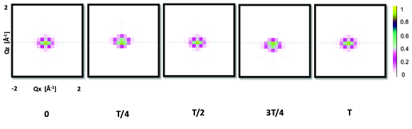
Figure 4: Scattering patterns in the $Q{{}_{x}}$ - $Q{{}_{z}}$ plane ($Q{{}_{y}}$ = 0) obtained with Eq. (3) at pump-probe delay times 0, T/4, T/2, 3T/4, and T, where the oscillation period of the electronic wavepacket is T = 6.25 fs. All the parameters used to obtain the patterns are the same as used in Fig. 3A. However, only the eigenstates belonging to the electronic wavepacket ($3d$ and $4f$ eigenstates of atomic hydrogen with angular momentum projection quantum number equal to zero) were considered. The intensities of the patterns are shown in units of $\frac{dP_{e}}{d\Omega}$.

In the illustrative example investigated here, an electronic wavepacket corresponding to the superposition of two hydrogenic eigenstates is considered. There have been several studies on the scattering of quasi-resonant light from strongly driven two-level systems [34, 35], particularly under conditions when the system is prepared initially in a superposition of states [36]. In those cases the transitions between electronic states are of dipolar nature. The TRI regime is, however, in the weak-field, one-photon limit and the photon energy is highly detuned from the energy differences between states of the wavepacket. In TRI, scattering events are Compton-like, i.e., induced by the $\mathbf{\hat{A}}^{2}$ operator (see supplementary information), and can couple electronic states over a wide range of angular momenta. In order to illustrate the difference between these scenarios, we compute scattering patterns based on Eq. (3) but restrict the calculation to the two electronic states spanning the prepared wavepacket. The patterns in Fig. 4 present an intensity similar to that in Fig. 3C because the same states are involved as in the calculation with Eq. (2). However, a careful look reveals the same periodicity and non-centrosymmetric features as seen in Fig. 3A.

Coherent diffractive imaging (CDI) [37, 38], which provides access to structural information of periodic [39] and non-periodic [40] samples, relies on the Fourier relationship between the scattering pattern and the electron density. CDI assumes Eq. (1) for a stationary electronic system, implying centrosymmetric patterns as a consequence of Friedel’s law. Consequently, the natural extension of CDI to the time domain assumes that Eq. (2) holds. On the other hand, we see that patterns obtained from a non-stationary quantum system are not centrosymmetric and cannot be related via Eq. (2) to a real function $\rho(\mathbf{x},t)$. Therefore, our results demonstrate that the extension of CDI into the time-domain requires a careful analysis of the underlying processes.

The scattering patterns calculated from Eqs. (2) and  (3) are not only unrelated, but the effect of the pulse duration in the patterns is also totally different. The respective DSPs for a particular pixel in $Q$-space for different pulse durations are shown in Fig. 5. The curve calculated with the correct description, Eq. (3), has the same periodicity as the corresponding wavepacket dynamics (Fig. 5A). In contrast, the curve calculated with Eq. (2) has the wrong periodicity (Fig. 5B). In case of pulses shorter than the characteristic time scale of the wavepacket, there is no optimal pulse duration for the signal computed with Eq. (2). The contrast as a function of time increases monotonically and for short enough pulses becomes almost constant. Conversely, the pattern computed with Eq. (3) has an optimum contrast as a function of time for a pulse length close to 1 fs. For shorter pulses, the pattern loses contrast again. The reason behind such an unexpected behavior is that in the case of hydrogen, the expectation value in Eq. (3) becomes independent of $t$ for $\tau\rightarrow 0$, intuitively because the electron has no time to change its position during $\tau$. Consequently, the pattern becomes independent of the electronic dynamics.

We have shown that TRI from a non-stationary quantum system provides visual evidence of the quantum nature of light in a very simple way. Moreover, information on the quantum motion of an electronic wavepacket beyond the instantaneous electronic density is accessed by X-ray TRI with atomic-scale spatial and temporal resolution. Our result is counterintuitive as seen from the perspective of X-ray scattering from a stationary electronic system, as one would expect to access the instantaneous electronic density for sufficiently short pulses. Not only is this not the case, but the underlying physics fundamentally differs from such an interpretation. The illustrative example used here as a proof of principle lies in the time and energy range of interest corresponding to the dynamics of valence electrons in more complex molecular and biological systems [41, 42, 43, 44]. We believe that our present findings will help to solidify the conceptual foundations of the emerging field of TRI, where understanding the motion of electrons is key to understanding the functioning of complex molecular and biological systems. The advent of novel light sources will certainly bring us closer to this goal.

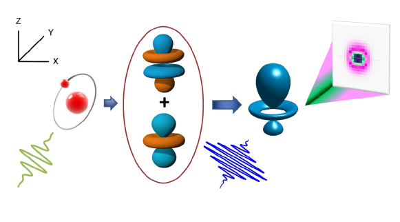
Figure 1: Schematic of the time resolved X-ray imaging scenario used as an example throughout this work. An electronic wavepacket is prepared by a laser pump pulse (indicated in green) as a coherent superposition with equal population of the $3d$ and $4f$ eigenstates of atomic hydrogen with projection of orbital angular momentum equal to zero. The polarization direction of the generated wavepacket is aligned with the laboratory $z$-axis. The electronic dynamics of the wavepacket is probed by an ultrashort X-ray pulse (indicated in blue) propagating along the $y$ direction. A series of scattering patterns obtained by varying the pump-probe time-delay serve to image the electronic motion with high spatial and temporal resolution.

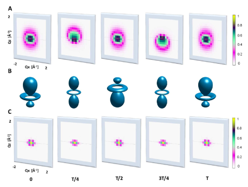
Figure 3: Scattering patterns in the $Q{{}_{x}}$ - $Q{{}_{z}}$ plane ($Q{{}_{y}}$ = 0) and electronic charge distributions of the wavepacket corresponding to the coherent superposition of $3d$ and $4f$ eigenstates of atomic hydrogen (cf. Fig. 1). (A) Scattering patterns obtained with Eq. (3), (B) electronic charge distributions and (C) scattering patterns obtained with Eq. (2), at pump-probe delay times 0, T/4, T/2, 3T/4, and T, where the oscillation period of the electronic wavepacket is T = 6.25 fs. The isosurface in (B) encloses $\sim 26\%$ of the total probability and has length 14–17 Å  along the $z$-axis and 7.5–9 Å  along the $x$ and $y$-axes. The wavepacket is exposed to a 1 fs X-ray pulse with 4 keV photons. The patterns are calculated for ${Q}_{\mathrm{max}}=2$ Å^-1 corresponding to 3.14 Å spatial resolution. For the pulse used, a real-space pixel size of 3.14 Å requires the detection of photons scattered up to 60^∘ with respect to the X-ray propagation direction, which is the $y$-axis in the present case. The grid spacing in $Q$-space is 0.19 Å^-1. The intensities of the patterns are shown in units of $\frac{dP_{e}}{d\Omega}$ in both cases.

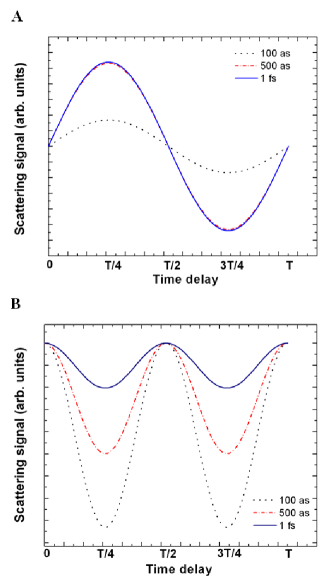
Figure 5: Effect of duration (full width at half maximum) of the X-ray pulse on the scattering patterns as a function of the pump-probe delay time. The electronic wavepacket oscillation period is T = 6.25 fs. The time evolution of the scattering pattern at an individual pixel as a function of the delay time is calculated using (A) Eq. (3), and (B) Eq. (2), for different pulse durations, 100 as (black dots), 500 as (red dash-dots), and 1 fs (blue line). In the case of the pattern calculated using Eq. (3), there is an optimal pulse duration of about 1 fs, which provides a maximum contrast as a function of time. There is no such optimum for the pattern computed with the simple expression in Eq. (2).

- [1] Ihee H, et al. (2005) Ultrafast x-ray diffraction of transient molecular structures in solution. Science 309:1223–1227.
- [2] Chapman HN, et al. (2011) Femtosecond x-ray protein nanocrystallography. Nature 470:73–77.
- [3] Seibert MM, et al. (2011) Single mimivirus particles intercepted and imaged with an x-ray laser. Nature 470:78–81.
- [4] Ashcroft NW, Mermin ND (1979) Solid State Physics (Saunders College, New York).
- [5] James RW (1982) The Optical Principles of the Diffraction of X-rays (Ox Bow, Woodbridge, Connecticut).
- [6] Hauptman HA (1991) The phase problem of x-ray crystallography. Rep. Prog. Phys. 54:1427–1454.
- [7] Miao J, Ishikawa T, Shen Q, Earnest T (2008) Extending x-ray crystallography to allow the imaging of noncrystalline materials, cells, and single protein complexes. Annu. Rev. Phys. Chem. 59:387–410.
- [8] Haessler S, et al. (2010) Attosecond imaging of molecular electronic wavepackets. Nature Physics 6:200–206.
- [9] Tzallas P, Skantzakis E, Nikolopoulos LAA, Tsakiris GD, Charalambidis D (2011) Extreme-ultraviolet pump-probe studies of one-femtosecond-scale electron dynamics. Nature Physics 7:781–784.
- [10] Hockett P, Bisgaard CZ, Clarkin OJ, Stolow A (2011) Time-resolved imaging of purely valence-electron dynamics during a chemical reaction. Nature Physics 7:612–615.
- [11] Niikura H, et al. (2002) Probing molecular dynamics with attosecond resolution using correlated wave packet pairs. Nature 421:826–829.
- [12] Goulielmakis E, et al. (2010) Real-time observation of valence electron motion. Nature 466:739–743.
- [13] Sansone G, et al. (2010) Electron localization following attosecond molecular photoionization. Nature 465:763–766.
- [14] Goulielmakis E, et al. (2008) Single-cycle nonlinear optics. Science 320:1614–1617.
- [15] Hentschel M, et al. (2001) Attosecond metrology. Nature 414:509–513.
- [16] Krausz F, Ivanov M (2009) Attosecond physics. Rev. Mod. Phys. 81:163–234.
- [17] Emma P, et al. (2010) First lasing and operation of an ångstrom-wavelength free-electron laser. Nature Photonics 4:641–647.
- [18] Pile D (2011) X-rays: First light from sacla. Nature Photonics 5:456–457.
- [19] Emma P, et al. (2004) Femtosecond and subfemtosecond x-ray pulses from a self-amplified spontaneous-emission–based free-electron laser. Phys. Rev. Lett. 92:74801.
- [20] Zholents AA, Fawley WM (2004) Proposal for intense attosecond radiation from an x-ray free-electron laser. Phys. Rev. Lett. 92:224801.
- [21] Shao HC, Starace AF (2010) Detecting electron motion in atoms and molecules. Phys. Rev. Lett. 105:263201.
- [22] Neutze R, Wouts R, van der Spoel D, Weckert E, Hajdu J (2000) Potential for biomolecular imaging with femtosecond x-ray pulses. Nature 406:752–757.
- [23] Quiney HM, Nugent KA (2011) Biomolecular imaging and electronic damage using x-ray free-electron lasers. Nature Physics 7:142–146.
- [24] Jurek Z, Oszlanyi G, Faigel G (2004) Imaging atom clusters by hard x-ray free-electron lasers. Euro. Phys. Lett. 65:491–497.
- [25] Henriksen NE, Moller KB (2008) On the theory of time-resolved x-ray diffraction. J. Phys. Chem. B 112:558–567.
- [26] Tanaka S, Chernyak V, Mukamel S (2001) Time-resolved x-ray spectroscopies: Nonlinear response functions and liouville-space pathways. Phys. Rev. A 63:63405–63419.
- [27] Scherer NF, et al. (1991) Fluorescence-detected wave packet interferometry: Time resolved molecular spectroscopy with sequences of femtosecond phase-locked pulses. J. Chem. Phys. 95:1487–1511.
- [28] Scully MO, Sargent M (1972) The concept of the photon. Physics Today 25:38–47.
- [29] Paul H (1982) Photon antibunching. Rev. Mod. Phys. 54:1061–1102.
- [30] Grangier P, Roger G, Aspect A (1986) Experimental evidence for a photon anticorrelation effect on a beam splitter: a new light on single-photon interferences. Euro. Phys. Lett. 1:173–179.
- [31] Hänsch TW, Shahin IS, Schawlow AL (1972) Optical resolution of the lamb shift in atomic hydrogen by laser saturation spectroscopy. Nature 235:63–65.
- [32] Walls DF (1979) Evidence for the quantum nature of light. Nature 280:451–454.
- [33] Als-Nielsen J, McMorrow D (2011) Elements of modern X-ray physics (Wiley New York).
- [34] Sundaram B, Milonni PW (1990) High-order harmonic generation: Simplified model and relevance of single-atom theories to experiment. Phys. Rev. A 41:6571–6573.
- [35] Eberly JH, Fedorov MV (1992) Spectrum of light scattered coherently or incoherently by a collection of atoms. Phys. Rev. A 45:4706–4712.
- [36] Gauthey FI, Keitel CH, Knight PL, Maquet A (1995) Role of initial coherence in the generation of harmonics and sidebands from a strongly driven two-level atom. Phys. Rev. A 52:525–540.
- [37] Chapman HN, Nugent KA (2010) Coherent lensless x-ray imaging. Nature Photonics 4:833–839.
- [38] Abbey B, et al. (2011) Lensless imaging using broadband x-ray sources. Nature Photonics 5:420–424.
- [39] Zuo JM, Vartanyants I, Gao M, Zhang R, Nagahara LA (2003) Atomic resolution imaging of a carbon nanotube from diffraction intensities. Science 300:1419–1421.
- [40] Miao J, Charalambous P, Kirz J, Sayre D (1999) Extending the methodology of x-ray crystallography to allow imaging of micrometre-sized non-crystalline specimens. Nature 400:342–344.
- [41] Scholes GD, Fleming GR, Olaya-Castro A, van Grondelle R (2011) Lessons from nature about solar light harvesting. Nature Chemistry 3:763–774.
- [42] Remacle F, Levine RD (2006) An electronic time scale in chemistry. Pro. Natl. Acad. Sci. USA 103:6793–6798.
- [43] Dutoi AD, Wormit M, Cederbaum LS (2011) Ultrafast charge separation driven by differential particle and hole mobilities. J. Chem. Phys. 134:024303.
- [44] Lünnemann S, Kuleff AI, Cederbaum LS (2008) Charge migration following ionization in systems with chromophore-donor and amine-acceptor sites. J. Chem. Phys. 129:104305.