Electromagnetic fluctuation-induced interactions in randomly charged slabs

Abstract

Randomly charged net-neutral dielectric slabs are shown to interact across a featureless dielectric continuum with long-range electrostatic forces that scale with the statistical variance of their quenched random charge distribution and inversely with the distance between their bounding surfaces. By accounting for the whole spectrum of electromagnetic field fluctuations, we show that this long-range disorder-generated interaction extends well into the retarded regime where higher-order Matsubara frequencies contribute significantly. This occurs even for highly clean samples with only a trace amount of charge disorder and shows that disorder effects can be important down to the nano scale. As a result, the previously predicted non-monotonic behavior for the total force between dissimilar slabs as a function of their separation distance is substantially modified by higher-order contributions, and in almost all cases of interest, we find that the equilibrium inter-surface separation is shifted to substantially larger values compared to predictions based solely on the zero-frequency component. This suggests that the ensuing non-monotonic interaction is more easily amenable to experimental detection. The presence of charge disorder in the intervening dielectric medium between the two slabs is shown to lead to an additional force that can be repulsive or attractive depending on the system parameters and can, for instance, wash out the non-monotonic behavior of the total force when the intervening slab contains a sufficiently large amount of disorder charges.

I Introduction

Patterned and heterogeneously charged materials, in particular if the heterogeneity is disorder induced, have received much attention in recent years in a number of different research areas. For instance, randomly charged polyelectrolytes rand_polyelec and patchy colloids patchy_colloids show distinct collective and thermodynamic properties than ordinary colloids and charged homopolymers DLVO ; Doi . Proteins for instance represents a prime example of biological molecules exhibiting heterogeneous and highly disordered charge distributions. The high specificity and selectivity of protein-protein interactions is one of the fundamental problems of molecular biology and requires an understanding of the interaction between randomly patterned surfaces protein . Another example which has been in the focus of recent experimental investigations is the problem of interaction between surfactant-coated surfaces which exhibit unusually strong and long-range attractive forces surf , shown to stem directly from the presence of quenched random domains (patches) of positive and negative charges on these surfaces surf_new .

In fact, most solid surfaces exhibit heterogeneous charge distributions that can be highly disordered as revealed by recent Kelvin force microscopy measurements science11 . Such random charges may result from the surface adsorption of charged contaminants and/or impurities, while even clean polycrystalline samples display patchy surface potentials barrett ; speake . The patchiness of the surface potential is believed to lead to significantly large effects in the experiments aimed at measuring the Casimir-van der Waals (vdW) interactions between solid surfaces in vacuum. Indeed, recent ultra-high sensitivity measurements have shown the presence of an “anomalously” long-range interaction which can easily mask the Casimir-vdW force at sufficiently large separations kim1 ; kim2 ; kim3 ; kim4 ; tang .

In a series of theoretical papers epl2006 ; prl2010 ; jcp2010 ; pre2011 ; epje2012 , the effects of quenched monopolar charge disorder in the bulk or surface of dielectric slabs were investigated. It was shown that even a small amount of quenched random charges can lead to strong long-range interactions between dielectric slabs. These interactions were shown to result directly from the interplay between the electrostatic interactions generated by the presence of dielectric discontinuities (the so-called image charge effects) and the quenched statistics of the random charges. It is thus remarkable to note that such forces exist even for dielectrics which are electroneutral on the average but carry a disordered charge component. In this case, net Coulomb forces are obviously absent and thus the disordered-induced forces directly compete with the Casimir-vdW forces. While the latter dominates at small separations, the former becomes substantially large and wins at large separations. The previous calculations were however performed only within the classical regime, where only the zero Matsubara frequency contributes to the Casimir-vdW force prl2010 ; jcp2010 . Strictly speaking, this approximation would be valid above the thermal wavelength (around 7 microns at room temperature) vdWgeneral , although the contribution from higher-order Matsubara frequencies would in fact dominate at much smaller separations depending on the dielectric properties of the materials (e.g., below about 1 micron in vacuum and 100 nm in a polar medium such as water ninham ). The zero-frequency results would be relevant for the large-distance regime where the above-mentioned anomalous force is observed kim1 ; kim2 ; kim3 ; kim4 ; tang . However, at sub-micron separations, it would be necessary to examine the quantum effects from the higher-order Matsubara modes of the electromagnetic field fluctuations.

In the present work, we shall thus set out to investigate in detail the interaction between two randomly charged net-neutral dielectric slabs by accounting for the full spectrum of electromagnetic field fluctuations in the following two cases: i) the slabs interact across a disorder-free dielectric continuum, considering both similar as well as dissimilar slabs, and ii) the slabs are separated in general by a dielectric layer which itself may contain random quenched charges. In both cases, the results can be compared directly against those reported previously prl2010 ; jcp2010 ; hence, we can determine the effects of the inclusion of higher-order Matsubara frequencies, which will be computed via the Lifshitz formalism vdWgeneral ; jalal , as well as the quenched disorder charges in the intervening medium.

These results thus generalize the analysis of the disorder effects to all ranges of separation down to the nano scale (as long as the continuum dielectric model employed within the Lifshitz formalism remains valid). We can then draw conclusions regarding the crossover between different scaling regimes for the interaction between slabs, which were missing from a zero-frequency analysis prl2010 ; jcp2010 . In particular, we show that the characteristic $\sim D^{-1}$ decay prl2010 of the total force with the distance $D$ between two randomly charged but otherwise (dielectrically) identical semi-infinite slabs sets in well within the retarded regime (around, e.g., 50-500 nm). Therefore, it is found that the interaction crosses over to this $\sim D^{-1}$ disorder-induced behavior from the standard (retarded) $\sim D^{-4}$ Casimir-vdW behavior rather than from the classical zero-frequency $\sim D^{-3}$ behavior. It turns out that even for highly clean samples (with disorder charge densities down to $10^{-9}\,{\mathrm{nm}}^{-3}$), the magnitude of the disorder-induced force is substantial if compared with the Casimir-vdW force.

For dielectrically dissimilar slabs, we show that the non-monotonic behavior jcp2010 of the total force as a function of distance persists when higher-order Matsubara frequencies are included. However in almost all cases, the equilibrium separation defined through the zero of total force (which can represent either a stable or unstable free energy extremum) is shifted to separations that can be substantially larger than those predicted within the zero-frequency theory jcp2010 . This is an important consequence of our analysis and suggests that the non-monotonic features of the interaction force between dielectric slabs could be easily amenable to experimental measurements in this regime tang . Such non-monotonic interaction profiles have received a lot of attention in the context of the Casimir effect in recent years and may arise in the case of metamaterials metamat and/or other exotic materials such as topological insulators topol , as well as in certain non-trivial geometries geom_casimir ; sernelius . In our analysis the $\sim D^{-1}$ behavior of the interaction force for identical slabs and the non-monotonic force profile for dissimilar slabs represent characteristic fingerprints of the charge disorder and can thus be useful in assessing whether the experimentally observed interactions in ordinary dielectrics can be interpreted in terms of disorder effects.

The organization of the paper is as follows: In Section II, we introduce our model and the details of the formalism employed in our analysis. The results for two semi-infinite slabs interacting across vacuum or a disorder-free dielectric layer are discussed in Section III.1 and those for the case where the slabs interacting across a dielectric layer which itself contains disordered charges is discussed in Section III.2. We conclude our study in Section IV.

II Model and Formalism

We consider a plane-parallel three-slab system consisting of two semi-infinite regions of dielectric response functions $\epsilon_{1}(\omega)$ and $\epsilon_{2}(\omega)$ and an intervening slab of thickness $D$ and dielectric response function $\epsilon_{m}(\omega)$ (see Fig. 1). All three slabs are assumed to carry a disordered monopolar charge distribution, $\rho(\mathbf{r})$ note_gs . The disordered charge distribution is taken to have a zero mean value $\langle\!\langle\rho(\mathbf{r})\rangle\!\rangle=0$, which ensures that the slabs are net-neutral, and a two-point correlation function

$$\langle\!\langle\rho(\mathbf{r})\rho(\mathbf{r}^{\prime})\rangle\!\rangle={\mathcal{G}}({\bm{\varrho}}-{\bm{\varrho}}^{\prime};z)\delta(z-z^{\prime}),$$ (1)

where $\langle\!\langle\cdots\rangle\!\rangle$ denotes the average over all realizations of the charge disorder distribution, $\rho(\mathbf{r})$. Here, ${\bm{\varrho}}=(x,y)$ denotes the lateral directions in the plane of the slab perpendicular to the $z$ axis where the bounding surfaces are taken to be located at $z=\pm D/2$. The above form of the correlation function thus implies no spatial correlations in $z$ direction and can be thus applicable in general to layered materials. In lateral directions, we have a statistically invariant correlation function whose specific form may depend on $z$, i.e.

$${\mathcal{G}}({\bm{\varrho}}-{\bm{\varrho}}^{\prime};z)=g(z)c({\bm{\varrho}}-{\bm{\varrho}}^{\prime};z),$$ (2)

where

$$c({\mathbf{x}};z) = \left\{\begin{array}[]{ll}c_{1}({\mathbf{x}})&\quad z<-D/2,\\ c_{m}({\mathbf{x}})&\quad|z|<D/2,\\ c_{2}({\mathbf{x}})&\quad z>D/2,\end{array}\right.$$ (6)

and we shall further assume that the disorder variance $g(z)$, which gives the density of random quenched charges in the bulk of the slabs prl2010 , is given by

$$g(z) = \left\{\begin{array}[]{ll}g_{1}e_{0}^{2}&\quad z<-D/2,\\ g_{m}e_{0}^{2}&\quad|z|<D/2,\\ g_{2}e_{0}^{2}&\quad z>D/2.\end{array}\right.$$ (10)

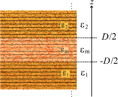
Figure 1: (Color online) We consider two semi-infinite net-neutral regions with dielectric response functions $\epsilon_{1}(\omega)$ and $\epsilon_{2}(\omega)$ with the static dielectric constants, $\varepsilon_{1}$ and $\varepsilon_{2}$, respectively, and monopolar charge disorder distributions (shown schematically by small light and dark patches) described with variances $g_{1}$ and $g_{2}$. The intervening slab may be either vacuum or in general a net-neutral dielectric material of thickness $D$ and dielectric response function $\epsilon_{m}(\omega)$ with the static dielectric constant of $\varepsilon_{m}$ and charge disorder of variance $g_{m}$.

We shall not deal with effects due to disorder in the dielectric response of the interacting media randomdean1 ; randomdean2 , which presents an additional source of disorder meriting further study and focus only on quenched disorder (see Refs. epl2006 ; prl2010 ; jcp2010 ; mama ; pre2005 for the cases studied with annealed or partially annealed disorder, or with mobile ions on or in between the randomly charged surfaces on the zero-frequency level). The quenched model is an idealization of the real nature of random charge distributions that can in general exhibit dynamical behavior, but these effects are expected to be small since ion relaxation processes are extremely slow on the scale of the Matsubara frequencies.

We base our analytical calculations on no other assumption regarding the lateral correlation function, so the expressions in what follows may be applied straightforwardly to some rather general cases, such as disorder distributions with a “patchy” structure characterized by a lateral correlation function decaying over a finite correlation length jcp2010 . Although, for the sake of brevity, we restrict our final discussion in this paper to the case where the disorder distribution is statistically homogeneous and uncorrelated, $c({\bm{\varrho}}-{\bm{\varrho}}^{\prime};z)=\delta({\bm{\varrho}}-{\bm{\varrho}}^{\prime})$, thus

$$\langle\!\langle\rho(\mathbf{r})\rho(\mathbf{r}^{\prime})\rangle\!\rangle=g(z)\delta(\mathbf{r}-\mathbf{r}^{\prime}).$$ (11)

In our previous works, we derived the partition function of the system defined above for the case where the intervening medium is free from any kind of charge disorder and the electromagnetic field fluctuations are taken into account only on the zero-frequency level prl2010 ; jcp2010 . The latter would be a valid approximation only at sufficiently large separation distances, $D$, or sufficiently high temperatures, $T$. In the present work, we shall account for all higher-order Matsubara modes of the electromagnetic field fluctuations, which become increasingly important at small separations down to the nano scale. It is easy to see that when the disorder is perfectly quenched, as indeed we assume here, these charge sources only couple to the zero-frequency mode and thus do not mix with the higher-order frequency modes of the electromagnetic field fluctuations. We do not delve further into the details of the derivation of the free energy of the quenched system, which can be written, after averaging over various realizations of the charge disorder (see Ref. jcp2010 for details), in an additive form as

$${\mathcal{F}}={\mathcal{F}}_{\mathrm{vdW}}+{\mathcal{F}}_{\mathrm{dis}}.$$ (12)

The first term on the right hand side above is the Casimir-vdW interaction free energy, which is obtained in the Lifshitz form of the surface free energy density as

$$\frac{\beta{\mathcal{F}}_{\mathrm{vdW}}}{S} = \sum_{\bf Q}{\sum_{n=0}^{\infty}}^{\prime}\ln\bigg{[}1-\Delta^{({\mathrm{TM}})}_{2,m}(\imath\xi_{n})\Delta^{({\mathrm{TM}})}_{1,m}(\imath\xi_{n})\times$$ (13)

$$\times\,e^{-2D\kappa_{m}(\imath\xi_{n})}\bigg{]}+~{}[({\mathrm{TM}})\rightarrow({\mathrm{TE}})],$$

where $k_{\mathrm{B}}T=1/\beta$ and $S$ is the surface area of the slabs. The free energy is normalized in such a way that it tends to zero at infinite separation distance $D$ and TM and TE correspond to transverse magnetic and transverse electric modes. In the Lifshitz formula the $\bf Q$ summation is over the transverse wave vector and the $n$ summation (where the prime indicates that the $n=0$ term has a weight of $1/2$) is over the imaginary Matsubara frequencies

$$\xi_{n}=\frac{2\pi nk_{\mathrm{B}}T}{\hbar},$$ (14)

where $\hbar$ is the Planck constant divided by $2\pi$. All the quantities in the bracket depend on $\bf Q$ as well as $\xi_{n}$. We have defined

$$\Delta^{({\mathrm{TM}})}_{\alpha,\beta}(\imath\xi_{n})=\frac{\epsilon_{\alpha}(\imath\xi_{n})\kappa_{\beta}(\imath\xi_{n})-\epsilon_{\beta}(\imath\xi_{n})\kappa_{\alpha}(\imath\xi_{n})}{\epsilon_{\alpha}(\imath\xi_{n})\kappa_{\beta}(\imath\xi_{n})+\epsilon_{\beta}(\imath\xi_{n})\kappa_{\alpha}(\imath\xi_{n})},$$ (15)

which quantify the dielectric mismatch across the bounding surfaces between the three different slabs labeled by $\alpha,\beta=1,m,2$. Also $\kappa_{\alpha}(\imath\xi_{n})$ for each electromagnetic field mode within the slab $\alpha$ is given by

$$\kappa_{\alpha}^{2}(\imath\xi_{n})=Q^{2}+\frac{\epsilon_{\alpha}(\imath\xi_{n})\mu_{\alpha}(\imath\xi_{n})\xi_{n}^{2}}{c^{2}},$$ (16)

where $c$ is the speed of light in vacuo, $Q$ is the magnitude of the transverse wave vector, and $\epsilon_{\alpha}(\imath\xi_{n})$ and $\mu_{\alpha}(\imath\xi_{n})$ are the dielectric response function and the magnetic permeability of the corresponding slab at imaginary Matsubara frequencies, respectively. For the sake of simplicity we assume that for all slabs $\mu_{\alpha}(\imath\xi_{n})=1$. Note that $\epsilon(\imath\xi)$ is standardly referred to as the vdW-London dispersion transform of the dielectric function and follows as Wooten

$$\epsilon(\imath\xi)=1+\frac{2}{\pi}\int_{0}^{\infty}\frac{\omega\,{\mathrm{Im}}[\epsilon(\omega)]}{\omega^{2}+\xi^{2}}\,d\omega,$$ (17)

being in general a real, monotonically decaying function of the imaginary argument $\xi$ vdWgeneral ; ninham .

For the TE modes everything remains the same except that in this case

$$\Delta^{({\mathrm{TE}})}_{\alpha,\beta}(\imath\xi_{n})=\frac{\kappa_{\beta}(\imath\xi_{n})-\kappa_{\alpha}(\imath\xi_{n})}{\kappa_{\beta}(\imath\xi_{n})+\kappa_{\alpha}(\imath\xi_{n})}.$$ (18)

The general contribution from disorder charges follows in an exact form as jcp2010

$${\mathcal{F}}_{\mathrm{dis}} = {\textstyle{\frac{1}{2}}}\int\!{\mathrm{d}}{\mathbf{r}}\,{\mathrm{d}}{\mathbf{r}}^{\prime}\,{\mathcal{G}}({\bm{\varrho}}-{\bm{\varrho}}^{\prime};z)\delta(z-z^{\prime})G({\mathbf{r}},{\mathbf{r}}^{\prime})=$$ (19)

$$={\textstyle{\frac{1}{2}}}\int\!{\mathrm{d}}{\mathbf{r}}\,{\mathrm{d}}{\mathbf{r}}^{\prime}\,g(z)c({\bm{\varrho}}-{\bm{\varrho}}^{\prime};z)\delta(z-z^{\prime})G({\mathbf{r}},{\mathbf{r}}^{\prime}).$$

where $G({\mathbf{r}},{\mathbf{r}}^{\prime})$ is the zero-frequency (electrostatic) Green’s function defined via

$$\varepsilon_{0}\nabla\cdot[\varepsilon(\mathbf{r})\nabla G(\mathbf{r},\mathbf{r}^{\prime})]=-\delta(\mathbf{r}-\mathbf{r}^{\prime}),$$ (20)

for the zero-frequency or static dielectric constant profile defined as

$$\varepsilon({\mathbf{r}}) = \left\{\begin{array}[]{ll}\varepsilon_{1}\equiv\epsilon_{1}(0)&\quad z<-D/2,\\ \varepsilon_{m}\equiv\epsilon_{m}(0)&\quad|z|<D/2,\\ \varepsilon_{2}\equiv\epsilon_{2}(0)&\quad z>D/2.\end{array}\right.$$ (24)

Equation (19) is valid for any arbitrary disorder correlation function ${\mathcal{G}}({\bm{\varrho}}-{\bm{\varrho}}^{\prime};z)$ and dielectric constant profile $\varepsilon({\mathbf{r}})$. For the particular plane-parallel three-slab model considered in this work, the Green’s function $G({\mathbf{r}},{\mathbf{r}}^{\prime})$ can be calculated from standard methods and one finds

$$\frac{\beta{\mathcal{F}}_{\mathrm{dis}}}{S} = -l_{\mathrm{B}}\int\!\frac{{\mathrm{d}}Q}{Q}\frac{e^{-2QD}}{1-\Delta_{1}\Delta_{2}\,e^{-2QD}}\bigg{[}\frac{\varepsilon_{m}g_{1}c_{1}(Q)}{(\varepsilon_{1}+\varepsilon_{m})^{2}}\,\Delta_{2}+$$ (25)

$$\!+\frac{\varepsilon_{m}g_{2}c_{2}(Q)}{(\varepsilon_{2}+\varepsilon_{m})^{2}}\Delta_{1}\!-\!\frac{\varepsilon_{1}g_{m}c_{m}(Q)}{(\varepsilon_{1}+\varepsilon_{m})^{2}}\Delta_{2}\!-\!\frac{\varepsilon_{2}g_{m}c_{m}(Q)}{(\varepsilon_{2}+\varepsilon_{m})^{2}}\Delta_{1}\!\bigg{]},$$

for arbitrary separation distance $D$, where

$$\Delta_{i}=\frac{\varepsilon_{i}-\varepsilon_{m}}{\varepsilon_{i}+\varepsilon_{m}}\qquad\quad i=1,2,$$ (26)

is the static dielectric jump parameter at each of the bounding surfaces at $z=\pm D/2$, and

$$l_{\mathrm{B}}=\beta e_{0}^{2}/(4\pi{\varepsilon_{0}})$$ (27)

is the Bjerrum length in vacuum ($l_{\mathrm{B}}\simeq 56.8$ nm at room temperature), and $c_{\alpha}(Q)$ is the Fourier transform of the correlation function $c_{\alpha}({\mathbf{x}})$. As noted before, we shall focus here on the particular case with no spatial correlations, see Eq. (11), corresponding to $c_{\alpha}(Q)=1$ for all three slabs $\alpha=1,m,2$.

Note that ${\mathcal{F}}_{\mathrm{dis}}$ stems from electrostatic interactions between randomly distributed disorder charges in the three slabs. Due to the dielectric discontinuities across the two bounding surfaces, each disorder charge is accompanied by an infinite number of electrostatic “images”, which are in fact generated by the (static) polarization of the slabs. These “image” charges also contribute to the total free energy of the system as they interact among themselves and with the actual disorder charges. This type of effects are systematically taken into account through the electrostatic Green’s function $G({\mathbf{r}},{\mathbf{r}}^{\prime})$ and are completely included in the above disorder free energy jcp2010 .

Our goal is to calculate the effective interaction force $f$, which is mediated between slabs 1 and 2 by both the electromagnetic field fluctuations and the disorder charges placed in the intervening slab, or equivalently the effective interaction free energy ${\mathcal{F}}$ between the two bounding surfaces at $z=\pm D/2$, i.e.

$$f=-\frac{\partial{\mathcal{F}}}{\partial D}\qquad{\mathrm{with}}\qquad{\mathcal{F}}(D)={\mathcal{F}}_{\mathrm{vdW}}(D)+{\mathcal{F}}_{\mathrm{dis}}(D),$$ (28)

which can thus be calculated in an explicit form from Eqs. (13) and (25).

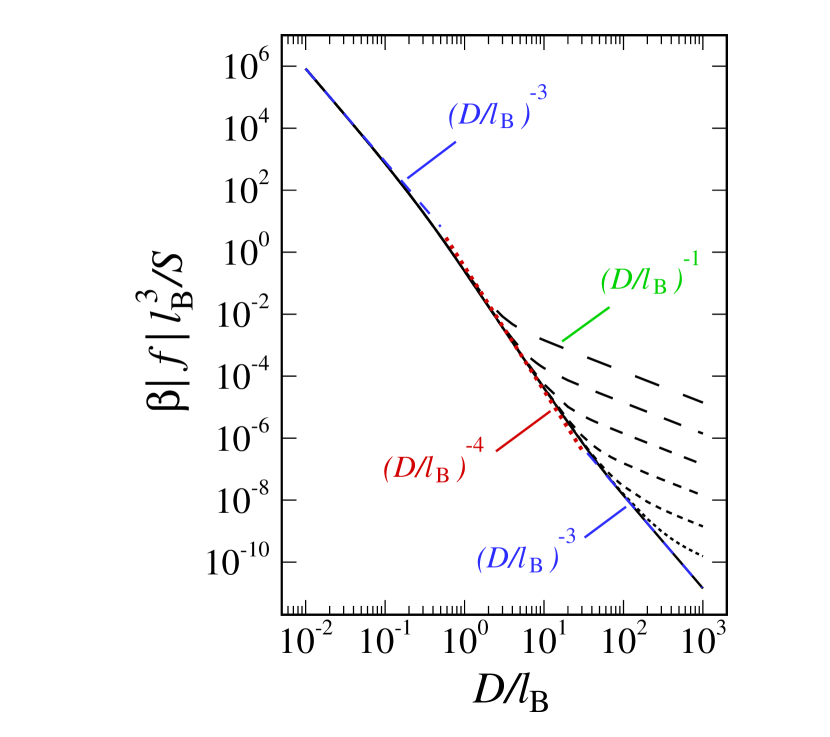
(a)

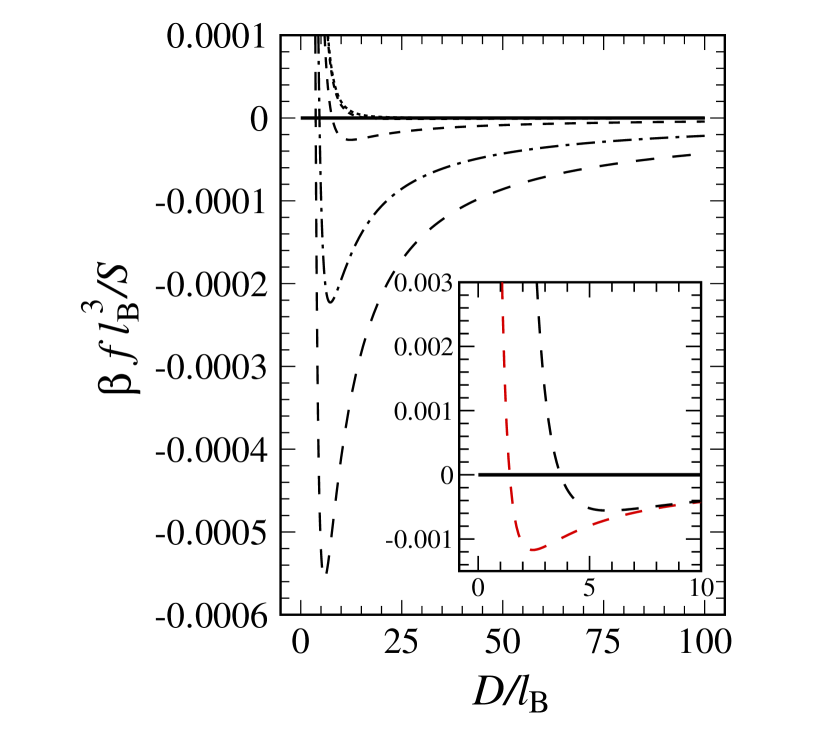
(b)

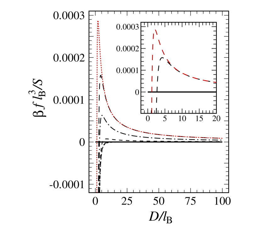
(c)

Figure 2: (Color online) (a) Magnitude of the rescaled total force, $\beta|f|l_{\mathrm{B}}^{3}/S$, between two identical semi-infinite and net-neutral dielectric slabs in vacuum ($\varepsilon_{m}=1$) is plotted on a log-log scale as a function of the rescaled distance, $D/l_{\mathrm{B}}$ (see Eq. (28)). The dielectric response function is taken according to Eq. (29) with $\varepsilon_{1}=\varepsilon_{2}=3.81$, which is appropriate for SiO₂ (see the text for other parameters). The bulk disorder variance is varied in the range $g_{1}=g_{2}=10^{-6},10^{-7},10^{-8},10^{-9},10^{-10},10^{-11}\,{\mathrm{nm}}^{-3}$ (from top to bottom). Solid curve shows the pure Casimir-vdW force obtained from Eq. (13). The scaling behavior of the free energy in various regimes of separation is shown explicitly. (b) The rescaled total force, $\beta fl_{\mathrm{B}}^{3}/S$ between two dissimilar net-neutral slabs when the dielectric response functions satisfy the relationship $\epsilon_{1}(\imath\xi)<\epsilon_{m}(\imath\xi)<\epsilon_{2}(\imath\xi)$ with the static dielectric constant values $\varepsilon_{1}=5$, $\varepsilon_{m}=10$ and $\varepsilon_{2}=50$. Here we assume $g_{m}=0$ and $g_{1}=g_{2}=10^{-6},5\times 10^{-7},10^{-7},10^{-8},10^{-10}\,{\mathrm{nm}}^{-3}$ (from bottom to top). Inset shows a closer view of the region around the minimum for $g_{1}=g_{2}=10^{-6}\,{\mathrm{nm}}^{-3}$, compared with the results obtained by including only the zero-frequency contribution (red curve). (c) Same as (b) but here we take $\epsilon_{1}(\imath\xi),\epsilon_{2}(\imath\xi)<\epsilon_{m}(\imath\xi)$ with the static dielectric constant values $\varepsilon_{1}=15$, $\varepsilon_{m}=30$ and $\varepsilon_{2}=25$.

III Results

III.1 Role of higher-order Matsubara frequencies

In order to bring out the role of higher-order Matsubara frequencies and compare it with our previous zero-frequency results jcp2010 , we shall first proceed by taking two slabs interacting across vacuum or a disorder-free dielectric medium with $g_{m}=0$. We consider three different cases: two identical slabs with $\epsilon_{1}(\imath\xi)=\epsilon_{2}(\imath\xi)$ in vacuum and two dissimilar slabs with $\epsilon_{1}(\imath\xi)<\epsilon_{m}(\imath\xi)<\epsilon_{2}(\imath\xi)$ and $\epsilon_{1}(\imath\xi),\epsilon_{2}(\imath\xi)<\epsilon_{m}(\imath\xi)$. In order to enable a direct comparison between these different cases, we assume a simple model for the vdW-London dispersion transform of the dielectric response functions of the slabs as ninham

$$\epsilon(\imath\xi)=1+\frac{C_{1}\omega_{1}^{2}}{\xi^{2}+\omega_{1}^{2}}+\frac{C_{2}\omega_{2}^{2}}{\xi^{2}+\omega_{2}^{2}},$$ (29)

in all cases. This form for the vdW-London dispersion transform mimics two characteristic relaxation mechanisms in the materials (e.g., one due to electronic polarization and the other due to ionic polarization as is the case for SiO₂ Hough ). The parameters $C_{1}$, $C_{2}$, $\omega_{1}$ and $\omega_{2}$ are chosen such that the required inequality relationships between different dielectric response functions at all Matsubara frequencies as well as the desirable values for the zero-frequency dielectric constants are obtained. These values are given in Table 1 and are not meant to represent any specific material. The qualitative aspects of our results do not depend on the particular values for these parameters but on the relationships between dielectric response functions of the slabs as discussed throughout the text. All calculations that follow are done at room temperature $T=300~{}\mathrm{K}$.

$\varepsilon\equiv\epsilon(0)$	$C_{1}$	$C_{2}$
3.81 (SiO2)	1.098	1.703
5	1	3
10	3	6
15	5	9
25	9	15
30	11	18
40	14	25
50	20	29
60	24	35
100	34	65

Table 1: Parameter values for the coefficients $C_{1}$ and $C_{2}$ in the vdW-London dispersion transform of the dielectric response function (29) are chosen in such a way that the static dielectric constants, $\varepsilon\equiv\epsilon(0)$, shown on the left column are reproduced. In all cases, we fix the characteristic frequencies as $\omega_{1}=2.033\times 10^{16}$ rad/s and $\omega_{2}=1.88\times 10^{14}$ rad/s.

Let us first consider the case of two identical slabs with equal charge disorder densities, $g_{1}=g_{2}=g$, in vacuum. In this case, we choose the parameters in Eq. (29) appropriate for SiO₂, i.e., $C_{1}$ = 1.098, $C_{2}$ = 1.703, $\omega_{1}=2.033\times 10^{16}$ rad/s, and $\omega_{2}=1.88\times 10^{14}$ rad/s Hough . The static dielectric constant of SiO₂ is thus obtained as $\epsilon(0)=3.81$.

For very low disorder variance, the Casimir-vdW interaction dominates and thus the total force between the slabs in vacuum is expected to follow the standard Lifshitz form for neutral dielectrics and thus go from the non-retarded form characterized by the power-law decay $\sim D^{-3}$ at small separations, through the retarded form $\sim D^{-4}$ for larger separations and then back to the zero-frequency form which for asymptotically large separations scales again as $\sim D^{-3}$. This behavior is shown in Fig 2a. Here we change the disorder variance in the range from $g_{1}=g_{2}=10^{-11}$ up to $10^{-6}$ nm^-3 Kao_Pitaevskii , showing clearly that the disorder effects set in for this range of parameters for separations larger than about 50 nm. This is well into the retarded regime and is thus beyond the regime where the simple zero-frequency results jcp2010 can be valid. However, once the disorder effects set in, they quickly dominate and the interaction force shows the characteristic power-law decay $\sim D^{-1}$ prl2010 . Note that the magnitude of the total force can increase by orders of magnitude as compared with the pure Casimir-vdW force (Fig 2a). Also the transitions between various power-law regimes may depend crucially on the characteristics of the dielectric spectra and may be quite complicated for different real materials.

For identical slabs in vacuum both the Casimir-vdW force as well as the disorder-induced force are attractive. When the slabs are dissimilar, one may encounter more interesting cases where the two effects oppose each other jcp2010 . We now consider a situation where $\epsilon_{1}(\imath\xi)<\epsilon_{m}(\imath\xi)<\epsilon_{2}(\imath\xi)$ and again only the two semi-infinite slabs carry disorder charges ($g_{m}=0$). In this case, the pure Casimir-vdW force is known to be repulsive vdWgeneral ; vdw_repulsive ; sernelius2 but the disorder force may be repulsive or attractive depending on the static dielectric constants jcp2010 . In Fig. 2b, we show the results for a case where the disorder force is in fact attractive and thus for sufficiently large disorder variances in the slabs, one obtains a non-monotonic behavior for the total force as a function of the separation, $D$. Such a non-monotonic behavior is one of the most remarkable features of the interactions between neutral but randomly charged dielectrics. Non-monotonic fluctuation-induced interactions between (neutral) materials have received a lot of attention in recent years metamat ; topol ; geom_casimir ; sernelius . The presence of a small amount of quenched random charges can thus provide another mechanism that can lead to non-monotonic interactions when dielectric slabs interact across a dielectric medium.

Note that there is an equilibrium separation distance, $D_{0}$, where the total force vanishes, which, in the present case, represents a stable equilibrium separation between the slabs (Fig. 2b). Thus, the disorder effects give rise to a bound state between neutral slabs which otherwise tend to repel each other due to the Casimir-vdW forces. On the other hand, we find a maximum attractive force at slightly larger separations than $D_{0}$. This may be used to optimize the thickness of the intervening medium in order to achieve the maximum force magnitude between the slabs. The remarkable point is that, the zero-frequency calculation jcp2010 (red dashed line in the inset of Fig. 2b) significantly underestimates the value of the the bound-state separation; it gives a value of $D_{0}\simeq 1.4l_{\mathrm{B}}\simeq 79.5$ nm, while the inclusion of higher-order frequencies (black dashed line in the inset of Fig. 2b) yields $D_{0}\simeq 3.4{\ell_{\mathrm{B}}}\simeq 193.1$ nm for $g_{1}=g_{2}=10^{-6}$ nm^-2 and the parameter values specified in the figure (inset). Hence, a systematic calculation of the Casimir-vdW force based on higher-order Matsubara frequencies predicts that the above-mentioned non-monotonic behavior can occur in a regime which is even more easily accessible to experimental verification tang than the prediction within the zero-frequency calculation jcp2010 . In the regime that the non-monotonic behavior is found, the magnitude of the total force in the presence of disorder is typically much larger than the pure Casimir-vdW force as may be seen from Figs. 2b and c.

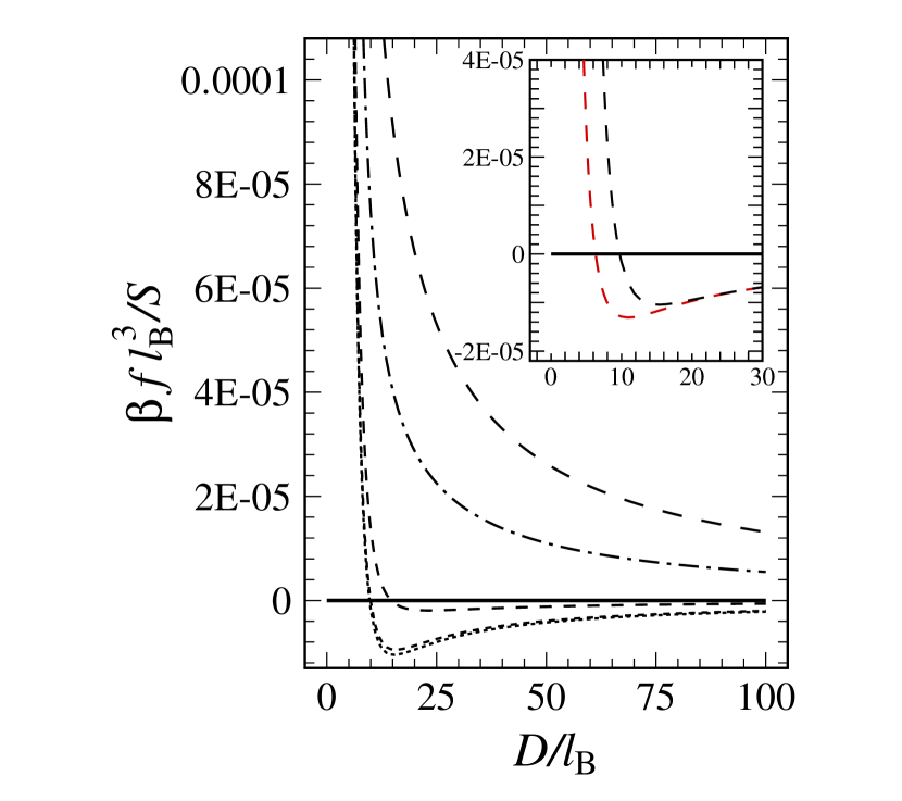
(a)

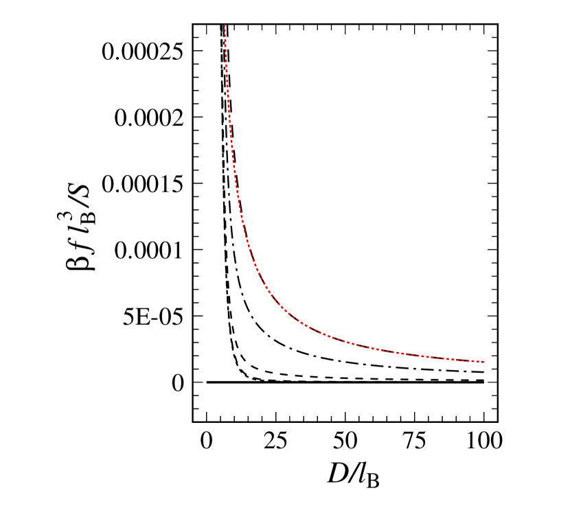
(b)

Figure 3: (Color online) (a) The rescaled total force, $\beta fl_{\mathrm{B}}^{3}/S$, between two dissimilar net-neutral slabs when the dielectric response functions satisfy the relationship $\epsilon_{1}(\imath\xi)<\epsilon_{m}(\imath\xi)<\epsilon_{2}(\imath\xi)$ with the static dielectric constant values $\varepsilon_{1}=5$, $\varepsilon_{m}=10$ and $\varepsilon_{2}=50$. Here we assume $g_{1}=g_{2}=5\times 10^{-8}\,{\mathrm{nm}}^{-3}$ and change $g_{m}=10^{-6},5\times 10^{-7},10^{-7},10^{-8},10^{-10}\,{\mathrm{nm}}^{-3}$ (from top to bottom). The red curve shows the results for $g_{m}=0$ and includes only the zero-frequency contribution in the Lifshitz formula. Inset shows a closer view of the region around the minimum for this latter case (the point of zero force is shifted from $D_{0}\simeq 6.3l_{\mathrm{B}}\simeq 358$ nm, red curve, to $D_{0}\simeq 9.7l_{\mathrm{B}}\simeq 551$ nm, black curve). (b) Same as (a) but for $g_{1}=g_{2}=0$.

In the case where the dielectric response functions of the side slabs are smaller than that of the intervening slab $\epsilon_{1}(\imath\xi),\epsilon_{2}(\imath\xi)<\epsilon_{m}(\imath\xi)$, one encounters a situation which is opposite to the above case, i.e., the pure Casimir-vdW force is attractive vdWgeneral but the disorder force is always repulsive and, as expected, dominates at sufficiently large separations jcp2010 , resulting again in a non-monotonic behavior for the total interaction force between the slabs with a maximum repulsive force at sufficiently high disorder variances as seen in Fig. 2c. In this case, the separation distance $D_{0}$ where the total force vanishes represents an unstable equilibrium distance. In other words, the disorder-induced forces in this case not only oppose the Casimir-vdW force but can also give rise to a potential barrier in the total interaction free energy. Interestingly, in this case the location of the equilibrium moves to larger values of the spacing as well (e.g., from $D_{0}\simeq 1.7l_{\mathrm{B}}\simeq 96.6$ nm to $D_{0}\simeq 2.8l_{\mathrm{B}}\simeq 159.0$ nm for $g_{1}=g_{2}=10^{-6}$ nm^-2 and the parameter values specified in Fig. 2c, inset). This is directly due to the fact that the inclusion of higher-order Matsubara frequencies leads to a larger attractive Casimir-vdW force.

III.2 Role of charge disorder in the intervening medium

So far we focused only on cases where the intervening slab does not contain any disorder charges and examined the role of higher-order Matsubara frequencies. We now proceed by examining the effects that may arise from the presence of charge disorder in the intervening slab, i.e., $g_{m}>0$, and compare the results with those we found in the previous Sections and with the zero-frequency results published elsewhere jcp2010 , where such effects were not included.

Let us first consider the case where the dielectric response functions fulfill the relationship $\epsilon_{1}(\imath\xi)<\epsilon_{m}(\imath\xi)<\epsilon_{2}(\imath\xi)$. This situation was analyzed in Fig. 2b when there is no quenched random charge in intervening slab, i.e., $g_{m}=0$. We now increase the value of $g_{m}$ from $10^{-10}$ up to $10^{-6}$ nm^-3, while keeping $g_{1}=g_{2}=5\times 10^{-8}$ nm^-3 fixed. As seen in Fig. 3a, the non-monotonicity of the interaction profile fades away as the disorder variance in the intervening slab is increased and the interaction between the two semi-infinite slabs becomes strongly repulsive. This also means that the stable bound-state separation $D_{0}$ increases and eventually tends to infinity. It is easy to see that this situation arises because adding further charges in the intervening slab is energetically unfavorable, although the slab remains charge neutral on the average. In order to demonstrate this effect, we set the disorder variance in the two semi-infinite slabs equal to zero, $g_{1}=g_{2}=0$. The total force in this case is repulsive and increases with $g_{m}$, Fig. 3b. In fact, one can easily show that for the case with $g_{1}=g_{2}=0$, the disorder-induced force follows from Eqs. (12) and (28) as

$$\frac{\beta f_{\mathrm{dis}}}{S}=\frac{g_{m}l_{\mathrm{B}}\eta}{2\varepsilon_{m}D},$$ (30)

where

$$\eta=\frac{\varepsilon_{1}\varepsilon_{2}-\varepsilon_{m}^{2}}{(\varepsilon_{1}+\varepsilon_{m})(\varepsilon_{2}+\varepsilon_{m})}.$$ (31)

For the case in Fig. 3b, we have $\eta>0$, and hence the disorder force turns out to be repulsive. In general, when all slabs carry disorder charges and assuming that $g_{1}=g_{2}=g$, we find

$$\frac{\beta f_{\mathrm{dis}}}{S}=\left[-\frac{g\chi}{(\varepsilon_{1}+\varepsilon_{2})}+\frac{g_{m}\eta}{\varepsilon_{m}}\right]\frac{l_{\mathrm{B}}}{2D},$$ (32)

where

$$\chi=\frac{(\varepsilon_{1}-\varepsilon_{m})}{\varepsilon_{2}+\varepsilon_{m}}+\frac{(\varepsilon_{2}-\varepsilon_{m})}{\varepsilon_{1}+\varepsilon_{m}}.$$ (33)

The above formulae clearly show that the disorder-induced force decays quite weakly as $~{}D^{-1}$.

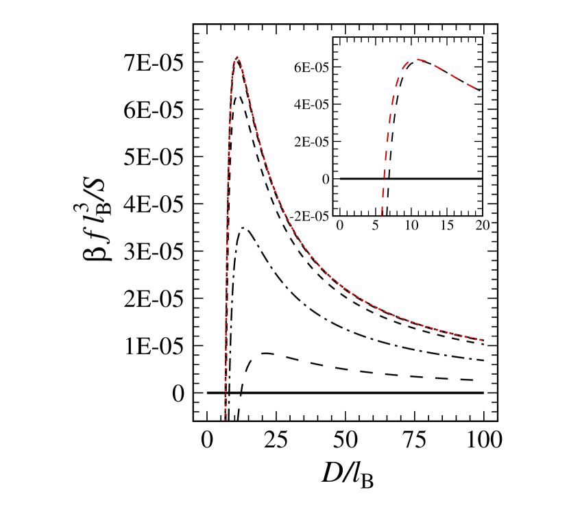
(a)

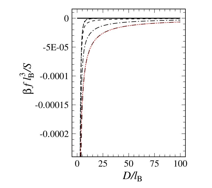
(b)

Figure 4: (Color online) (a) The rescaled total force, $\beta fl_{\mathrm{B}}^{3}/S$, between two dissimilar net-neutral slabs when the dielectric response functions satisfy the relationship $\epsilon_{1}(\imath\xi),\epsilon_{2}(\imath\xi)<\epsilon_{m}(\imath\xi)$ with the static dielectric constant values $\varepsilon_{1}=\varepsilon_{2}=3.81$ (appropriate for SiO₂) and $\varepsilon_{m}=100$. Here we assume $g_{1}=g_{2}=5\times 10^{-8}\,{\mathrm{nm}}^{-3}$ and change $g_{m}=10^{-6},5\times 10^{-7},10^{-7},10^{-8},10^{-10}\,{\mathrm{nm}}^{-3}$ (from bottom to top). The red curve shows the results for $g_{m}=0$ and includes only the zero-frequency contribution in the Lifshitz formula. Inset shows a closer view of the region around the minimum for $g_{m}=10^{-7}\,{\mathrm{nm}}^{-3}$ along with the corresponding zero-frequency results (red curve). (b) Same as (a) but for $g_{1}=g_{2}=0$ and $\varepsilon_{1}=15$, $\varepsilon_{m}=30$ and $\varepsilon_{2}=25$. The red curve shows the corresponding zero-frequency results for $g_{m}=10^{-6}\,{\mathrm{nm}}^{-3}$.

In the case where the dielectric response functions of the bounding slabs are smaller than that of the intervening slabs $\epsilon_{1}(\imath\xi),\epsilon_{2}(\imath\xi)<\epsilon_{m}(\imath\xi)$, introducing quenched disorder charges in the intervening slab suppresses the maximal repulsive force and shifts the point of zero force $D_{0}$ to larger separations as shown in Fig. 4a and the inset. Intuitively, this is because the dielectric images for the charges in the intervening slab are of opposite sign and thus generate attractions when $\varepsilon_{1},\varepsilon_{2}<\varepsilon_{m}$. Equation (30) and the results in Fig. 4b for $g_{1}=g_{2}=0$ clearly demonstrates this effect as we have $\eta<0$ and the only disorder charge contribution comes from those in the intervening slab.

The above results strongly depend on the dielectric difference between the slabs. In fact, the disorder-induced force, Eq. (30), shows a non-monotonic dependence on $\varepsilon_{m}$. If we assume $\varepsilon_{1}=\varepsilon_{2}=\varepsilon<\varepsilon_{m}$, the attractive disorder force will increases in magnitude with $\varepsilon_{m}$ when $\varepsilon_{m}<(1+\sqrt{2})\varepsilon$ and deceases in magnitude otherwise. For instance, in Fig. 5, we choose two identical slabs with $\varepsilon_{1}=\varepsilon_{2}=3.81$ but change the static dielectric constant of the intervening slab from $\varepsilon_{m}=30$ up to 100. The total force becomes increasingly more repulsive and the distance at which the force becomes zero, $D_{0}$, decreases significantly as $\varepsilon_{m}$ is increased as shown in the inset of Fig. 5 (black dots). It should be noted however that the zero-force separation is much larger than what is expected from a zero-frequency calculation jcp2010 , which varies only weakly with $\varepsilon_{m}$ (inset, red dots).

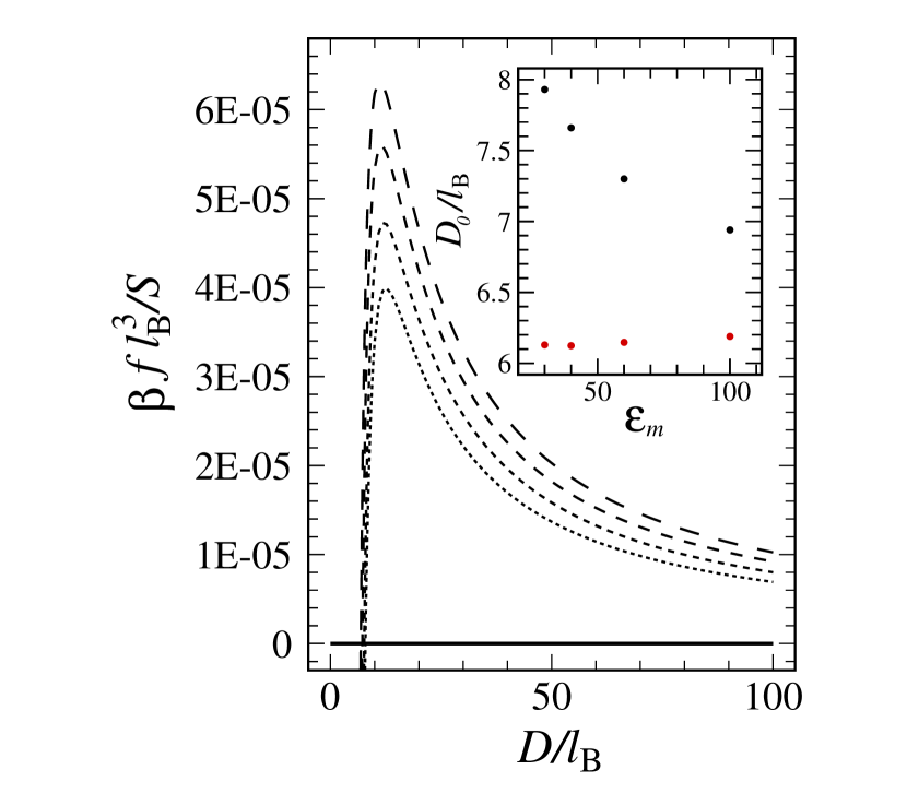
Figure 5: (Color online) The rescaled total force, $\beta fl_{\mathrm{B}}^{3}/S$, between two net-neutral slabs when the dielectric response functions satisfy the relationship $\epsilon_{1}(\imath\xi),\epsilon_{2}(\imath\xi)<\epsilon_{m}(\imath\xi)$ with the static dielectric constant values $\varepsilon_{1}=\varepsilon_{2}=3.81$ (appropriate for SiO₂) and $\varepsilon_{m}=30,40,60$ and 100 (from bottom to top). Here we assume $g_{1}=g_{2}=5\times 10^{-8}\,{\mathrm{nm}}^{-3}$ and $g_{m}=10^{-7}\,{\mathrm{nm}}^{-3}$. Inset shows the location of the zero-force point, $D_{0}$, as a function of $\varepsilon_{m}$ (black dots) compared with the data when only the zero-frequency contribution is included in the Lifshitz formula (red dots).

IV Conclusion

We have studied interactions between randomly charged but otherwise net-neutral slabs by including first, the full spectrum of electromagnetic field fluctuations and second, by taking into account the presence of random charges in the medium between the two slabs. This is done by employing the Lifshitz theory which includes a summation over all Matsubara frequencies, leading to a direct generalization of our previous results prl2010 ; jcp2010 , which were obtained based only on the zero-frequency effects and were thus valid at large separations. This is a crucial new aspect of our analysis of charge disorder as it extends the regime of validity of some of the key findings to the full range of inter-slab separations, especially, down to the nano scale (as long as the continuum model assumed within the Lifshitz theory remains valid).

We can thus draw certain important conclusions regarding the role of disorder effects. In particular, it is shown that the characteristic $\sim D^{-1}$ behavior due to quenched disorder prl2010 sets in well within the retarded regime (e.g., around 50-500 nm in Fig. 2a) and thus the force curves deviate rapidly from the standard (retarded) $\sim D^{-4}$ Casimir-vdW behavior even for highly clean samples with disorder variances down to $10^{-9}\,{\mathrm{nm}}^{-3}$. This behavior should be contrasted with the zero-frequency theory jcp2010 which predicts that the $\sim D^{-1}$ emerges due to a crossover from the classical $\sim D^{-3}$ behavior.

Another remarkable prediction that follows from our present analysis is that the non-monotonic behavior of the total force as a function of distance persists when higher-order Matsubara frequencies are included; however, in almost all cases, the (stable or unstable) equilibrium separation is shifted to much larger values than predicted based solely on the zero-frequency theory jcp2010 . This is important in that it predicts that the disorder-generated non-monotonic behavior of the force is more easily amenable to experimental measurements that expected from zero-frequency calculations.

We have also shown that the presence of charge disorder in the intervening medium leads to another additive contribution to the total force that can be repulsive or attractive depending on the system parameters (such as the relationship between dielectric response functions of the media) and can, for instance, wash out the non-monotonic behavior of the total force. Such non-monotonic behaviors for the interaction between dielectric slabs have received a lot of attention in the context of the Casimir effect and are known to emerge, e.g., in the case of metamaterials metamat and/or other exotic materials such as topological insulators topol , as well as in certain non-trivial geometries geom_casimir ; sernelius . In our analysis the $\sim D^{-1}$ behavior of the force for identical slabs and the non-monotonic force profile for dissimilar slabs represent characteristic fingerprints of the charge disorder and can thus be useful in assessing whether the experimentally observed interactions in ordinary dielectrics can be interpreted in terms of disorder effects.

We presented our results explicitly for the case where the disorder distribution is statistically homogeneous and uncorrelated in space, although the formalism in Section II is in general applicable to layered materials exhibiting finite lateral correlations for the disorder charges as well. Thus, it would be interesting in the future to examine the above-mentioned effects in the situation where the disorder distribution consists of random patches (domains) of finite size jcp2010 , and specifically, when the layering assumption is relaxed and the correlation domains within the slabs have a three-dimensional structure.

V Acknowledgments

A.N. is supported by a Newton International Fellowship from the Royal Society, the Royal Academy of Engineering, and the British Academy. R.P. acknowledges support from ARRS through the program P1-0055 and the research project J1-0908.

References

- (1) Y. Kantor, H. Li and M. Kardar, Phys. Rev. Lett. 69, 61 (1992); I. Borukhov, D. Andelman and H. Orland, Eur. Phys. J. B 5, 869 (1998).
- (2) E. Bianchi, R. Blaak and C.N. Likos, Phys. Chem. Chem. Phys. 13, 6397 (2011).
- (3) E.J.W. Verwey and J.Th.G. Overbeek, Theory of the Stability of Lyophobic Colloids (Elsevier, Amsterdam, 1948); J.N. Israelachvili, Intermolecular and Surface Forces (Academic Press, London, 1990).
- (4) M. Doi and S.F. Edwards, The Theory of Polymer Dynamics (Oxford University Press, New York, 1988).
- (5) D.B. Lukatsky, K.B. Zeldovich and E.I. Shakhnovich, Phys. Rev. Lett. 97 178101 (2006); D.B. Lukatsky and E.I. Shakhnovich, Phys. Rev. E 77, 020901(R) (2008).
- (6) E.E. Meyer, Q. Lin, T. Hassenkam, E. Oroudjev and J.N. Israelachvili, Proc. Natl. Acad. Sci. USA 102, 6839 (2005); S. Perkin, N. Kampf and J. Klein, Phys. Rev. Lett. 96, 038301 (2006); J. Phys. Chem. B 109, 3832 (2005); E.E. Meyer, K.J. Rosenberg and J. Israelachvili, Proc. Natl. Acad. Sci. USA 103, 15739 (2006).
- (7) G. Silbert, D. Ben-Yaakov, Y. Dror, S. Perkin, N. Kampf and J. Klein, e-print: arXiv:1109.4715; See also D. Ben-Yaakov, D. Andelman and H. Diamant, e-print: arXiv:1205.2855.
- (8) H.T. Baytekin, A.Z. Patashinski, M. Branicki, B. Baytekin, S. Soh and B.A. Grzybowski, Science 333, 308 (2011).
- (9) L.F. Zagonel, N. Barrett, O. Renault, A. Bailly, M. Bäurer, M. Hoffmann, S.-J. Shih and D. Cockayne, Surf. Interface Anal. 40, 1709 (2008).
- (10) C.C. Speake and C. Trenkel, Phys. Rev. Lett. 90, 160403 (2003).
- (11) W.J. Kim, M. Brown-Hayes, D.A.R. Dalvit, J.H. Brownell and R. Onofrio, Phys. Rev. A 78, 020101(R) (2008); 79, 026102 (2009); R.S. Decca, E. Fischbach, G.L. Klimchitskaya, D.E. Krause, D. López, U. Mohideen and V.M. Mostepanenko, Phys. Rev. A 79, 026101 (2009); S. de Man, K. Heeck and D. Iannuzzi, Phys. Rev. A 79, 024102 (2009).
- (12) W.J. Kim, A.O. Sushkov, D.A.R. Dalvit and S.K. Lamoreaux, Phys. Rev. Lett. 103, 060401 (2009).
- (13) W.J. Kim, A.O. Sushkov, D.A.R. Dalvit and S.K. Lamoreaux, Phys. Rev. A 81, 022505 (2010).
- (14) W.J. Kim and U.D. Schwarz, J. Vac. Sci. Technol. B 28, C4A1 (2010).
- (15) D. Garcia-Sanchez, K.Y. Fong, H. Bhaskaran, S. Lamoreaux and H.X. Tang, Phys. Rev. Lett. 109, 027202 (2012).
- (16) R. Podgornik and A. Naji, Europhys. Lett. 74, 712 (2006).
- (17) A. Naji, D.S. Dean, J. Sarabadani, R.R. Horgan and R. Podgornik, Phys. Rev. Lett. 104, 060601 (2010).
- (18) J. Sarabadani, A. Naji, D.S. Dean, R.R. Horgan and R. Podgornik, J. Chem. Phys. 133, 174702 (2010).
- (19) D.S. Dean, A. Naji and R. Podgornik, Phys. Rev. E 83, 011102 (2011).
- (20) A. Naji, J. Sarabadani, D.S. Dean and R. Podgornik, Eur. Phys. J. E 35, 24 (2012).
- (21) V.A. Parsegian, Van der Waals Forces (Cambridge University Press, Cambridge, 2005).
- (22) J. Mahanty and B.W. Ninham, Dispersion Forces (Academic Press, London, 1976).
- (23) J. Sarabadani and M. F. Miri, Phys. Rev. A 84, 032503 (2011).
- (24) See, e.g., F.S.S. Rosa, D.A.R. Dalvit and P.W. Milonni, Phys. Rev. Lett. 100, 183602 (2008); A.W. Rodriguez, J.D. Joannopoulos and S.G. Johnson, Phys. Rev. A 77, 062107 (2008); R. Zhao, J. Zhou, Th. Koschny, E.N. Economou and C.M. Soukoulis, Phys. Rev. Lett. 103, 103602 (2009).
- (25) A.G. Grushin and A. Cortijo, Phys. Rev. Lett. 106, 020403 (2011).
- (26) M. Levin, A.P. McCauley, A.W. Rodriguez, M.T. Homer Reid and S.G. Johnson, Phys. Rev. Lett. 105, 090403 (2010); K.A. Milton, E.K. Abalo, P. Parashar, N. Pourtolami, I. Brevik and S.Å. Ellingsen, Phys. Rev. A 83, 062507 (2011); M.F. Maghrebi, Phys. Rev. D 83, 045004 (2011).
- (27) M. Boström, B.W. Ninham, I. Brevik, C. Persson, D.F. Parsons and B.E. Sernelius, Appl. Phys. Lett. 100, 253104 (2012).
- (28) The generalization to the case where bounding surfaces may also carry a disordered surface charge density is straightforward and has been discussed in previous works epl2006 ; prl2010 ; jcp2010 ; pre2011 ; epje2012 but will not be considered in the present work.
- (29) D.S. Dean, R.R. Horgan, A. Naji and R. Podgornik, Phys. Rev. A 79, 040101(R) (2009).
- (30) D.S. Dean, R.R. Horgan, A. Naji and R. Podgornik, Phys. Rev. E 81, 051117 (2010).
- (31) A. Naji and R. Podgornik, Phys. Rev. E 72, 041402 (2005).
- (32) Y.S. Mamasakhlisov, A. Naji and R. Podgornik, J. Stat. Phys. 133, 659 (2008).
- (33) F. Wooten, Optical Properties of Solids (Academic Press, New York, 1972).
- (34) D.B. Hough and L.R. White, Adv. Colloid Interface Sci. 14, 3 (1980).
- (35) K.C. Kao, Dielectric Phenomena in Solids (Elsevier Academic Press, San Diego, 2004); L.P. Pitaevskii, Phys. Rev. Lett. 101, 163202 (2008).
- (36) J.N. Munday, F. Capasso and V.A. Parsegian, Nature 457, 170 (2009)
- (37) M. Boström, S.Å. Ellingsen, I. Brevik, D.F. Parsons and B.E. Sernelius, Phys. Rev. A 85, 064501 (2012).