Differentially Private Kalman Filtering

Abstract

This paper studies the $\mathcal{H}_{2}$ (Kalman) filtering problem in the situation where a signal estimate must be constructed based on inputs from individual participants, whose data must remain private. This problem arises in emerging applications such as smart grids or intelligent transportation systems, where users continuously send data to third-party aggregators performing global monitoring or control tasks, and require guarantees that this data cannot be used to infer additional personal information. To provide strong formal privacy guarantees against adversaries with arbitrary side information, we rely on the notion of differential privacy introduced relatively recently in the database literature. This notion is extended to dynamic systems with many participants contributing independent input signals, and mechanisms are then proposed to solve the $\mathcal{H}_{2}$ filtering problem with a differential privacy constraint. A method for mitigating the impact of the privacy-inducing mechanism on the estimation performance is described, which relies on controlling the $\mathcal{H}_{\infty}$ norm of the filter. Finally, we discuss an application to a privacy-preserving traffic monitoring system.

I Introduction

In many applications, such as smart grids, population health monitoring, or traffic monitoring, the efficiency of the system relies on the participation of the users to provide reliable data in real-time, e.g., power consumption, sickness symptoms, or GPS coordinates. However, for privacy or security reasons, the participants benefiting from these services generally do not want to release more information than strictly necessary. Unfortunately, examples of unintended loss of privacy already abound. Indeed, it is possible to infer from the trace of a smart meter the type of appliances present in a house as well as the occupants’ daily activities [1], to re-identify an anonymous GPS trace by correlating it with publicly available information such as location of work [2], or to infer individual transactions on commercial websites from temporal changes in public recommendation systems [3]. Providing rigorous guarantees to the users about the privacy risks incurred is thus crucial to encourage participation and ultimately realize the benefits promised by these systems.

In our recent work [4], we introduced privacy concerns in the the context of systems theory, by relying on the notion of differential privacy [5], a particularly successful definition of privacy used in the database literature. This notion is motivated by the fact that any useful information provided by a dataset about a group of people can compromise the privacy of specific individuals due to the existence of side information. Differentially private mechanisms randomize their responses to dataset analysis requests and guarantee that whether or not an individual chooses to contribute her data only marginally changes the distribution over the published outputs. As a result, even an adversary cross-correlating these outputs with other sources of information cannot infer much more about specific individuals after publication than before [6].

Most work related to privacy is concerned with the analysis of static databases, whereas cyber-physical systems clearly emphasize the need for mechanisms working with dynamic, time-varying data streams. Recently, information-theoretic approaches have been proposed to guarantee some level of privacy when releasing time series [7, 8]. However, the resulting privacy guarantees only hold if the statistics of the participants’ data streams obey the assumptions made (typically stationarity, dependence and distributional assumptions), and require the explicit statistical modeling of all available side information. This task is impossible in general as new, as-yet-unknown side information can become available after releasing the results. In contrast, differential privacy is a worst-case notion that holds independently of any probabilistic assumption on the dataset, and controls the information leakage against adversaries with arbitrary side information [6]. Once such a privacy guarantee is enforced, one can still leverage potential additional statistical information about the dataset to improve the quality of the outputs.

In this paper, we pursue our work on differential privacy for dynamical systems [4], by considering the $\mathcal{H}_{2}$ filtering problem (or steady-state Kalman filtering) with a differential privacy constraint. In this problem, the goal is to minimize an estimation error variance for a desired linear combination of the participants’ state trajectories, based on their contributed measurements, while guaranteeing the privacy of the individual signals. In contrast to the generic filtering mechanisms presented in [4], we emphasize here how a model of the participants’ dynamics can be leveraged to publish more accurate results, without compromising the differential privacy guarantee if this model is not accurate. Section II provides some technical background on differential privacy and Section III describes a basic mechanism enforcing privacy for dynamical systems by injecting additional white noise. As shown in [4], accurate private results can be published for filters with small incremental gains with respect to the individual input channels. This leads us in Section IV to present a modification of the standard Kalman filter, essentially controlling its $\mathcal{H}_{\infty}$ norm simultaneously with the steady-state estimation error, in order to minimize the impact of the privacy-inducing mechanism. Finally, Section V describes an application to a simplified traffic monitoring system relying on location traces from the participants to provide an average velocity estimate on a road segment. Most proofs are omitted from this extended abstract and will appear in the full version of the paper.

II Differential Privacy

In this section we review the notion of differential privacy [5] as well as a basic mechanism that can be used to achieve it when the released data belongs to a finite-dimensional vector space. We refer the reader to the surveys by Dwork, e.g., [9], for additional background on differential privacy.

II-A Definition

Let us fix some probability space $(\Omega,\mathcal{F},\mathbb{P})$. Let $\mathsf{D}$ be a space of datasets of interest (e.g., a space of data tables, or a signal space). A mechanism is just a map $M:\mathsf{D}\times\Omega\to\mathsf{R}$, for some measurable output space $\mathsf{R}$, such that for any element $d\in\mathsf{D}$, $M(d,\cdot)$ is a random variable, typically writen simply $M(d)$. A mechanism can be viewed as a probabilistic algorithm to answer a query $q$, which is a map $q:\mathsf{D}\to\mathsf{R}$. In some cases, we index the mechanism by the query $q$ of interest, writing $M_{q}$.

Example II.1

Let $\mathsf{D}=\mathbb{R}^{n}$, with each real-valued entry of $d\in\mathsf{D}$ corresponding to some sensitive information for an individual contributing her data. A data analyst would like to know the average of the entries of $d$, i.e., her query is

$$q:\mathsf{D}\to\mathbb{R},\;\;q(d)=\frac{1}{n}\sum_{i=1}^{n}d_{i}.$$

As detailed in Section II-B, a typical mechanism $M_{q}$ to answer this query in a differentially private way computes $q(d)$ and blurs the result by adding a random variable $Y:\Omega\to\mathbb{R}$

$$M_{q}:\mathsf{D}\times\Omega\to\mathbb{R},\;\;M_{q}(d)=\frac{1}{n}\sum_{i=1}^{n}d_{i}+Y.$$

Note that in the absence of perturbation $Y$, an adversary who knows $n$ and $d_{j},j\geq 2,$ can recover the remaining entry $d_{1}$ exactly if he learns $q(d)$. This can deter people from contributing their data, even though broader participation improves the accuracy of the analysis and thus can be beneficial to the population as a whole.

Next, we introduce the definition of differential privacy. We call a measure $\mu$ on $\mathsf{R}$ $\delta$-bounded if it is a finite positive measure with $\mu(\mathsf{R})\leq\delta$. Intuitively in the following definition, $\mathsf{D}$ is a space of datasets of interest, and we have a binary relation Adj on $\mathsf{D}$, called adjacency, such that $\text{Adj}(d,d^{\prime})$ if and only if $d$ and $d^{\prime}$ differ by the data of a single participant.

Definition 1

Let $\mathsf{D}$ be a space equipped with a binary relation denoted Adj, and let $(\mathsf{R},\mathcal{M})$ be a measurable space. Let $\epsilon,\delta\geq 0$. A mechanism $M:\mathsf{D}\times\Omega\to\mathsf{R}$ is $(\epsilon,\delta)$-differentially private if there exists a $\delta$-bounded measure $\mu$ on $(\mathsf{R},\mathcal{M})$ such that for all $d,d^{\prime}\in\mathsf{D}$ such that $\text{Adj}(d,d^{\prime})$ and for all $S\in\mathcal{M}$, we have

$$\mathbb{P}(M(d)\in S)\leq e^{\epsilon}\mathbb{P}(M(d^{\prime})\in S)+\mu(S).$$ (1)

If $\delta=0$, the mechanism is said to be $\epsilon$-differentially private.

This definition is essentially the same as the one introduced in [5] and subsequent work, except for the fact that $\mu(S)$ in (1) is usually replaced by the constant $\delta$. The definition says that for two adjacent datasets, the distributions over the outputs of the mechanism should be close. The choice of the parameters $\epsilon,\delta$ is set by the privacy policy. Typically $\epsilon$ is taken to be a small constant, e.g., $\epsilon\approx 0.1$ or perhaps even $\ln 2$ or $\ln 3$. The parameter $\delta$ should be kept small as it controls the probability of certain significant losses of privacy, e.g., when a zero probability event for input $d^{\prime}$ becomes an event with positive probability for input $d$ in (1).

Remark 1

The definition of differential privacy depends on the choice of $\sigma$-algebra $\mathcal{M}$ in Definition 1. When we need to state this $\sigma$-algebra explicitly, we write $M:\mathsf{D}\times\Omega\to(\mathsf{R},\mathcal{M})$. In particular, this $\sigma$-algebra should be sufficiently “rich”, since (1) is trivially satisfied by any mechanism if $\mathcal{M}=\{\emptyset,\mathsf{R}\}$.

A useful property of the notion of differential privacy is that no additional privacy loss can occur by simply manipulating an output that is differentially private. This result is similar in spirit to the data processing inequality from information theory [10].

Theorem 1 (resilience to post-processing)

Let $M_{1}:\mathsf{D}\times\Omega\to(\mathsf{R}_{1},\mathcal{M}_{1})$ be an $(\epsilon,\delta)$-differentially private mechanism. Let $M_{2}:\mathsf{D}\times\Omega\to(\mathsf{R}_{2},\mathcal{M}_{2})$ be another mechanism such that for all $S\in\mathcal{M}_{2}$, there exists a nonnegative measurable function $f_{S}$ such that for all $d\in\mathsf{D}$, we have

$$\mathbb{P}(M_{2}(d)\in S|M_{1}(d))=f_{S}(M_{1}(d)),\forall d\in\mathsf{D}.$$ (2)

Then $M_{2}$ is $(\epsilon,\delta)$-differentially private.

Remark 1

Suppose that $M_{1}$ takes its values in a discrete set. Then the condition (2) says that the conditional distribution $\mathbb{P}(M_{2}(d)\in S|M_{1}(d)=m_{1})$ for a given element $m_{1}$ does not further depend of $d$. In other words, a mechanism $M_{2}$ accessing the dataset only indirectly via the output of $M_{1}$ cannot weaken the privacy guarantee. Hence post-processing can be used to improve the accuracy of an output, without weakening the privacy guarantee.

II-B A Basic Differentially Private Mechanism

A mechanism that throws away all the information in a dataset is obviously private, but not useful, and in general one has to trade off privacy for utility when answering specific queries. We recall below a basic mechanism that can be used to answer queries in a differentially private way. We are only concerned in this section with queries that return numerical answers, i.e., here a query is a map $q:\mathsf{D}\to\mathsf{R}$, where the output space $\mathsf{R}$ equals $\mathbb{R}^{k}$ for some $k>0$, is equipped with a norm denoted $\|\cdot\|_{\mathsf{R}}$, and the $\sigma$-algebra $\mathcal{M}$ on $\mathsf{R}$ is taken to be the standard Borel $\sigma$-algebra, denoted $\mathcal{R}^{k}$. The following quantity plays an important role in the design of differentially private mechanisms [5].

Definition 2

Let $\mathsf{D}$ be a space equipped with an adjacency relation Adj. The sensitivity of a query $q:\mathsf{D}\to\mathsf{R}$ is defined as

$$\Delta_{\mathsf{R}}q:=\max_{d,d^{\prime}:\text{Adj}(d,d^{\prime})}\|q(d)-q(d^{\prime})\|_{\mathsf{R}}.$$

In particular, for $\mathsf{R}=\mathbb{R}^{k}$ equipped with the $p$-norm $\|x\|_{p}=\left(\sum_{i=1}^{k}|x_{i}|^{p}\right)^{1/p}$, for $p\in[1,\infty]$, we denote the $\ell_{p}$ sensitivity by $\Delta_{p}q$.

A differentially private mechanism proposed in [11], modifies an answer to a numerical query by adding iid zero-mean noise distributed according to a Gaussian distribution. Recall the definition of the $\mathcal{Q}$-function

$$\mathcal{Q}(x):=\frac{1}{\sqrt{2\pi}}\int_{x}^{\infty}e^{-\frac{u^{2}}{2}}du.$$

The following theorem tightens the analysis from [11].

Theorem 2

Let $q:\mathsf{D}\to\mathbb{R}^{k}$ be a query. Then the Gaussian mechanism $M_{Q}:\mathsf{D}\times\Omega\to\mathbb{R}^{k}$ defined by $M_{q}(d)=q(d)+w$, with $w\sim\mathcal{N}\left(0,\sigma^{2}I_{k}\right)$, where $\sigma\geq\frac{\Delta_{2}q}{2\epsilon}(K+\sqrt{K^{2}+2\epsilon})$ and $K=\mathcal{Q}^{-1}(\delta)$, is $(\epsilon,\delta)$-differentially private.

For the rest of the paper, we define

$$\kappa(\delta,\epsilon)=\frac{1}{2\epsilon}(K+\sqrt{K^{2}+2\epsilon}),$$

so that the standard deviation $\sigma$ in Theorem 2 can be written $\sigma(\delta,\epsilon)=\kappa(\epsilon,\delta)\Delta_{2}q$. It can be shown that $\kappa(\delta,\epsilon)$ behaves roughly as $O(\ln(1/\delta))^{1/2}/\epsilon$. For example, to guarantee $(\epsilon,\delta)$-differential privacy with $\epsilon=\ln(2)$ and $\delta=0.05$, we obtain that the standard deviation of the Gaussian noise introduced should be about $2.65$ times the $\ell_{2}$-sensitivity of $q$.

III Differentially Private Dynamic Systems

In this section we review the notion of differential privacy for dynamic systems, following [4]. We start with some notations and technical prerequisites. All signals are discrete-time signals and all systems are assumed to be causal. For each time $T$, let $P_{T}$ be the truncation operator, so that for any signal $x$ we have

$$(P_{T}x)_{t}=\begin{cases}x_{t},&t\leq T\\ 0,&t>T.\end{cases}$$

Hence a deterministic system $\mathcal{G}$ is causal if and only if $P_{T}\mathcal{G}=P_{T}\mathcal{G}P_{T}$. We denote by $\ell_{p,e}^{m}$ the space of sequences with values in $\mathbb{R}^{m}$ and such that $x\in\ell_{p,e}^{m}$ if and only if $P_{T}x$ has finite $p$-norm for all integers $T$. The $\mathcal{H}_{2}$ norm and $\mathcal{H}_{\infty}$ norm of a stable transfer function $\mathcal{G}$ are defined respectively as

$$\|\mathcal{G}\|_{2} =\left(\frac{1}{2\pi}\int_{-\pi}^{\pi}\text{Tr}(\mathcal{G}^{*}(e^{i\omega})\mathcal{G}(e^{i\omega}))d\omega\right)^{1/2},$$

$$\|\mathcal{G}\|_{\infty} =\text{ess}\sup_{\omega\in[-\pi,\pi)}\sigma_{\max}(\mathcal{G}(e^{i\omega})),$$

where $\sigma_{\max}(A)$ denotes the maximum singular value of a matrix $A$.

We consider situations in which private participants contribute input signals driving a dynamic system and the queries consist of output signals of this system. We assume that the input of a system consists of $n$ signals, one for each participant. An input signal is denoted $u=(u_{1},\ldots,u_{n})$, with $u_{i}\in\ell_{r_{i},e}^{m_{i}}$ for some $m_{i}\in\mathbb{N}$ and $r_{i}\in[1,\infty]$. A simple example is that of a dynamic system releasing at each period the average over the past $l$ periods of the sum of the input values of the participants, i.e., with output $\frac{1}{l}\sum_{k=t-l+1}^{t}\sum_{i=1}^{n}u_{i,k}$ at time $t$. For $r=(r_{1},\ldots,r_{n})$ and $m=(m_{1},\ldots,m_{n})$, an adjacency relation can be defined on $l_{r,e}^{m}=\ell_{r_{1},e}^{m_{1}}\times\ldots\times\ell_{r_{n},e}^{m_{n}}$ by $\text{Adj}(u,u^{\prime})$ if and only if $u$ and $u^{\prime}$ differ by exactly one component signal, and moreover this deviation is bounded. That is, let us fix a set of nonnegative numbers $b=(b_{1},\ldots,b_{n})$, $b_{i}\geq 0$, and define

$$\text{Adj}^{b}(u,u^{\prime})\text{ iff for some }i,\|u_{i}-u_{i}^{\prime}\|_{r_{i}}\leq b_{i},$$ (3)

$$\text{and }u_{j}=u_{j}^{\prime}\text{ for all }j\neq i.$$

Note that in (3) two signals $u_{i},u_{i}^{\prime}$ are considered different if there exists some time $t$ at which $u_{i,t}\neq u^{\prime}_{i,t}$.

III-A The Dynamic Gaussian Mechanism

Recall (see, e.g., [12]) that for a system $F$ with inputs in $\ell_{r,e}^{m}$ and output in $\ell_{s,e}^{m^{\prime}}$, its $\ell_{r}$-to-$\ell_{s}$ incremental gain $\gamma^{inc}_{r,s}(F)$ is defined as the smallest number $\gamma$ such that

$$\|P_{T}Fu-P_{T}Fu^{\prime}\|_{s}\leq\gamma\|P_{T}u-P_{T}u^{\prime}\|_{r},\;\;\forall u,u^{\prime}\in\ell_{r,e}^{m},$$

for all $T$. Now consider, for $r=(r_{1},\ldots,r_{n})$ and $m=(m_{1},\ldots,m_{n})$, a system $\mathcal{G}$ defined by

$$\mathcal{G}:l^{m}_{r,e}\to\ell_{s,e}^{m^{\prime}}$$

$$\mathcal{G}(u_{1},\ldots,u_{n})=\sum_{i=1}^{n}\mathcal{G}_{i}u_{i},$$ (4)

where $\mathcal{G}_{i}:\ell_{r_{i},e}^{m_{i}}\to\ell_{s,e}^{m^{\prime}}$, for all $1\leq i\leq n$.

Theorem 3

Let $\mathcal{G}$ be defined as in (4) and consider the adjacency relation (3). Then the mechanism $Mu=\mathcal{G}u+w$, where $w$ is a white noise with $w_{t}\sim\mathcal{N}(0,\sigma^{2}I_{m^{\prime}})$ and $\sigma\geq\kappa(\delta,\epsilon)\max_{1\leq i\leq n}\{\gamma^{inc}_{r_{i},2}(\mathcal{G}_{i})\,b_{i}\}$, is $(\epsilon,\delta)$-differentially private.

Corollary 1

Let $\mathcal{G}$ be defined as in (4) with each system $\mathcal{G}_{i}$ linear, and $r_{i}=2$ for all $1\leq i\leq n$. Then the mechanism $Mu=\mathcal{G}u+w$, where $w$ is a white Gaussian noise with $w_{t}\sim\mathcal{N}(0,\sigma^{2}I_{m^{\prime}})$ and $\sigma\geq\kappa(\delta,\epsilon)\max_{1\leq i\leq n}\{\|\mathcal{G}_{i}\|_{\infty}\,b_{i}\}$, is $(\epsilon,\delta)$-differentially private for (3).

III-B Filter Approximation Set-ups for Differential Privacy

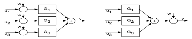
Figure 1: Two architectures for differential privacy. (a) Input perturbation. (b) Output perturbation.

Let $r_{i}=2$ for all $i$ and $\mathcal{G}$ be linear as in the Corollary 1, and assume for simplicity the same bound $b_{1}^{2}=\ldots=b_{n}^{2}=\mathcal{E}$ for the allowed variations in energy of each input signal. We have then two simple mechanisms producing a differentially private version of $\mathcal{G}$, depicted on Fig. 1. The first one directly perturbs each input signal $u_{i}$ by adding to it a white Gaussian noise $w_{i}$ with $w_{i,t}\sim\mathcal{N}(0,\sigma^{2}I_{m_{i}})$ and $\sigma^{2}=\kappa(\delta,\epsilon)^{2}\mathcal{E}$. These perturbations on each input channel are then passed through $\mathcal{G}$, leading to a mean squared error (MSE) for the output equal to $\kappa(\delta,\epsilon)^{2}\mathcal{E}\|\mathcal{G}\|^{2}_{2}=\kappa(\delta,\epsilon)^{2}\mathcal{E}\sum_{i=1}^{n}\|\mathcal{G}_{i}\|^{2}_{2}$. Alternatively, we can add a single source of noise at the output of $\mathcal{G}$ according to Corollary 1, in which case the MSE is $\kappa(\delta,\epsilon)^{2}\mathcal{E}\max_{1\leq i\leq n}\{\|\mathcal{G}_{i}\|_{\infty}^{2}\}$. Both of these schemes should be evaluated depending on the system $\mathcal{G}$ and the number $n$ of participants, as none of the error bound is better than the other in all circumstances. For example, if $n$ is small or if the bandwidths of the individual transfer functions $\mathcal{G}_{i}$ do not overlap, the error bound for the input perturbation scheme can be smaller. Another advantage of this scheme is that the users can release differentially private signals themselves without relying on a trusted server. However, there are cryptographic means for achieving the output perturbation scheme without centralized trusted server as well, see, e.g., [13].

Example III.1

Consider again the problem of releasing the average over the past $l$ periods of the sum of the input signals, i.e., $\mathcal{G}=\sum_{i=1}^{n}\mathcal{G}_{i}$ with

$$(\mathcal{G}_{i}u_{i})_{t} =\frac{1}{l}\sum_{k=t-l+1}^{t}u_{i,k},$$

for all $i$. Then $\|\mathcal{G}_{i}\|_{2}^{2}=1/l$, whereas $\|\mathcal{G}_{i}\|_{\infty}=1$, for all $i$. The MSE for the scheme with the noise at the input is then $\kappa(\delta,\epsilon)^{2}\mathcal{E}n/l$. With the noise at the output, the MSE is $\kappa(\delta,\epsilon)^{2}\mathcal{E}$, which is better exactly when $n>l$, i.e., the number of users is larger than the averaging window.

IV Kalman Filtering

We now discuss the Kalman filtering problem subject to a differential privacy constraint. With respect to the previous section, for Kalman filtering it is assumed that more is publicly known about the dynamics of the processes producing the individual signals. The goal here is to guarantee differential privacy for the individual state trajectories. Section V describes an application of the differentially private mechanisms presented here to a stylized traffic monitoring problem.

IV-A A Differentially Private Kalman Filter

Consider a set of $n$ linear systems, each with independent dynamics

$$x_{i,t+1}=A_{i}x_{i,t}+B_{i}w_{i,t},\;\;t\geq 0,\;\;1\leq i\leq n,$$ (5)

where $w_{i}$ is a standard zero-mean Gaussian white noise process with covariance $\mathbb{E}[w_{i,t}w_{i,t^{\prime}}]=\delta_{t-t^{\prime}}$, and the initial condition $x_{i,0}$ is a Gaussian random variable with mean $\bar{x}_{i,0}$, independent of the noise process $w_{i}$. System $i$, for $1\leq i\leq n$, sends measurements

$$y_{i,t}=C_{i}x_{i,t}+D_{i}w_{i,t}$$ (6)

to a data aggregator. We assume for simplicity that the matrices $D_{i}$ are full row rank, and that $B_{i}D_{i}^{T}=0$, i.e., the process and measurement noises are uncorrelated.

The data aggregator aims at releasing a signal that asymptotically minimizes the minimum mean squared error with respect to a linear combination of the individual states. That is, the quantity of interest to be estimated at each period is $z_{t}=\sum_{i=1}^{n}L_{i}x_{i,t}$, where $L_{i}$ are given matrices, and we are looking for a causal estimator $\hat{z}$ constructed from the signals $y_{i},1\leq i\leq n$, solution of

$$\min_{\hat{z}}\lim_{T\to\infty}\frac{1}{T}\sum_{t=0}^{T-1}E\left[\|z_{t}-\hat{z}_{t}\|_{2}^{2}\right].$$

The data $\bar{x}_{i,0},A_{i},B_{i},C_{i},D_{i},L_{i},1\leq i\leq n,$ are assumed to be public information. For all $1\leq i\leq n$, we assume that the pairs $(A_{i},C_{i})$ are detectable and the pairs $(A_{i},B_{i})$ are stabilizable. In the absence of privacy constraint, the optimal estimator is $\hat{z}_{t}=\sum_{i=1}^{n}L_{i}\hat{x}_{i,t}$, with $\hat{x}_{i,t}$ provided by the steady-state Kalman filter [14]. Figure 2 shows this initial set-up.

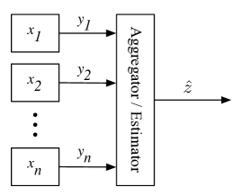
Figure 2: Kalman filtering set-up.

Suppose now that the publicly released estimate $\hat{z}$ should guarantee the differential privacy of the participants. This requires that we first specify an adjacency relation on the appropriate space of datasets. Let $x=[x_{1}^{T},\ldots,x_{n}^{T}]^{T}$ and $y=[y_{1}^{T},\ldots,y_{n}^{T}]^{T}$ denote the global state and measurement signals. Assume that the mechanism is required to guarantee differential privacy with respect to a subset $\mathcal{S}_{i}:=\{i_{1},\ldots,i_{k}\}$ of the coordinates of the state trajectory $x_{i}$. Let the matrix $T_{i}$ be the diagonal matrix with $[T_{i}]_{jj}=1$ if $j\in\mathcal{S}_{i}$, and $[T_{i}]_{jj}=0$ otherwise. Hence $T_{i}v$ sets the coordinates of a vector $v$ which do not belong to the set $\{i_{1},\ldots,i_{k}\}$ to zero. Fix a vector $\rho\in\mathbb{R}_{+}^{n}$. The adjacency relation considered here is

$$\text{Adj}_{\mathcal{S}}^{\rho}(x,x^{\prime})\text{ iff }\text{for some }i,\;\|T_{i}x_{i}-T_{i}x_{i}^{\prime}\|_{2}\leq\rho_{i},$$ (7)

$$(I-T_{i})x_{i}=(I-T_{i})x_{i}^{\prime},\text{and }x_{j}=x_{j}^{\prime}\text{ for all }j\neq i.$$

In words, two adjacent global output signals differ by the trajectory of a single participant, say $i$. Moreover, for differential privacy guarantees we are constraining the range in energy variation in the signal $T_{i}x_{i}$ of participant $i$ to be at most $\rho_{i}^{2}$. Hence, the distribution on the released results should be essentially the same if a participant’s output signal value $T_{i}x_{i,t_{0}}$ at some single specific time $t_{0}$ were replaced by $T_{i}x^{\prime}_{i,t_{0}}$ with $\|T_{i}(x_{i,t_{0}}-x^{\prime}_{i,t_{0}})\|\leq\rho_{i}$, but the privacy guarantee should also hold for smaller instantaneous deviations on longer segments of trajectory.

Depending on which signals on Fig. 2 are actually published, and similarly to the discussion of Section III-B, there are different points at which a privacy inducing noise can be introduced. First, for the input noise injection mechanism, the noise can be added by each participant directly to their transmitted measurement signal $y_{i}$. Namely, since for two state trajectories $x_{i},x_{i}^{\prime}$ adjacent according to (7) we have for the corresponding measured signals

$$\|y_{i}-y_{i}^{\prime}\|_{2}=\|C_{i}T_{i}(x_{i}-x_{i}^{\prime})\|_{2},$$

differential privacy can be guaranteed if participant $i$ adds to $y_{i}$ a white Gaussian noise with covariance matrix $\kappa(\delta,\epsilon)^{2}\rho_{i}^{2}\sigma^{2}_{\max}(C_{i}T_{i})I_{p_{i}}$, where $p_{i}$ is the dimension of $y_{i,t}$. Note that in this sensitivity computation the measurement noise $D_{i}w_{i}$ has the same realization independently of the considered variation in $x_{i}$. At the data aggregator, this additional noise can be taken into account in the design of the Kalman filter, since it can simply be viewed as an additional measurement noise. Again, an important advantage of this mechanism is its simplicity of implementation when the participants do not trust the data aggregator, since the transmitted signals are already differentially private.

Next, consider the output noise injection mechanism. Since we assume that $\bar{x}^{i}_{0}$ is public information, the initial condition $\hat{x}_{i,0}$ of each state estimator is fixed. Consider now two state trajectories $x,x^{\prime}$, adjacent according to (7), and let $\hat{z},\hat{z}^{\prime}$ be the corresponding estimates produced. We have

$$\hat{z}-\hat{z}^{\prime}=L_{i}\mathcal{K}_{i}(y_{i}-y_{i}^{\prime})=L_{i}\mathcal{K}_{i}C_{i}T_{i}(x_{i}-x_{i}^{\prime}),$$

where $\mathcal{K}_{i}$ is the $i^{th}$ Kalman filter. Hence $\|\hat{z}-\hat{z}^{\prime}\|_{2}\leq\gamma_{i}\rho_{i},$ where $\gamma_{i}$ is the $\mathcal{H}_{\infty}$ norm of the transfer function $L_{i}\mathcal{K}_{i}C_{i}T_{i}$. We thus have the following theorem.

Theorem 4

A mechanism releasing $\left(\sum_{i=1}^{n}L_{i}\mathcal{K}_{i}y_{i}\right)+\gamma\kappa(\delta,\epsilon)\;\nu$, where $\nu$ is a standard white Gaussian noise independent of $\{w_{i}\}_{1\leq i\leq n},\{x_{i,0}\}_{1\leq i\leq n}$, and $\gamma=\max_{1\leq i\leq n}\{\gamma_{i}\rho_{i}\}$, with $\gamma_{i}$ the $\mathcal{H}_{\infty}$ norm of $L_{i}\mathcal{K}_{i}C_{i}T_{i}$, is differentially private for the adjacency relation (7).

IV-B Filter Redesign for Stable Systems

In the case of the output perturbation mechanism, one can potentially improve the MSE of the filter with respect to the Kalman filter considered in the previous subsection. Namely, consider the design of $n$ filters of the form

$$\hat{x}_{i,t+1} =F_{i}\hat{x}_{i,t}+G_{i}y_{i,t}$$ (8)

$$\hat{z}_{i,t} =H_{i}\hat{x}_{i,t}+K_{i}y_{i,t},$$ (9)

for $1\leq i\leq n$, where $F_{i},G_{i},H_{i},K_{i}$ are matrices to determine. The estimator considered is

$$\hat{z}_{t}=\sum_{i=1}^{n}\hat{z}_{i,t},$$

so that each filter output $\hat{z}_{i}$ should minimize the steady-state error variance with $z_{i}=L_{i}x_{i}$, and the released signal $\hat{z}$ should guarantee the differential privacy with respect to (7). Assume first in this section that the system matrices $A_{i}$ are stable, in which case we also restrict the filter matrices $F_{i}$ to be stable. Moreover, we only consider the design of full order filters, i.e., the dimensions of $F_{i}$ are greater or equal to those of $A_{i}$, for all $1\leq i\leq n$. Finally, we remove the simplifying assumption $B_{i}D_{i}^{T}=0$.

Denote the overall state for each system and associated filter by $\tilde{x}_{i}=[x_{i}^{T},\hat{x}_{i}^{T}]^{T}$. The combined dynamics from $w_{i}$ to the estimation error $e_{i}:=z_{i}-\hat{z}_{i}$ can then be written

$$\tilde{x}_{i,t+1} =\tilde{A}_{i}\tilde{x}_{i,t}+\tilde{B}_{i}w_{i,t}$$

$$e_{i,t} =\tilde{C}_{i}\tilde{x}_{i,t}+\tilde{D}_{i}w_{i,t},$$

where

$$\tilde{A}_{i} =\begin{bmatrix}A_{i}&0\\ G_{i}C_{i}&F_{i}\end{bmatrix},\;\;\tilde{B}_{i}=\begin{bmatrix}B_{i}\\ G_{i}D_{i}\end{bmatrix},$$

$$\tilde{C}_{i} =\begin{bmatrix}L_{i}-K_{i}C_{i}&-H_{i}\end{bmatrix},\;\;\tilde{D}_{i}=-K_{i}D_{i}.$$

The steady-state MSE for the $i^{th}$ estimator is then $\lim_{t\to\infty}\mathbb{E}[e_{i,t}^{T}e_{i,t}]$.

In addition, we are interested in designing filters with small $\mathcal{H}_{\infty}$ norm, in order to minimize the amount of noise introduced by the privacy-preserving mechanism, which ultimately impacts the overall MSE. Considering as in the previous subsection the sensitivity of filter $i$’s output to a change from a state trajectory $x$ to an adjacent one $x^{\prime}$ according to (7), and letting $\delta x_{i}=x_{i}-x_{i}^{\prime}=T_{i}(x_{i}-x_{i}^{\prime})=T_{i}\delta x_{i}$, we see that the change in the output of filter $i$ follows the dynamics

$$\delta\hat{x}_{i,t+1} =F_{i}\delta\hat{x}_{i,t}+G_{i}C_{i}T_{i}\delta x_{i}$$

$$\delta\hat{z}_{i} =H_{i}\delta\hat{x}_{i,t}+K_{i}C_{i}T_{i}\delta x_{i}.$$

Hence the $\ell_{2}$-sensitivity can be measured by the $\mathcal{H}_{\infty}$ norm of the transfer function

$$\left[\begin{array}[]{c|c}{F_{i}}&{G_{i}C_{i}T_{i}}\\ \hline\cr{H_{i}}&{K_{i}C_{i}T_{i}}\end{array}\right].$$ (12)

Simply replacing the Kalman filter in Theorem 4, the MSE for the output perturbation mechanism guaranteeing $(\epsilon,\delta)$-privacy is then

$$\sum_{i=1}^{n}\|\tilde{C}_{i}(zI-\tilde{A}_{i})^{-1}\tilde{B}_{i}+\tilde{D}_{i}\|_{2}^{2}+\kappa(\delta,\epsilon)^{2}\max_{1\leq i\leq n}\{\gamma_{i}^{2}\rho_{i}^{2}\},$$

$$\text{with }\gamma_{i}:=\|H_{i}(sI-F_{i})^{-1}G_{i}C_{i}T_{i}+K_{i}C_{i}T_{i}\|_{\infty}.$$

Hence minimizing this MSE leads us to the following optimization problem

$$\min_{\mu_{i},\lambda,F_{i},G_{i},H_{i},K_{i}}\quad\sum_{i=1}^{n}\mu_{i}+\kappa(\delta,\epsilon)^{2}\lambda$$ (13)

$$\text{s.t. }\forall\;1\leq i\leq n,\|\tilde{C}_{i}(zI-\tilde{A}_{i})^{-1}\tilde{B}_{i}+\tilde{D}_{i}\|_{2}^{2}\leq\mu_{i},$$ (14)

$$\rho_{i}^{2}\|H_{i}(zI-F_{i})^{-1}G_{i}C_{i}T_{i}+K_{i}C_{i}T_{i}\|^{2}_{\infty}\leq\lambda.$$ (15)

Assume without loss of generality that $\rho_{i}>0$ for all $i$, since the privacy constraint for the signal $x_{i}$ vanishes if $\rho_{i}=0$. The following theorem gives a convex sufficient condition in the form of Linear Matrix Inequalities (LMIs) guaranteeing that a choice of filter matrices $F_{i},G_{i},H_{i},K_{i}$ satisfies the constraints (14)-(15). These LMIs can be obtained using the change of variable technique described in [15].

Theorem 5

The constraints (14)-(15), for some $1\leq i\leq n$, are satisfied if there exists matrices $W_{i},Y_{i},Z_{i},\hat{F}_{i},\hat{G}_{i},\hat{H}_{i},\hat{K}_{i}$ such that $\text{Tr}(W_{i})<\mu_{i}$, and the LMIs (14), (15) shown next page are satisfied.

$$\begin{bmatrix}W_{i}&(L_{i}-\hat{K}_{i}C_{i}-\hat{H}_{i})&(L_{i}-\hat{K}_{i}C_{i})&-\hat{K}_{i}D_{i}\\ *&Z_{i}&Z_{i}&0\\ *&*&Y_{i}&0\\ *&*&*&I\end{bmatrix}\succ 0,\;\;\begin{bmatrix}Z_{i}&Z_{i}&0&0&0&0\\ *&Y_{i}&0&\hat{F}_{i}&0&\hat{G}_{i}C_{i}T_{i}\\ *&*&\frac{\lambda}{\rho^{2}_{i}}I&\hat{H}_{i}&0&\hat{K}_{i}C_{i}T_{i}\\ *&*&*&Z_{i}&Z_{i}&0\\ *&*&*&*&Y_{i}&0\\ *&*&*&*&*&I\end{bmatrix}\succ 0,$$ (14)

$$\begin{bmatrix}Z_{i}&Z_{i}&Z_{i}A_{i}&Z_{i}A_{i}&Z_{i}B_{i}\\ *&Y_{i}&(Y_{i}A_{i}+\hat{G}_{i}C_{i}+\hat{F}_{i})&(Y_{i}A_{i}+\hat{G}_{i}C_{i})&(Y_{i}B_{i}+\hat{G}_{i}D_{i})\\ *&*&Z_{i}&Z_{i}&0\\ *&*&*&Y_{i}&0\\ *&*&*&*&I\end{bmatrix}\succ 0.$$ (15)

If these conditions are satisfied, one can recover admissible filter matrices $F_{i},G_{i},H_{i},K_{i}$ by setting

$$F_{i} =V_{i}^{-1}\hat{F}_{i}\hat{Z}_{i}^{-1}U_{i}^{-T},\;\;G_{i}=V_{i}^{-1}\hat{G}_{i},$$

$$H_{i} =\hat{H}_{i}Z_{i}^{-1}U_{i}^{-T},\;\;K_{i}=\hat{K}_{i},$$ (16)

where $U_{i},V_{i}$ are any two nonsingular matrices such that $V_{i}U_{i}^{T}=I-Y_{i}Z_{i}^{-1}$.

Note that the problem (13) is also linear in $\mu_{i},\lambda$. These variables can then be minimized subject to the LMI constraints of Theorem 5 in order to design a good filter trading off estimation error and $\ell^{2}$-sensitivity to minimize the overall MSE.

IV-C Unstable Systems

If the dynamics (5) are not stable, the linear filter design approach presented in the previous paragraph is not valid. To handle this case, we can further restrict the class of filters. As before we minimize the estimation error variance together with the sensitivity measured by the $\mathcal{H}_{\infty}$ norm of the filter. Starting from the general linear filter dynamics (8), (9), we can consider designs where $\hat{x}_{i}$ is an estimate of $x_{i}$, and set $H_{i}=L_{i},K_{i}=0,$ so that $\hat{z}_{i}=L_{i}\hat{x}_{i}$ is an estimate of $z_{i}=L_{i}x_{i}$. The error dynamics $e_{i}:=x_{i}-\hat{x}_{i}$ then satisfies

$$e_{i,t+1}=(A_{i}-G_{i}C_{i})x_{i,t}-F_{i}\hat{x}_{i,t}+(B_{i}-G_{i}D_{i})w_{i,t}.$$

Setting $F_{i}=(A_{i}-G_{i}C_{i})$ gives an error dynamics independent of $x_{i}$

$$e_{i,t+1}=(A_{i}-G_{i}C_{i})e_{i,t}+(B_{i}-G_{i}D_{i})w_{i,t},$$ (17)

and leaves the matrix $G_{i}$ as the only remaining design variable. Note however that the resulting class of filters contains the (one-step delayed) Kalman filter. To obtain a bounded error, there is an implicit constraint on $G_{i}$ that $A_{i}-G_{i}C_{i}$ should be stable.

Now, following the discussion in the previous subsection, minimizing the MSE while enforcing differential privacy leads to the following optimization problem

$$\min_{\mu_{i},\lambda,G_{i}}\quad\sum_{i=1}^{n}\mu_{i}+\kappa(\delta,\epsilon)^{2}\lambda$$ (18)

$$\text{s.t. }\;\forall\;1\leq i\leq n,$$

$$\|L_{i}(zI-(A_{i}-G_{i}C_{i}))^{-1}(B_{i}-G_{i}D_{i})\|_{2}^{2}\leq\mu_{i},$$ (19)

$$\rho_{i}^{2}\|L_{i}(zI-(A_{i}-G_{i}C_{i}))^{-1}G_{i}C_{i}T_{i}\|^{2}_{\infty}\leq\lambda.$$ (20)

Again, one can efficiently check a sufficient condition, in the form of the LMIs of the following theorem, guaranteeing that the constraints (19), (20) are satisfied. Optimizing over the variables $\lambda_{i},\mu_{i},G_{i}$ can then be done using semidefinite programming.

Theorem 6

The constraints (19)-(20), for some $1\leq i\leq n$, are satisfied if there exists matrices $Y_{i},X_{i},\hat{G}_{i}$ such that

$$\text{Tr}(Y_{i}L_{i}^{T}L_{i})<\mu_{i},\;\;\begin{bmatrix}Y_{i}&I\\ I&X_{i}\end{bmatrix}\succ 0,$$ (21)

$$\begin{bmatrix}X_{i}&X_{i}A_{i}-\hat{G}_{i}C_{i}&X_{i}B_{i}-\hat{G}_{i}D_{i}\\ *&X_{i}&0\\ *&*&I\end{bmatrix}\succ 0,$$ (22)

$$\text{and }\begin{bmatrix}X_{i}&0&X_{i}A_{i}-\hat{G}_{i}C_{i}&\hat{G}_{i}C_{i}T_{i}\\ *&\frac{\lambda}{\rho_{i}^{2}}I&L_{i}&0\\ *&*&X_{i}&0\\ *&*&*&I\end{bmatrix}\succ 0.$$ (23)

If these conditions are satisfied, one can recover an admissible filter matrice $G_{i}$ by setting

$$G_{i}=X_{i}^{-1}\hat{G}_{i}.$$

V A Traffic Monitoring Example

Consider a simplified description of a traffic monitoring system, inspired by real-world implementations and associated privacy concerns as discussed in [16, 2] for example. There are $n$ participating vehicles traveling on a straight road segment. Vehicle $i$, for $1\leq i\leq n$, is represented by its state $x_{i,t}=[\xi_{i,t},\dot{\xi}_{i,t}]^{T}$, with $\xi_{i}$ and $\dot{\xi}_{i}$ its position and velocity respectively. This state evolves as a second-order system with unknown random acceleration inputs

$$x_{i,t+1}=\begin{bmatrix}1&T_{s}\\ 0&1\end{bmatrix}x_{i,t}+\sigma_{i1}\begin{bmatrix}T_{s}^{2}/2&0\\ T_{s}&0\end{bmatrix}w_{i,t},$$

where $T_{s}$ is the sampling period, $w_{i,t}$ is a standard white Gaussian noise, and $\sigma_{i1}>0$. Assume for simplicity that the noise signals $w_{j}$ for different vehicles are independent. The traffic monitoring service collects GPS measurements from the vehicles [2], thus getting noisy readings of the positions at the sampling times

$$y_{i,t}=\begin{bmatrix}1&0\end{bmatrix}x_{i,t}+\sigma_{i2}\begin{bmatrix}0&1\end{bmatrix}w_{i,t},$$

with $\sigma_{i2}>0$.

The purpose of the traffic monitoring service is to continuously provide an estimate of the traffic flow velocity on the road segment, which is approximated by releasing at each sampling period an estimate of the average velocity of the participating vehicles, i.e., of the quantity

$$z_{t}=\frac{1}{n}\sum_{i=1}^{n}\dot{\xi}_{i,t}.$$ (24)

With a larger number of participating vehicles, the sample average (24) represents the traffic flow velocity more accurately. However, while individuals are generally interested in the aggregate information provided by such a system, e.g., to estimate their commute time, they do not wish their individual trajectories to be publicly revealed, since these might contain sensitive information about their driving behavior, frequently visited locations, etc. The privacy mechanism proposed in [2] perturbs the GPS traces by dropping $1$ out of $k$ measurements at each given location (the sampling is event based rather than periodic as here). This makes individual trajectory tracking potentially harder, but no formal definition of privacy is introduced, and hence no quantitative privacy guarantee can be provided.

V-A Numerical Example

We now discuss some differentially private estimators introduced above, in the context of this example. All individual systems are identical, hence we drop the subscript $i$ in the notation. Assume that the selection matrix is $T=\begin{bmatrix}1&0\\ 0&0\end{bmatrix}$, that $\rho=100$ m, $T_{s}=1s$, $\sigma_{i1}=\sigma_{i2}=1$, and $\epsilon=\ln(3)$, $\delta=0.05$. A single Kalman filter denoted $\mathcal{K}$ is designed to provide an estimate $\hat{x}_{i}$ of each state vector $x_{i}$, so that in absence of privacy constraint the final estimate would be

$$\hat{z}=\begin{bmatrix}0&\frac{1}{n}\end{bmatrix}\sum_{i=1}^{n}\mathcal{K}y_{i}=\begin{bmatrix}0&1\end{bmatrix}\mathcal{K}\left(\frac{1}{n}\sum_{i=1}^{n}y_{i}\right).$$

Finally, assume that we have $n=200$ participants, and that their mean initial velocity is $45$ km/h.

In this case, the input noise injection scheme without modification of the Kalman filter is essentially unusable since its steady-state Root-Mean-Square-Error (RMSE) is almost $26$ km/h. However, modifying the Kalman filter to take the privacy inducing noise into account as additional measurement noise leads to the best RMSE of all the schemes discussed here, of about $0.31$ km/h. Using the Kalman filter $\mathcal{K}$ with the output noise injection scheme leads to an RMSE of $2.41$ km/h. Moreover in this case $\|\mathcal{K}\|_{\infty}=0.57$ is quite small, and trying to balance estimation with sensitivity using the LMI of Theorem 6 (by minimizing the MSE while constraining the $\mathcal{H}_{\infty}$ norm rather than using the objective function (18)) only allowed us to reduce this RMSE to $2.31$ km/h. However, an issue that is not captured in these steady-state estimation error measures is that of convergence time of the filters. This is illustrated on Fig. 3, which shows a trajectory of the average velocity of the participants, together with the estimates produced by the input noise injection scheme with compensating Kalman filter and the output noise injection scheme following $\mathcal{K}$. Although the RMSE of the first scheme is much better, its convergence time of more than $1$ min, due to the large measurement noise assumed, is much larger. This can make this scheme impractical, e.g., if the system is supposed to respond quickly to an abrupt change in average velocity.

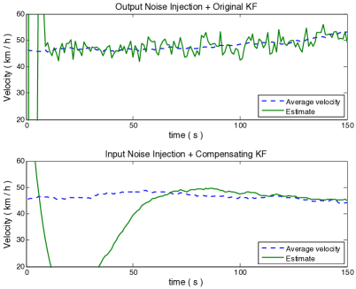
Figure 3: Two differentially private average velocity estimates, with $n=200$ users. The Kalman filters are initialized with the same incorrect initial mean velocity, in order to evaluate their convergence time.

VI Conclusion

We have discussed mechanisms for preserving the differential privacy of individual users transmitting measurements of their state trajectories to a trusted central server releasing sanitized filtered outputs based on these measurements. Decentralized versions of these mechanisms can in fact be implemented in the absence of trusted server by means of cryptographic techniques [17]. Further research on privacy issues associated with emerging large-scale information processing and control systems is critical to encourage their development. Moreover, obtaining a better understanding of the design trade-offs between privacy or security and performance in these systems raises interesting system theoretic questions.

References

- [1] G. W. Hart, “Nonintrusive appliance load monitoring,” Proceedings of the IEEE, vol. 80, no. 12, pp. 1870–1891, December 1992.
- [2] B. Hoh, T. Iwuchukwu, Q. Jacobson, M. Gruteser, A. Bayen, J.-C. Herrera, R. Herring, D. Work, M. Annavaram, and J. Ban, “Enhancing privacy and accuracy in probe vehicle based traffic monitoring via virtual trip lines,” IEEE Transactions on Mobile Computing, 2011.
- [3] J. A. Calandrino, A. Kilzer, A. Narayanan, E. W. Felten, and V. Shmatikov, ““you might also like”: Privacy risks of collaborative filtering,” in IEEE Symposium on Security and Privacy, 2001.
- [4] J. Le Ny and G. J. Pappas, “Differentially private filtering,” in Conference on Decision and Control, 2012, submitted.
- [5] C. Dwork, F. McSherry, K. Nissim, and A. Smith, “Calibrating noise to sensitivity in private data analysis,” in Proceedings of the Third Theory of Cryptography Conference, 2006, pp. 265–284.
- [6] S. P. Kasiviswanathan and A. Smith. (2008, March) A note on differential privacy: Defining resistance to arbitrary side information. [Online]. Available: http://arxiv.org/abs/0803.3946
- [7] D. Varodayan and A. Khisti, “Smart meter privacy using a rechargeable battery: minimizing the rate of information leakage,” in Proceedings of the IEEE International Conference on Acoustics, Speech, and Signal Processing, Prag, Czech Republic, 2011.
- [8] L. Sankar, S. R. Rajagopalan, and H. V. Poor, “A theory of privacy and utility in databases,” Princeton University, Tech. Rep., February 2011.
- [9] C. Dwork, “Differential privacy,” in Proceedings of the 33rd International Colloquium on Automata, Languages and Programming (ICALP), ser. Lecture Notes in Computer Science, vol. 4052. Springer-Verlag, 2006.
- [10] T. M. Cover and J. A. Thomas, Elements of Information Theory. New York, NY: John Wiley and Sons, 1991.
- [11] C. Dwork, K. Kenthapadi, F. McSherry, I. M. M. Naor, and Naor, “Our data, ourselves: Privacy via distributed noise generation,” Advances in Cryptology-EUROCRYPT 2006, pp. 486–503, 2006.
- [12] A. van der Schaft, L2-gain and passivity techniques in nonlinear control. Springer Verlag, 2000.
- [13] E. Shi, T.-H. H. Chan, E. Rieffel, R. Chow, and D. Song, “Privacy-preserving aggregation of time-series data,” in Proceedings of 18th Annual Network and Distributed System Security Symposium (NDSS 2011), February 2011.
- [14] B. D. O. Anderson and J. B. Moore, Optimal Filtering. Dover, 2005.
- [15] C. Scherer, P. Gahinet, and M. Chilali, “Multiobjective output-feedback control via LMI optimization,” IEEE Transactions on Automatic Control, vol. 42, no. 7, pp. 896–911, July 1997.
- [16] X. Sun, L. Munoz, and R. Horowitz, “Mixture Kalman filter based highway congestion mode and vehicle density estimator and its application,” in Proceedings of the American Control Conference, July 2004, pp. 2098–2103.
- [17] V. Rastogi and S. Nath, “Differentially private aggregation of distributed time-series with transformation and encryption,” in Proceedings of the ACM Conference on Management of Data (SIGMOD), Indianapolis, IN, June 2010.