Quick Hypervolume

Abstract

We present a new algorithm to calculate exact hypervolumes. Given a set of $d$-dimensional points, it computes the hypervolume of the dominated space. Determining this value is an important subroutine of Multiobjective Evolutionary Algorithms (MOEAs). We analyze the “Quick Hypervolume” (QHV) algorithm theoretically and experimentally. The theoretical results are a significant contribution to the current state of the art. Moreover the experimental performance is also very competitive, compared with existing exact hypervolume algorithms.

A full description of the algorithm is currently submitted to IEEE Transactions on Evolutionary Computation.

I Introduction

In this paper we focus on problems that optimize several objectives at the same time. Most of the times these objectives conflict with each other, meaning that maximizing one objective implies a loss of performance in another. An illustrative example of this problem is children’s Christmas gift lists. Children are usually not trying to maximize any particular objective, except possibly the number of gifts, and moreover are not mindful of the overall budget. Parents on the other hand are given the hard task of choosing which gift, or gifts, to buy. This is no trivial task, as the number of criteria/objectives involved is big. How much “fun” is the gift? In which case games are preferable to socks. Will it help in developing some talent? Where maybe books are preferable to games. Is it going to be useful? How long will it be in use? What is the cost per use? In which case, one might prefer socks. Of course children usually do not enjoy getting socks. Since the objectives are not measurable these problems are even harder than Multiobjective optimization problems.

As the number of objectives and of items under analysis increases, the complexity of the problem increases considerably. Namely the time the problem takes to be solved, due to the large number of possible choices. We seem to have intuitive knowledge of this complexity. From a psychological point of view this may have the negative impact of increasing anxiety [1]. Interestingly, as the amount of choice increases so do the artifacts people use for coping with complexity.

MOEAs [2] solve multiobjective optimization problems which occur in a wide range of problems, scheduling, economics, finance, automatic cell planning, traveling salesman, etc. Updated surveys on these algorithms are readily available [3, 4]. There is a class of MOEAs in which we are particularly interested because they use indicators to guide their decisions, namely they use the hypervolume [5, 6, 7, 8], or the generational distance.

We study the complexity of the algorithms that compute hypervolumes, specifically the space and time performance. We obtain the following results:

1. Section III describes a new, divide and conquer, algorithm for computing hypervolumes, QHV. The algorithm is fairly simple, although it requires some implementation details.

2. Section IV-A includes a theoretical analysis of QHV. Assuming the points are uniformly distributed on a hyper-sphere or hyper-plane, the analysis shows that QHV takes $O(dn^{1.1}\log^{d-2}n)$ time to solve an hypervolume problem, with $n$ points in $d$ dimensions. This bound holds for the average case, and with high probability. The power in $n$ converges to $1$, therefore it can also be bounded by $O(dn^{1.01}\log^{d-2}n)$ or less.

3. We study this performance experimentally. Our QHV prototype is extremely competitive against state of the art hypervolume algorithms, see Section IV-B.

Let us move on to the hypervolume problem.

II The Problem

Given a set of $d$-dimensional points we seek to compute the hypervolume of the dominated space. This section gives a precise description of the problem. Fig. 1 shows a set of points and the respective 2D hypervolume, commonly referred to as area.

Figure 1: The area of a set of 2D points.

The region of space under consideration is delimited by a rectangle with opposing vertexes $z$ and $o$, that are close to $0$ and $1$, respectively. We consider only rectangles that are parallel to the axis.

We say that point $p$ dominates point $a^{\prime}$ because $a^{\prime}$ is contained in the rectangle of vertexes $z$ and $p$. Notice that we cannot state that $d$ dominates $a^{\prime}$, since the rectangle with vertexes $z$ and $d$ does not contain $a^{\prime}$.

Given a set of points, in our example $\{a,a^{\prime},b,p,c,d\}$, we want to compute the dominated area, shown in gray in Fig. 1. In general we use hyperrectangles, instead of rectangles, to define dominance between points. The point $z$ is always a vertex of these hyper-rectangles. The opposing vertex is a point $p$, from the set. Therefore the problem is to compute the hypervolume occupied by the hyper-rectangles that use the points in the set, but without counting the dominated space twice, just like in the 2D example.

The coordinates can be any reals in $[0,1]$. Our algorithm uses a sub-routine to eliminate dominated points, so we do not insist on having a set of non-dominated points.

III Pivot Divide and Conquer

In this section we describe the QHV algorithm, by working our way from 2D to higher dimensions and gradually introduce the necessary concepts. Pivot divide and conquer is the technique used by QuickSort[9]. The process consists of the following three steps:

1. Select a “special” pivot point. This point is processed and excluded from the recursion.

2. Divide the space according to the pivot, more precisely classify points into the possible space regions.

3. Recursively solve each of the sub-problems in the “smaller” regions of space, and add up the hypervolumes.

III-A The 2D case

Fig. 2 shows an example of this process, in 2D. First we choose point $p$ to be the pivot. Second we divide the rectangle, of vertexes $z$ and $o$, according to $p$. Third we recursively compute the area of the points in quadrants $01$ and $10$.

Figure 2: Pivot Divide and Conquer for 2D points. The quadrants are labeled by binary numbers.

$\cdots$

IV Analysis

$\cdots$

IV-A Theoretical

$\cdots$

IV-A1 Average Case

There are certainly classes of problems that can not be modeled this way. Therefore we restrict our attention to hyper-planes and hyper-spheres with uniform point distribution, for which the model is appropriate.

Corollary 1

Consider a class of $d$-dimensional hypervolume problems of points uniformly distributed on a plane or on the surface of a hyper-sphere. For any positive number $\epsilon>0$, the optimistic QHV algorithm solves an $n$ point hypervolume problem, from this class, in $O(dn^{1+\epsilon}\log^{d-2}n)$ expected time.

$\cdots$

Corollary 2

Consider a class of $d$-dimensional hypervolume problems of points uniformly distributed on a plane or on the surface of a hyper-sphere. For any small positive number $\epsilon$, such that $0<\epsilon<1$, the optimistic QHV algorithm solves an $n$ point hypervolume problem, from this class, in $O(dn^{1+\epsilon}\log^{d-2}n)$ time, with at least $1-1/n$ probability. Formally:

$$Pr\left(T(n)<n^{1+\epsilon}\times O(d\log^{d-2}n)\right)\geq 1-\frac{1}{n}$$

where $T(n)$ is the time and $c$ a constant.

$\cdots$

IV-B Testing

We now present experimental results for estimating the overlap power and compare our QHV prototype with state of the art alternatives.

IV-B1 Experimental Setting

Let us now focus on the system time and space performance of the algorithm. In particular we will show how the techniques proposed in the previous section affect performance. Our implementation of the QHV algorithm is available at http://kdbio.inesc-id.pt/~lsr/QHV/

All results where obtained on a quad-core processor at 3.20GHz, with 256KB of L1 cache, 1MB of L2 cache, 8MB of L3 cache, and 8GB of main memory. The prototypes were compiled with gcc 4.7.1. For QHV we used -msse2 flag to support SSE2 and passed the cache line size into the code -DCLS=$$(getconf LEVEL1_DCACHE_LINESIZE), this was used to align memory to cache lines. The dimension was also determined at compile time, so there is a different binary for each dimension, this allows for better loop unrolling. Each one of the other prototypes contains a sophisticated makefile that produces optimized binaries, it automatically selects the best flags for a given platform. We used the optimized binaries produced by those makefiles, for our platform. Besides the proper flags we included -s -static -m32 -O9 -march=core2.

In the experimental evaluation we used the benchmarks available at http://www.wfg.csse.uwa.edu.au/hypervolume/, by While et al. [17]. In particular, we rely on the second benchmark with dimensions ranging from 3 to 13, with spherical, random, discontinuous and degenerate front datasets. Each dataset contains from 10 to 1000 points, depending on the number of dimensions. We performed 10 runs per dataset, each one with 20 fronts. The spherical points of the WFG dataset are not uniformly randomly chosen on a hyper-sphere’s surface with $d$ dimensions. To illustrate dimensions dependency, Fig. 3 shows a matrix of plots, each plot shows the points, plotted in 2D, by choosing two coordinates and discarding the rest.

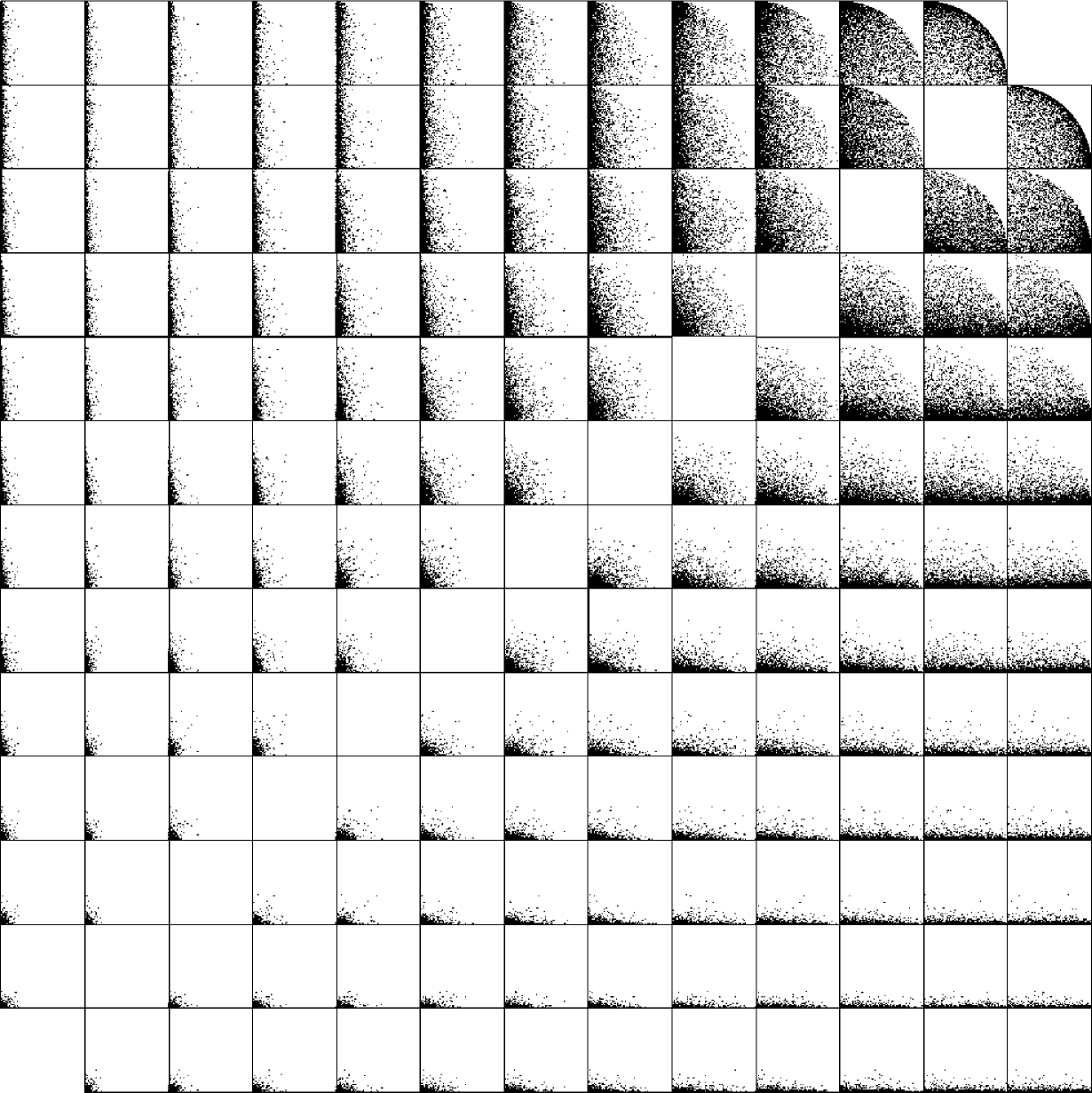
Figure 3: A matrix of plots for the 13D spherical points of the WFG dataset. The file contained around 300 points, a similar distribution can be observed in the remaining files of the dataset.

We also generated our own datasets, in such a way that the points where chosen uniformly at random on the hyper-sphere’s surface. More precisely we generated a random point in $[0,1]^{d}$, using the drand48 function, from stdlib.h. These points are uniformly random on the given space, but not necessarily on a hyper-sphere surface. We projected the points into the surface, by calculating the distance to the origin and dividing every coordinate by this value. Thus obtaining points at distance $1$. The resulting points can be seen in Fig. 4.

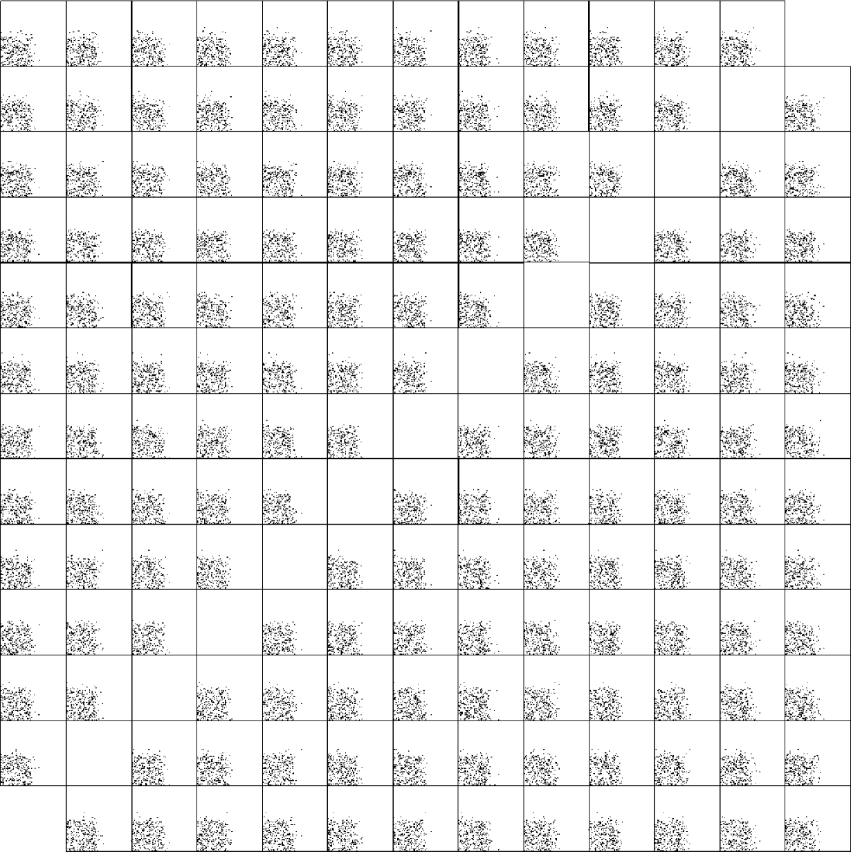
Figure 4: A matrix of plots for the 13D spherical points of our dataset. The file contained 300 points.

IV-B2 Experimental Performance

Figures 5–37 show the results concerning the running time of our QHV algorithm, the WFG algorithm [17], the FPRAS [35], with $\epsilon=0.01$, the HV algorithm, which is an improved version of FLP (http://iridia.ulb.ac.be/~manuel/hypervolume), and an optimized version for 4D, HV4D, provided by the authors [18]. We use logarithmic scales to cope with the gap in performance gap among different algorithms.

In comparing the performance of the different algorithms it is important to point out that the FPRAS returns an $\pm\epsilon$ approximation of the hypervolume, not an exact value. Moreover the approximation may miss this interval with 25% probability. This algorithm is extremely sensitive to $\epsilon$, changing it to $0.1$ yields a $100$ times speed-up, in practice. Therefore it is not meaningful to claim that the FPRAS is faster or slower in a given dataset, it depends on the precision that is required by the application. We choose a fixed reasonable $\epsilon$ to show how the performance evolves. The real hypervolume decreases exponentially with $d$, therefore the estimate should become inaccurate for higher dimensions. We inspected the resulting values and observed that estimates are actually reasonably accurate.

By far the worst performance of QHV occurs in the degenerated dataset. This is not an abnormal behavior of QHV. Instead the remaining algorithms behave much better than usual, for that kind of data set. Like QHV the FPRAS algorithm also maintains a consistent performance. Notice that for 10D the WFG algorithm is around 1000 times faster for this dataset than it is for the spherical dataset. Clearly QHV and the FPRAS are ignoring some intrinsic property of the dataset.

We can observe that HV is the fastest algorithm in 3D, but the performance degrades quickly. We omitted HV for higher dimensions, because of this slowdown. In 3D QHV is the second best algorithm. In 4D the fastest algorithm is the HV4D. QHV still obtains competitive performance, usually better than HV for a large number of points, except on the degenerated dataset. For higher dimensions, QHV is the fastest algorithm and the performance becomes similar to WFG for very high dimensions, for example 13D, Fig. 11. This is partially a consequence of the non-uniform dependencies on the data set. To show this fact we run a 13D test on our dataset, Figures  to  16. The results still show a large gap between WFG and QHV, where QHV remains faster. In 13D we tested less points, because the algorithms became $100$ times slower.

Note that at 13D the FPRAS obtains much better performance than QHV and WFG, partially because we did not applied a correction to $\epsilon$. The estimates are in fact fairly accurate, although without a theoretical guarantee.

In Table I we show the memory peak requirements of the different algorithms. It can be observed that, up to 7 dimensions, QHV requires less space than HV and WFG. The memory requirements of QHV increase with $d$, because we need to store a counter for each hyperoctant. As we mentioned in Section IV, this cost can be avoided by using a hash, which would also have an impact on the time performance. To avoid this effect we chose not to implement the hash. In fact the space requirements of these algorithms are modest, for example WFG loads all the point sets in a test into memory, to minimize this effect we reduced the tests so that they contain only one set of points. Although the memory peak increases for QHV the same happens to WFG, in 13 dimensions QHV also requires less space than WFG.

Heap Peaks in KB
	3D	4D	5D	6D	7D	10D	13D
QHV	28.7	37.0	66.3	129.3	242.3	795.1	311.8
WFG	125.1	195.4	273.6	359.6	453.3	781.5	1180.0
FPRAS	51.7	59.5	67.3	75.2	83.0	107.0	131.1
HV	168.2	199.5	230.8	262.1
HV4D		121.2
Stack Peaks in KB
QHV	2.4	2.4	4.8	4.9	7.1	12.4	16.3
WFG	9.5	9.5	9.5	9.5	9.5	9.5	9.5
FPRAS	1.4	1.4	1.4	1.4	1.4	1.4	1.4
HV	9.8	9.8	9.8	9.8
HV4D		9.6

TABLE I: Memory peaks of different algorithms on spherical fronts with 1000 points.

V Conclusions and Further Work

In this paper we proposed a new algorithm for computing hypervolumes, QHV. We focused on performance, time and space complexity. The QHV algorithm uses a divide and conquer strategy, which is different from the usual line sweep approach. The resulting algorithm is fairly simple and efficient. We analyzed QHV theoretically and experimentally.

V-A Conclusions

We expect the QHV algorithm to have a significant impact in the future development of MOEAs, in that it makes comparing more objectives feasible.

QHV is still devoid of extra features. Designing a version of QHV that can compute exclusive hypervolumes is an important unattended task. Other closely related problems may also benefit from the pivot divide and conquer strategy of QHV, namely computing empirical attainment functions [38].

Luís M. S. Russo received the Ph.D. degree from Instituto Superior Técnico, Lisbon, Portugal, in 2007. He is currently an Assistant Professor with Instituto Superior Técnico. His current research interests include algorithms and data structures for string processing and optimization.

Alexandre P. Francisco has a Ph.D. degree in Computer Science and Engineering and he is currently an Assistant Professor at the CSE Dept, IST, Tech Univ of Lisbon. His current research interests include the design and analysis of data structures and algorithms, with applications on network mining and large data processing.

Figure 5: 3D spherical fronts.

Figure 6: 4D spherical fronts.

Figure 7: 5D spherical fronts.

Figure 8: 6D spherical fronts.

Figure 9: 7D spherical fronts.

Figure 10: 10D spherical fronts.

Figure 11: 13D spherical fronts.

Figure 12: 3D spherical fronts, from our dataset.

Figure 13: 4D spherical fronts, from our dataset.

Figure 14: 5D spherical fronts, from our dataset.

Figure 15: 7D spherical fronts, from our dataset.

Figure 16: 13D spherical fronts, from our dataset.

Figure 17: 3D degenerated fronts.

Figure 18: 4D degenerated fronts.

Figure 19: 5D degenerated fronts.

Figure 20: 6D degenerated fronts.

Figure 21: 7D degenerated fronts.

Figure 22: 10D degenerated fronts.

Figure 23: 13D degenerated fronts.

Figure 24: 3D random fronts.

Figure 25: 4D random fronts.

Figure 26: 5D random fronts.

Figure 27: 6D random fronts.

Figure 28: 7D random fronts.

Figure 29: 10D random fronts.

Figure 30: 13D random fronts.

Figure 31: 3D discontinuous fronts.

Figure 32: 4D discontinuous fronts.

Figure 33: 5D discontinuous fronts.

Figure 34: 6D discontinuous fronts.

Figure 35: 7D discontinuous fronts.

Figure 36: 10D discontinuous fronts.

Figure 37: 13D discontinuous fronts.

References

- [1] B. Schwartz, The paradox of choice: why more is less, ser. P. S. Series. HarperCollins, 2005.
- [2] K. Deb, Multi-Objective Optimization Using Evolutionary Algorithms, ser. Wiley-Interscience series in systems and optimization. John Wiley & Sons, 2009.
- [3] A. Zhou, B. Qu, H. Li, S. Zhao, P. Suganthan, and Q. Zhang, “Multiobjective evolutionary algorithms: A survey of the state-of-the-art,” Swarm and Evolutionary Computation, 2011.
- [4] C. Goh, Y. Ong, and K. Tan, Multi-Objective Memetic Algorithms. Springer Verlag, 2009, vol. 171.
- [5] L. W. S. Huband, P. Hingston and L. Barone, “An evolution strategy with probabilistic mutation for multi-objective optimization,” in IEEE Congress on Evolutionary Computation, 2003, pp. 2284–2291.
- [6] D. C. J. Knowles and M. Fleischer, “Bounded archiving using the lebesgue measure,” in IEEE Congress on Evolutionary Computation, 2003, pp. 2490–2497.
- [7] N. B. M. Emmerich and B. Noujoks, “An emo algorithm using the hypervolume measure as selection criterion,” in Evolutionary Multi-Objective Optimization, 2005, pp. 62–76.
- [8] E. Zitzler and S. Künzli, “Indicator-based selection in multiobjective search,” in Parallel Problem Solving from Nature VIII, vol. 3242, 2004, pp. 832–842.
- [9] C. A. R. Hoare, “Algorithm 64: Quicksort,” Commun. ACM, vol. 4, pp. 321–, July 1961.
- [10] P. Briggs and L. Torczon, “An efficient representation for sparse sets,” ACM Letters on Programming Languages and Systems, vol. 2, pp. 59–69, 1993.
- [11] J. Bentley, Programming pearls. Addison-Wesley Professional, 2000.
- [12] A. Aho and J. Hopcroft, Design & Analysis of Computer Algorithms. Pearson Education India, 1974.
- [13] L. While, P. Hingston, L. Barone, and S. Huband, “A faster algorithm for calculating hypervolume,” Evolutionary Computation, IEEE Transactions on, vol. 10, no. 1, pp. 29 – 38, feb. 2006.
- [14] M. Mitzenmacher and E. Upfal, Probability and computing - randomized algorithms and probabilistic analysis. Cambridge University Press, 2005.
- [15] N. Beume and G. Rudolph, “S-metric calculation by considering dominated hypervolume as klee’s measure problem,” Evolutionary Computation, vol. 17, no. 4, pp. 477–492, 2009.
- [16] H. Yildiz and S. Suri, “On klee’s measure problem for grounded boxes,” in Proceedings of the 2012 symposuim on Computational Geometry, ser. SoCG ’12. New York, NY, USA: ACM, 2012, pp. 111–120.
- [17] L. B. L. While and L. Barone, “A fast way of calculating exact hypervolumes,” IEEE Transactions on Evolutionary Computation, no. 1, p. 99, 2011.
- [18] A. P. Guerreiro, C. M. Fonseca, and M. T. M. Emmerich, “A fast dimension-sweep algorithm for the hypervolume indicator in four dimensions,” in Proceedings of the 24th Canadian Conference on Computational Geometry, CCCG 2012, Charlottetown, Prince Edward Island, Canada, August 8-10, 2012, 2012, pp. 77–82.
- [19] J. Bader and E. Zitzler, “Hype: An algorithm for fast hypervolume-based many-objective optimization,” Evolutionary Computation, vol. 19, no. 1, pp. 45–76, 2011.
- [20] J. Wu and S. Azarm, “Metrics for quality assessment of a multiobjective design optimization solution set.” Journal of Mechanical Design(Transactions of the ASME), vol. 123, no. 1, pp. 18–25, 2001.
- [21] J. L. Bentley, “Multidimensional divide-and-conquer,” Commun. ACM, vol. 23, pp. 214–229, April 1980.
- [22] M. Fleischer, “The measure of pareto optima. applications to multi-objective metaheuristics,” in Evolutionary Multi-Criterion Optimization. Second International Conference, EMO 2003. Springer, 2003, pp. 519–533.
- [23] C. Fonseca, L. Paquete, and M. Lopez-Ibanez, “An optimal algorithm for a special case of Klee’s measure problem in three dimensions,” Centre for Intelligent Systems, University of Algarve, Faro, Potugal, Tech. Rep. CSI-RT-I-01/2006, 2006.
- [24] C. Fonseca, L. Paquete, and M. Lopez-Ibanez, “An improved dimension-sweep algorithm for the hypervolume indicator,” in Evolutionary Computation, 2006. CEC 2006. IEEE Congress on, july 2006, pp. 1157 – 1163.
- [25] L. While, L. Bradstreet, L. Barone, and P. Hingston, “Heuristics for optimizing the calculation of hypervolume for multi-objective optimization problems,” in Evolutionary Computation, 2005. The 2005 IEEE Congress on, vol. 3, sept. 2005, pp. 2225 – 2232 Vol. 3.
- [26] V. Klee, “Can the measure of be computed in less than steps?” The American Mathematical Monthly, vol. 84, no. 4, pp. 284–285, April 1977.
- [27] J. L. Bentley, “Algorithms for klee’s rectangle problems,” 1977, carnegie Mellon Univ., Comput. Sci. Dept.
- [28] M. Overmars and C.-K. Yap, “New upper bounds in klee’s measure problem,” in Foundations of Computer Science, 1988., 29th Annual Symposium on, oct 1988, pp. 550 –556.
- [29] N. Beume, “Hypervolumen-basierte selektion in einem evolutionären algorithmus zur mehrzieloptimierung,” 2006.
- [30] L. Bradstreet, L. While, and L. Barone, “A fast many-objective hypervolume algorithm using iterated incremental calculations,” in Evolutionary Computation (CEC), 2010 IEEE Congress on, july 2010, pp. 1 –8.
- [31] N. Beume, C. Fonseca, M. López-Ibáñez, L. Paquete, and J. Vahrenhold, “On the complexity of computing the hypervolume indicator,” Evolutionary Computation, IEEE Transactions on, vol. 13, no. 5, pp. 1075–1082, 2009.
- [32] L. Bradstreet, L. While, and L. Barone, “A fast incremental hypervolume algorithm,” Evolutionary Computation, IEEE Transactions on, vol. 12, no. 6, pp. 714–723, 2008.
- [33] Q. Yang and S. Ding, “Novel algorithm to calculate hypervolume indicator of pareto approximation set,” in Advanced Intelligent Computing Theories and Applications, ser. Communications in Computer and Information Science, 2007, vol. 2, pp. 235–244.
- [34] A. Guerreiro, “Efficient algorithms for the assessment of stochastic multiobjective optimizers,” Ph.D. dissertation, Master’s thesis, IST, Technical University of Lisbon, Portugal, 2011.
- [35] K. Bringmann and T. Friedrich, “Approximating the volume of unions and intersections of high-dimensional geometric objects,” Computational Geometry, vol. 43, no. 6, pp. 601–610, 2010.
- [36] K. Bringmann and T. Friedrich, “An efficient algorithm for computing hypervolume contributions,” Evolutionary Computation, vol. 18, no. 3, pp. 383–402, 2010.
- [37] K. Bringmann and T. Friedrich, “Approximating the least hypervolume contributor: NP-hard in general, but fast in practice,” in EMO, ser. Lecture Notes in Computer Science, M. Ehrgott, C. M. Fonseca, X. Gandibleux, J.-K. Hao, and M. Sevaux, Eds., vol. 5467. Springer, 2009, pp. 6–20.
- [38] V. Grunert da Fonseca, C. Fonseca, and A. Hall, “Inferential performance assessment of stochastic optimisers and the attainment function,” in Evolutionary Multi-Criterion Optimization, ser. Lecture Notes in Computer Science. Springer Berlin / Heidelberg, 2001, vol. 1993, pp. 213–225.