Digital double barrier options: Several barrier periods and structure floors

Abstract.

We determine the price of digital double barrier options with an arbitrary number of barrier periods in the Black-Scholes model. This means that the barriers are active during some time intervals, but are switched off in between. As an application, we calculate the value of a structure floor for structured notes whose individual coupons are digital double barrier options. This value can also be approximated by the price of a corridor put.

1. Introduction

We consider digital double barrier options with an arbitrary number of barrier periods. This means that the holder receives the payoff only if the underlying stays between the two barriers in certain specified time intervals. While such contracts might make sense by themselves (as a weather or energy derivative with seasonal barriers, say), our motivation is to use them for the pricing of certain structured notes with several coupons. Such trades often feature an aggregate floor at the final coupon date, which increases the total payoff to a guaranteed amount if the sum of the coupons is less than this amount. Pricing this terminal premium requires the law of the sum of the coupons, which can be recovered from its moments. If the individual coupons of the note are digital barrier options, then these moments can be computed from the prices of options of the kind described above, where the sets of barrier periods are subsets of the coupon periods of the note.

Recall that Monte Carlo pricing of barrier contracts is tricky, because the discretization produces a downward bias for the barrier hitting probability. For single barrier options, this difficulty can be overcome using the explicit law of the maximum of the Brownian bridge [1, 3]. For double barrier options, the exit probability of the Brownian bridge is not known; see Baldi et al. [2] for an approximate approach using sample path large deviations. These numerical challenges led us to investigate exact valuation formulas.

The paper is structured as follows. In Section 2 we define the payoffs we are interested in and price them for a single barrier period. Section 3 extends the result to arbitrarily many periods of active barriers. Our main application, namely the pricing of structure floors, is presented in Section 4. Since our exact pricing formula is fairly involved, we consider an asymptotic approximation for a large number of periods in Section 5.

2. Preliminaries and pricing for one period

We assume that the underlying $(S_{t})_{t\geq 0}$ has the risk-neutral dynamics

$$dS_{t}/S_{t}=rdt+\sigma dW_{t}$$

with constant interest rate $r>0$, volatility $\sigma>0$ and a standard Brownian motion $W$. Consider a digital barrier option with two barriers $B_{\mathrm{low}}$ and $B_{\mathrm{up}}$ that are activated at time $T_{0}>0$ and stay active for a time period of length $P>0$. At maturity $T_{0}+P$, the payoff is one unit of currency if the underlying has stayed between the two barriers:

(1) $$C_{1}:=\mathbf{1}_{\{B_{\mathrm{low}}<S_{t}<B_{\mathrm{up}},\ t\in[T_{0},T_{0}+P]\}}.$$

Let us denote the price of this “one-period double barrier digital” by

(2) $$BD(S_{t},t;\{T_{0}\},P,B_{\mathrm{low}},B_{\mathrm{up}},r):=e^{-r(T_{0}+P)}\mathbf{E}[C_{1}],$$

where $\mathbf{E}$ is the expectation w.r.t. the pricing measure $\mathbf{P}$. In the terminology of Hui [7], this is a rear-end barrier option, because the two barriers are alive only towards the end of the contract, namely between $T_{0}$ and maturity $T_{0}+P$. Hui [7] has determined the price for a barrier call of this kind. The digital case is a simple modification, but we go through it to prepare the calculation of the price for several barrier periods (see Section 3). The value function

$$f(S,t):=BD(S,t;\{T_{0}\},P,B_{\mathrm{low}},B_{\mathrm{up}},r)$$

satisfies the Black-Scholes PDE

$$\frac{\partial f}{\partial t}+\frac{1}{2}\sigma^{2}S^{2}\frac{\partial^{2}f}{\partial S^{2}}+rS\frac{\partial f}{\partial S}-rf=0$$

with the terminal condition $f(S,T_{0}+P)=1$, for $S\in(B_{\mathrm{low}},B_{\mathrm{up}})$, and the boundary conditions $f(B_{\mathrm{low}},t)=f(B_{\mathrm{up}},t)=0$ for $t\in[T_{0},T_{0}+P]$. We use the standard transformation $f(S,t)=e^{\alpha x+\beta\tau}U(x,\tau)$, where

(3) $$x :=\log(S/B_{\mathrm{low}}),\qquad\tau:=\tfrac{1}{2}\sigma^{2}(T_{0}+P-t),$$

$$\alpha :=-\frac{1}{2}\left(\frac{2}{\sigma^{2}}r-1\right),\qquad\beta:=-\frac{2r}{\sigma^{2}}-\alpha^{2},$$

to transform the Black-Scholes PDE into the heat equation

(4) $$\frac{\partial^{2}U}{\partial{x}^{2}}=\frac{\partial U}{\partial\tau}.$$

The time points $(0,T_{0},T_{0}+P)$ are thus converted to $(\tfrac{1}{2}\sigma^{2}(T_{0}+P),p,0)$, where $p:=\tfrac{1}{2}\sigma^{2}P$ is the barrier period length in the new time scale. The boundary conditions in the new coordinates are

(5) $$U(0,\tau)=U(L,\tau)=0,\qquad\tau\in[0,p],$$

where $L:=\log(B_{\mathrm{up}}/B_{\mathrm{low}})$. The terminal condition translates to the initial condition

(6) $$U(x,0)=e^{-\alpha x},\qquad x\in(0,L).$$

Proposition 1.

For $0<t<T_{0}$, the price of a barrier digital with barrier period $[T_{0},T_{0}+P]$ and payoff $C_{1}$ at $T_{0}+P$ (see (1)) is

(7) $$BD(S,t;\{T_{0}\},P,B_{\mathrm{low}},B_{\mathrm{up}},r)=\sqrt{2\pi}\left(\frac{S}{B_{\mathrm{low}}}\right)^{\alpha}\sum_{k=1}^{\infty}k\frac{1-(-1)^{k}e^{-\alpha L}}{\alpha^{2}L^{2}+k^{2}\pi^{2}}e^{-(\frac{k\pi}{L})^{2}p+\beta\tau}\\ \cdot\int_{-\frac{x}{\sqrt{2(\tau-p)}}}^{\frac{L-x}{\sqrt{2(\tau-p)}}}\sin\left(\frac{k\pi}{L}(x+y\sqrt{2(\tau-p)})\right)e^{-y^{2}/2}dy.$$

Proof.

We have to solve the problem (4)–(6). First consider the rectangle $(0,L)\times(0,p)$. There the solution can be found by separation of variables [5, Section 4.1]:

(8) $$U(x,\tau)=\sum_{k=1}^{\infty}b_{k}\sin\left(\frac{k\pi}{L}x\right)e^{-(\frac{k\pi}{L})^{2}\tau},\qquad(x,\tau)\in(0,L)\times(0,p),$$

where

$$b_{k}:=\frac{2}{L}\int_{0}^{L}e^{-\alpha x_{1}}\sin\left(\frac{k\pi}{L}x_{1}\right)dx_{1}=2k\pi\frac{1-(-1)^{k}e^{-\alpha L}}{\alpha^{2}L^{2}+k^{2}\pi^{2}}$$

are the Fourier coefficients of the boundary function $U(x,0)=e^{-\alpha x}$. At $\tau=p$, the solution is given by (8) for $0<x<L$ and vanishes otherwise. Inserting $\tau=p$ into (8) yields

(9) $$U(x,p)=\begin{cases}\sum_{k=1}^{\infty}2k\pi\frac{1-(-1)^{k}e^{-\alpha L}}{\alpha^{2}L^{2}+k^{2}\pi^{2}}\sin(\frac{k\pi}{L}x)e^{-(\frac{k\pi}{L})^{2}p},&0<x<L\\ 0,&x\leq 0\ \text{or}\ x\geq L.\end{cases}$$

Now we solve for $U$ in the region $\mathbb{R}\times(p,\tfrac{1}{2}\sigma^{2}(T_{0}+P))$. There are no boundary conditions here, since the barriers are not active in the interval $(0,T_{0})$ (in the original time scale). The solution is found by convolving the initial condition (9) with the heat kernel [5, 2.3.1.b]:

$$U(x,\tau) =\frac{1}{\sqrt{2\pi}}\int_{-\infty}^{\infty}U(x+y\sqrt{2(\tau-p)},p)e^{-y^{2}/2}dy$$

(10) $$=\frac{1}{\sqrt{2\pi}}\int_{-\frac{x}{\sqrt{2(\tau-p)}}}^{\frac{L-x}{\sqrt{2(\tau-p)}}}U(x+y\sqrt{2(\tau-p)},p)e^{-y^{2}/2}dy.$$

Inserting (9) and rearranging yields (7). ∎

3. Double barrier digitals with arbitrarily many periods

For $n$ tenor dates

$$0<T_{0}<\dots<T_{n-1}$$

and a fixed period length $P>0$, we consider a contract that pays one unit of currency at time $T_{n-1}+P$, if the underlying has remained between the two barriers $B_{\mathrm{low}}$ and $B_{\mathrm{up}}$ during each of the time intervals $[T_{i},T_{i}+P]$, $i=0,\dots,n-1$. By the risk-neutral pricing formula, the price of this “multi-period double barrier digital” is given by

(11) $$BD(S_{t},t;\{T_{0},\dots,T_{n-1}\},P,B_{\mathrm{low}},B_{\mathrm{up}},r):=e^{-r(T_{n-1}+P)}\mathbf{E}\left[\prod_{i=1}^{n}C_{i}\right],$$

where

$$C_{i}:=\mathbf{1}_{\{B_{\mathrm{low}}<S_{t}<B_{\mathrm{up}},\ t\in[T_{i-1},T_{i-1}+P]\}}.$$

To calculate the price, we use the coordinate change (3) again. The $n$ barrier periods $[T_{i},T_{i}+P]$ are mapped to $[\tau_{i},\tau_{i}+p]$, where

$$\tau_{i}:=\tfrac{1}{2}\sigma^{2}(T_{n-1}-T_{i-1}),\qquad i=n,\dots,1,$$

are the images of the barrier period endpoints under the coordinate change (see Figure 1).

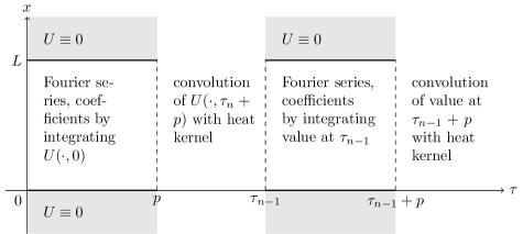
Figure 1. Solving the boundary value problem for an arbitrary number of barrier periods.

Define the following auxiliary functions:

$$h_{j}(k_{1},\dots,k_{j+1};x_{1},\dots,x_{j+1};y_{1},\dots,y_{j+1};x,\tau)\\ :=\tfrac{1}{\sqrt{2\pi}}e^{-y_{j+1}^{2}/2}\ \mathbf{1}_{\left[-\tfrac{x}{\sqrt{2(\tau-(\tau_{n-j}+p))}},\tfrac{L-x}{\sqrt{2(\tau-(\tau_{n-j}+p))}}\right]}(y_{j+1})\\ \cdot g_{j}(k_{1},\dots,k_{j+1};x_{1},\dots,x_{j+1};y_{1},\dots,y_{j};x+y_{j+1}\sqrt{2(\tau-(\tau_{n-j}+p))},\tau_{n-j}+p)$$

and

$$g_{j}(k_{1},\dots,k_{j+1};x_{1},\dots,x_{j+1};y_{1},\dots,y_{j};x,\tau)\\ :=\tfrac{2}{L}\sin\tfrac{k_{j+1}\pi x_{j+1}}{L}\sin\tfrac{k_{j+1}\pi x}{L}e^{-(k_{j+1}\pi/L)^{2}(\tau-\tau_{n-j})}\\ \cdot h_{j-1}(k_{1},\dots,k_{j};x_{1},\dots,x_{j};y_{1},\dots,y_{j};x_{j+1},\tau_{n-j}),$$

with the recursion starting at

(12) $$g_{0}(k_{1};x_{1};;x,\tau):=\tfrac{2}{L}e^{-\alpha x_{1}}\sin\tfrac{k_{1}\pi x_{1}}{L}\sin\tfrac{k_{1}\pi x}{L}e^{-(k_{1}\pi/L)^{2}\tau}.$$

The following theorem contains our pricing formula. The first formula (13) is for time points inside a barrier period, whereas the second expression (14) holds for valuation times where the barriers are not active.

Theorem 2.

The value function (11) equals $e^{\alpha x+\beta\tau}U(x,\tau)$, where for $0\leq j<n$, $\tau_{n-j}\leq\tau\leq\tau_{n-j}+p$, $0<x<L$, we have

(13) $$U(x,\tau)=\underbrace{\int_{-\infty}^{\infty}\dots\int_{-\infty}^{\infty}}_{j}\underbrace{\int_{0}^{L}\dots\int_{0}^{L}}_{j+1}\sum_{k_{1}=0}^{\infty}\dots\sum_{k_{j+1}=0}^{\infty}\\ g_{j}(k_{1},\dots,k_{j+1};x_{1},\dots,x_{j+1};y_{1},\dots,y_{j};x,\tau)dx_{1}\dots dx_{j+1}dy_{1}\dots dy_{j},$$

whereas for $0\leq j<n$, $\tau_{n-j}+p<\tau<\tau_{n-(j+1)}$ (with $\tau_{0}:=\infty$), $x\in\mathbb{R}$, we have

(14) $$U(x,\tau)=\underbrace{\int_{-\infty}^{\infty}\dots\int_{-\infty}^{\infty}}_{j+1}\underbrace{\int_{0}^{L}\dots\int_{0}^{L}}_{j+1}\sum_{k_{1}=0}^{\infty}\dots\sum_{k_{j+1}=0}^{\infty}\\ h_{j}(k_{1},\dots,k_{j+1};x_{1},\dots,x_{j+1};y_{1},\dots,y_{j+1};x,\tau)dx_{1}\dots dx_{j+1}dy_{1}\dots dy_{j+1}.$$

Proof.

The idea is to iterate the argument of Proposition 1 (see Figure 1). We use separation of variables in the barrier periods, and convolution with the heat kernel for the periods in between. The required initial condition at the left boundary comes from the previous step of the iteration (for $j=0$ also from the payoff, of course).

For $j=0$, formula (13) is identical to (8). To show (14) for $j=0$, let $p<\tau<\tau_{n-1}$ (recall that $\tau_{n}=0$) and $x\in\mathbb{R}$, and use (10) and (8) to obtain

$$U(x,\tau) =\frac{1}{\sqrt{2\pi}}\int_{-\frac{x}{\sqrt{2(\tau-p)}}}^{\frac{L-x}{\sqrt{2(\tau-p)}}}U(x+y_{1}\sqrt{2(\tau-p)},p)e^{-y_{1}^{2}/2}dy_{1}$$

$$=\frac{1}{\sqrt{2\pi}}\int_{-\infty}^{\infty}\mathbf{1}_{\left[-\tfrac{x}{\sqrt{2(\tau-p)}},\tfrac{L-x}{\sqrt{2(\tau-p)}}\right]}(y_{1})$$

$$\qquad\qquad\int_{0}^{L}\sum_{k_{1}=0}^{\infty}g_{0}(k_{1};x_{1};;x+y_{1}\sqrt{2(\tau-p)},p)e^{-y_{1}^{2}/2}dx_{1}dy_{1}$$

$$=\int_{-\infty}^{\infty}\int_{0}^{L}\sum_{k_{1}=0}^{\infty}h_{0}(k_{1};x_{1};y_{1};x,\tau)dx_{1}dy_{1}.$$

This is (14) for $j=0$.

Next consider a rectangle

(15) $$(\tau,x)\in(\tau_{n-j},\tau_{n-j}+p)\times(0,L),\qquad 1\leq j<n.$$

At the left boundary, the solution is $x_{j+1}\mapsto U(x_{j+1},\tau_{n-j})$. By the induction hypothesis, it equals (14) with $j$ replaced by $j-1$:

(16) $$U(x_{j+1},\tau_{n-j})=\underbrace{\int_{-\infty}^{\infty}\dots\int_{-\infty}^{\infty}}_{j}\underbrace{\int_{0}^{L}\dots\int_{0}^{L}}_{j}\sum_{k_{1}=0}^{\infty}\dots\sum_{k_{j}=0}^{\infty}\\ h_{j-1}(k_{1},\dots,k_{j};x_{1},\dots,x_{j};y_{1},\dots,y_{j};x_{j+1},\tau_{n-j})dx_{1}\dots dx_{j}dy_{1}\dots dy_{j}.$$

The solution in the rectangle (15) is thus obtained by separation of variables as

(17) $$U(x,\tau)=\sum_{k_{j+1}=0}^{\infty}b_{k_{j+1}}\sin\left(\frac{k_{j+1}\pi}{L}x\right)e^{-(\frac{k_{j+1}\pi}{L})^{2}(\tau-\tau_{n-j})},$$

where

(18) $$b_{k_{j+1}}:=\frac{2}{L}\int_{0}^{L}U(x_{j+1},\tau_{n-j})\sin\left(\frac{k_{j+1}\pi}{L}x_{j+1}\right)dx_{j+1}$$

denote now the Fourier coefficients of $x_{j+1}\mapsto U(x_{j+1},\tau_{n-j})$. Inserting (16) into (18) and then (18) into (17) yields (13), by the definition of $g_{j}$.

Finally, consider a strip

(19) $$(\tau,x)\in(\tau_{n-j}+p,\tau_{n-(j+1)})\times\mathbb{R},\qquad 1\leq j<n.$$

At the left boundary, we use (13) as induction hypothesis. The solution thus vanishes for $x\notin(0,L)$, and for $\tau=\tau_{n-j}+p$ and $x\in(0,L)$ it is

(20) $$U(x,\tau_{n-j}+p)=\underbrace{\int_{-\infty}^{\infty}\dots\int_{-\infty}^{\infty}}_{j}\underbrace{\int_{0}^{L}\dots\int_{0}^{L}}_{j+1}\sum_{k_{1}=0}^{\infty}\dots\sum_{k_{j+1}=0}^{\infty}\\ g_{j}(k_{1},\dots,k_{j+1};x_{1},\dots,x_{j+1};y_{1},\dots,y_{j};x,\tau_{n-j}+p)dx_{1}\dots dx_{j+1}dy_{1}\dots dy_{j}.$$

As above, the solution in the strip (19) is found by convolution with the heat kernel:

$$U(x,\tau)=\frac{1}{\sqrt{2\pi}}\int_{-\infty}^{\infty}\mathbf{1}_{\left[-\tfrac{x}{\sqrt{2(\tau-(\tau_{n-j}-p))}},\tfrac{L-x}{\sqrt{2(\tau-(\tau_{n-j}-p))}}\right]}(y_{j+1})\\ \qquad U(x+y_{j+1}\sqrt{2(\tau-(\tau_{n-j}-p))},\tau_{n-j}-p)e^{-y_{j+1}^{2}/2}dy_{j+1}.$$

Now insert (20), with $x$ replaced by $x+y_{j+1}\sqrt{2(\tau-(\tau_{n-j}+p))}$, and use the definition of $h_{j}$ to conclude (14). ∎

Note that Proposition 1 corresponds to (14) for $j=0$. As seen there, the integral $\int_{0}^{L}dx_{1}$ can be done in closed form. We have not included this evaluation in Theorem 2 to increase its readability.

If a different option (a call, say) with the same barrier conditions is to be priced instead of a digital payoff, the quantity $e^{-\alpha x_{1}}$ in (12) should be replaced by the appropriate payoff $U(x_{1},0)$.

4. Structure floors

In this section we assume that our tenor structure satisfies $T_{i-1}+P=T_{i}$ for $1\leq i<n$, and define $T_{n}:=T_{n-1}+P$. We consider a structured note with $n$ coupons, where the $i$-th coupon consists of a payment of

(21) $$C_{i}=\mathbf{1}_{\{B_{\mathrm{low}}<S_{t}<B_{\mathrm{up}},\ t\in[T_{i-1},T_{i}]\}},\qquad 1\leq i\leq n,$$

at time $T_{i}$. These coupons can be priced by Proposition 1 (replace $T_{0}$ by $T_{i-1}$). In addition, the holder receives the terminal premium

(22) $$\left(F-\sum_{i=1}^{n}C_{i}\right)^{+}$$

at $T_{n}$, where $F>0$. This means that the aggregate payoff $A:=\sum_{i=1}^{n}C_{i}$ of the note is floored at $F$, which is a popular feature of structured notes. While the individual coupons are straightforward to valuate, it is less obvious how to get a handle on the law of $A$. We now show that this law is linked to barrier options with several barrier periods. Indeed, the following result is based on the fact that the moments

(23) $$\mathbf{E}[A^{\nu}]=\sum_{i=0}^{n}i^{\nu}\mathbf{P}[A=i],\qquad 1\leq\nu<n,$$

of $A$ are linear combinations of multi-period double barrier option prices, with coefficients

(24) $$c(\nu,J):=\sum_{\begin{subarray}{c}0\leq i_{1},\dots,i_{n}\leq\nu\\ \mathrm{supp}(\mathbf{i})=J\end{subarray}}\binom{\nu}{i_{1},\dots,i_{n}},\qquad J\subseteq\{1,\dots,n\}.$$

(The notation $\mathrm{supp}(\mathbf{i})=J$ means that $J$ is the set of indices such that the corresponding components of the vector $\mathbf{i}=(i_{1},\dots,i_{n})$ are non-zero.)

Theorem 3.

The price of the structure floor (22) at time $t<T_{0}$ can be expressed as

(25) $$e^{-r(T_{n}-t)}\mathbf{E}[(F-A)^{+}]=e^{-r(T_{n}-t)}\sum_{i=0}^{n\wedge\lfloor F\rfloor}(F-i)\mathbf{P}[A=i],$$

where

(26) $$\mathbf{P}[A=n]=BD(S_{t},t;\{T_{0}\},T_{n}-T_{0},B_{\mathrm{low}},B_{\mathrm{up}},0).$$

The other point masses $\mathbf{P}[A=i]$ in (25) can be recovered from the moments of $A$ by solving (23) (including $\nu=0$, of course). The moments in turn can be computed from barrier digital prices by ($1\leq\nu<n$)

(27) $$\mathbf{E}[A^{\nu}]=\sum_{J\subseteq\{1,\dots,n\}}c(\nu,J)\cdot BD(S_{t},t;\{T_{j}:j\in J\},P,B_{\mathrm{low}},B_{\mathrm{up}},0),$$

where the coefficients $c(\nu,J)$ are defined in (24).

Proof.

The expression (25) is clear. The event in (26) means that all of the $n$ coupons (21) are paid. By our assumption that $T_{i}=T_{i-1}+P$, its risk-neutral probability is the (undiscounted) price of a double barrier digital with one barrier period $[T_{0},T_{n}]$, which yields (26). To prove (27), we calculate

$$\mathbf{E}[A^{\nu}]=\mathbf{E}\left[\left(\sum_{i=1}^{n}C_{i}\right)^{\nu}\right] =\sum_{i_{1},\dots,i_{n}}\binom{\nu}{i_{1},\dots,i_{n}}\mathbf{E}[C_{1}^{i_{1}}\dots C_{n}^{i_{n}}]$$

$$=\sum_{i_{1},\dots,i_{n}}\binom{\nu}{i_{1},\dots,i_{n}}\mathbf{E}\bigg{[}\prod_{\begin{subarray}{c}j=1\\ i_{j}>0\end{subarray}}^{n}C_{j}\bigg{]}$$

$$=\sum_{J\subseteq\{1,\dots,n\}}\Bigg{(}\sum_{\begin{subarray}{c}i_{1},\dots,i_{n}\\ \mathrm{supp}(\mathbf{i})=J\end{subarray}}\binom{\nu}{i_{1},\dots,i_{n}}\Bigg{)}\mathbf{E}\Big{[}\prod_{j\in J}C_{j}\Big{]}.$$

Now observe that $\prod_{j\in J}C_{j}$ is the payoff of a double barrier digital with barrier periods $[T_{j},T_{j}+P]$ for $j\in J$. ∎

When calculating the value $BD$ in (27) for, say, $J=\{1,2,4,5,6\}$, the adjacent barrier periods should be concatenated: Do not compute the price for five barrier periods of length $P$, but rather for two periods with lengths $2P$ and $3P$. We did not include this obvious extension (barrier periods of variable length) in Theorem 2 in order not to complicate an already heavy notation.

5. Approximation by a corridor option

Theorems 2 and 3 express the price of the structure floor (22) by iterated sums and integrals. Due to the factors of order $e^{-k_{j}^{2}}$, the infinite series $\sum_{k_{j}}$ may be truncated after just a few terms. Still, numerical quadrature may be too involved for a large number of coupons, so we present an approximation. Let us fix a maturity $T=T_{n}$ and assume that the $n$ coupon periods

$$\mathcal{T}_{i}^{n}:=[\tfrac{i-1}{n}T,\tfrac{i}{n}T],\qquad 1\leq i\leq n,$$

have length $T/n$. For large $n$, the proportion of intervals during which the underlying stays inside the barrier interval

$$\mathcal{B}:=[B_{\mathrm{low}},B_{\mathrm{up}}]$$

is similar to the proportion of time that the underlying spends inside $\mathcal{B}$, i.e., the occupation time. This is made precise in the following result, which holds not only for the Black-Scholes model, but for virtually any continuous model. Note that the level sets of geometric Brownian motion have a.s. measure zero (cf. [8, Theorem 2.9.6]).

Theorem 4.

Let $(S_{t})_{t\geq 0}$ be a continuous stochastic process such that for each real $c$ the level set $\{t:S_{t}=c\}$ has a.s. Lebesgue measure zero. Then we have a.s.

$$\lim_{n\to\infty}\frac{1}{n}\sum_{i=1}^{n}\mathbf{1}_{\{S_{t}\in\mathcal{B}\ \forall t\in\mathcal{T}_{i}^{n}\}}=\int_{0}^{T}\mathbf{1}_{\mathcal{B}}(S_{t})dt.$$

Proof.

For $1\leq i\leq n$, define processes $(X_{ni}(t))_{0\leq t\leq T}$ by

$$X_{ni}(t):=\begin{cases}1&\text{if}\ t\in\mathcal{T}_{i}^{n}\ \text{and}\ S_{u}\in\mathcal{B}\ \forall u\in\mathcal{T}_{i}^{n}\\ 0&\text{otherwise}.\end{cases}$$

Put $X_{n}:=\sum_{i=1}^{n}X_{ni}$. We claim that, a.s., the function $X_{n}(\cdot)$ converges pointwise on the set $[0,T]\setminus\{t:S_{t}=B_{\mathrm{low}}\ \text{or}\ S_{t}=B_{\mathrm{up}}\}$, with limit $\mathbf{1}_{\mathcal{B}}(S_{\cdot})$. Indeed, if $t\in[0,T]$ is such that $S_{t}\notin\mathcal{B}$, then $X_{n}(t)=0$ for all $n$. If, on the other hand, $S_{t}\in\mathrm{int}(\mathcal{B})$, then $t$ has a neighborhood $V$ such that $S_{u}\in\mathcal{B}$ for all $u\in V,$ by continuity. Hence $X_{n}(t)=1$ for large $n$. Since we have pointwise convergence on a set of (a.s.) full measure, we can apply the dominated convergence theorem to conclude

$$\lim_{n\to\infty}\int_{0}^{T}X_{n}(t)dt=\int_{0}^{T}\mathbf{1}_{\mathcal{B}}(S_{t})dt,\qquad\text{a.s.}$$

But this is the desired result, since

$$\int_{0}^{T}X_{n}(t)dt =\sum_{i=1}^{n}\int_{0}^{T}X_{ni}(t)dt$$

$$=\sum_{i=1}^{n}\int_{\mathcal{T}_{i}^{n}}X_{ni}(t)dt$$

$$=\sum_{i=1}^{n}|\mathcal{T}_{i}^{n}|\ \mathbf{1}_{\{S_{t}\in\mathcal{B}\ \forall t\in\mathcal{T}_{i}^{n}\}}=\frac{1}{n}\sum_{i=1}^{n}\mathbf{1}_{\{S_{t}\in\mathcal{B}\ \forall t\in\mathcal{T}_{i}^{n}\}}.$$

∎

Theorem 4 suggests the approximation

(28) $$e^{-rT}\mathbf{E}(F-A)^{+}\approx ne^{-rT}\mathbf{E}\left(\frac{F}{n}-\int_{0}^{T}\mathbf{1}_{\mathcal{B}}(S_{t})dt\right)^{+}$$

for the price of the structure floor (22). It is obtained from replacing $F$ by $F/n$ in the relation

$$\mathbf{E}(nF-A)^{+}\sim n\mathbf{E}\left(F-\int_{0}^{T}\mathbf{1}_{\mathcal{B}}(S_{t})dt\right)^{+},$$

which follows from Theorem 4. On the right hand side of (28) we recognize the price of a put on the occupation time of $(S_{t})$, also called a corridor option. Fusai [6] studied such options in the Black-Scholes model. In particular, his Theorem 1 gives an expression for the characteristic function of $\int_{0}^{T}\mathbf{1}_{\mathcal{B}}(S_{t})dt$. Since the formula is rather involved, we do not reproduce it here. Section 4 of Fusai [6] explains how to compute the corridor option price from the characteristic function by numerical Laplace inversion.

This approximation holds for period lengths tending to zero. One could also let the number of coupons tend to infinity for a fixed period length $P$, so that maturity increases linearly with $n$. The dependence of the random variables $C_{i}$ and $C_{j}$ decreases for large $|i-j|$, and so we conjecture a central limit theorem, i.e., that

$$\frac{A-\mathbf{E}[A]}{\sqrt{\mathbf{Var}[A]}}$$

converges in law to a standard normal random variable as $n\to\infty$. Note that $\mathbf{E}[A]=\sum_{i=1}^{n}\mathbf{E}[C_{i}]$ and $\mathbf{E}[A^{2}]=\mathbf{E}[A]+2\sum_{i<j}\mathbf{E}[C_{i}C_{j}]$ can be easily computed from Proposition 1 respectively Theorem 2. The structure floor (22) could then be approximately valuated by a Bachelier-type put price formula. We were not able, though, to verify any of the mixing conditions [4] that could lead to a central limit result. This is therefore left for future research.

References

- [1] L. Andersen and R. Brotherton-Ratcliffe, Exact exotics, Risk, 9 (1996), pp. 85–89.
- [2] P. Baldi, L. Caramellino, and M. G. Iovino, Pricing general barrier options: a numerical approach using sharp large deviations, Math. Finance, 9 (1999), pp. 293–322.
- [3] D. R. Beaglehole, P. H. Dybvig, and G. Zhou, Going to extremes: Correcting simulation bias in exotic option valuation, Financial Anal. J., 53 (1997), pp. 62–68.
- [4] R. C. Bradley, Basic properties of strong mixing conditions. A survey and some open questions, Probab. Surv., 2 (2005), pp. 107–144. Update of, and a supplement to, the 1986 original.
- [5] L. C. Evans, Partial differential equations, vol. 19 of Graduate Studies in Mathematics, American Mathematical Society, Providence, RI, 1998.
- [6] G. Fusai, Corridor options and arc-sine law, Ann. Appl. Probab., 10 (2000), pp. 634–663.
- [7] C. H. Hui, Time-dependent barrier option values, The Journal of Futures Markets, 17 (1997), pp. 667–688.
- [8] I. Karatzas and S. E. Shreve, Brownian motion and stochastic calculus, vol. 113 of Graduate Texts in Mathematics, Springer-Verlag, New York, second ed., 1991.