Non-Hermitian quantum dynamics of a two-level system and models of dissipative environments

Abstract

We consider a non-Hermitian Hamiltonian in order to effectively describe a two-level system coupled to a generic dissipative environment. The total Hamiltonian of the model is obtained by adding a general anti-Hermitian part, depending on four parameters, to the Hermitian Hamiltonian of a tunneling two-level system. The time evolution is formulated and derived in terms of the normalized density operator of the model, different types of decays are revealed and analyzed. In particular, the population difference and coherence are defined and calculated analytically. We have been able to mimic various physical situations with different properties, such as dephasing, vanishing population difference and purification.

I Introduction

Non-Hermitian Hamiltonians with complex eigenvalues are finding numerous applications in modern physics nimrod ; bender07 . Quantum scattering and transport by complex potentials varga ; berg ; miro ; varga2 ; muga , resonances nimrod2 ; seba ; spyros , decaying states sudarshan , multiphoton ionization selsto ; baker ; baker2 ; chu , optical waveguides optics ; optics2 are all examples of the application of non-Hermitian quantum mechanics (NHQM). It is also known that NHQM can be used in the theory of open quantum systems wong67 ; heg93 ; bas93 ; ang95 ; rotter ; rotter2 ; gsz08 ; bellomo ; banerjee ; reiter , one example is given by the Feshbach projection formalism, which describes a system with a discrete number of energy levels interacting with a continuum of energy levels fesh ; fesh2 .

In view of all these applications, the dynamics of non-Hermitian quantum systems can be regarded as subject of active current research. It has already been studied by means of the Schrödinger equation datto ; faisa ; baker ; baker2 or derived methods thila while a different approach has been followed in schubert ; ghk10 , where the Wigner function of an initial Gaussian state has been calculated considering correction terms up to quartic order in the Planck constant.

It is known that a generic open quantum system can be conveniently described by a density matrix while wave functions are to be interpreted stochastically bf . In the present work, we consider the density matrix of a two-level system (TLS) and study its non-Hermitian time evolution in order to mimic the coupling to a dissipative environment. The total Hamiltonian of the model has been obtained by adding a general anti-Hermitian part, depending on four parameters, to the Hermitian Hamiltonian of a tunneling two-level system. The dynamics of the density matrix is solved analytically in a number of relevant cases. The parameters are chosen in order to make the evolution free from singularity and to impose specific constraints on the nature of the solution.

In section II we give an outline of the NHQM formalism. In section III we consider a generic two-level system, solve the evolution equations and obtain expressions for selected observables. In sections IV, V and VI we consider special cases which correspond to different physical situations, and in section VII the formalism is applied to mixed states. Conclusions are drawn in section VIII.

II Non-Hermitian dynamics

Unless stated otherwise, the results of this section apply to a general non-Hermitian system. Here we will not attempt to give the full theory of such systems but rather provide the results which will be most necessary for what follows. To begin with, the Hamiltonian operator of any non-Hermitian system can be partitioned into Hermitian and anti-Hermitian parts

$$\hat{H}=\hat{H}_{+}+\hat{H}_{-},$$ (1)

where we denoted $\hat{H}_{\pm}=\pm\hat{H}_{\pm}^{{\dagger}}=\tfrac{1}{2}(\hat{H}\pm\hat{H}^{\dagger})$. For further it is convenient to introduce also the self-adjoint operator $\hat{\Gamma}\equiv i\hat{H}_{-}$ which will be referred as the decay rate operator throughout the paper.

II.1 Evolution equations

Upon introducing the density matrix as $\hat{\rho}(t)=|\Psi(t)\rangle\langle\Psi(t)|$, the non-Hermitian Schrödinger equation,

$$\frac{\partial}{\partial t}|\Psi(t)\rangle=-\frac{i}{\hbar}\left(\hat{H}_{+}+\hat{H}_{-}\right)|\Psi(t)\rangle\;,$$ (2)

leads to the evolution of the statistical operator in terms of a commutator and an anticommutator:

$$\frac{\partial}{\partial t}\hat{\rho}(t)=-\frac{i}{\hbar}\left[\hat{H}_{+},\hat{\rho}(t)\right]-\frac{i}{\hbar}\left\{\hat{H}_{-},\hat{\rho}(t)\right\}\;,$$ (3)

where the square brackets denote the commutator and the curly brackets denote the anticommutator, respectively. From now on we assume that this equation is valid for mixed states as well. If all the operators are represented by full-rank matrices and $\hat{H}_{+}$ is invertible then, as shown in sergi-commthp , equation (3) can also be written in matrix form as

$$\frac{\partial}{\partial t}\hat{\rho}(t)=-\frac{i}{\hbar}\mbox{\boldmath$\rho$}_{\hat{H}_{+}}^{T}\cdot\mbox{\boldmath$\Lambda$}\cdot\mbox{\boldmath$\rho$}_{\hat{H}_{+}}\;,$$ (4)

where we have defined a matrix super-operator

$$\mbox{\boldmath$\Lambda$}=\left[\begin{array}[]{cc}0&1+\hat{H}_{-}(\hat{H}_{+})^{-1}\\ -1+(\hat{H}_{+})^{-1}\hat{H}_{-}&0\end{array}\right]$$ (5)

and the column vector

$$\mbox{\boldmath$\rho$}_{\hat{H}_{+}}=\left[\begin{array}[]{c}\hat{\rho}(t)\\ \hat{H}_{+}\end{array}\right]\;,$$ (6)

together with the corresponding row vector $\mbox{\boldmath$\rho$}_{\hat{H}_{+}}^{T}$.

Since in NHQM the dynamics is not unitary, the trace of the density operator is not preserved in general:

$$\frac{\partial}{\partial t}{\rm tr}\left(\hat{\rho}\right)=\frac{2}{i\hbar}{\rm tr}\left(\hat{\rho}\hat{H}_{-}\right),$$ (7)

hence, the operator $|\Psi\rangle\langle\Psi|$ is not a projector. Following the standard definition of averages in quantum mechanics, we introduce a normalized density operator

$$\hat{\rho}^{\prime}=\hat{\rho}/{\rm tr}\left(\hat{\rho}\right)\;.$$ (8)

In terms of the density operator (8) the quantum average of an observable $\hat{\chi}=\hat{\chi}(0)$ can be defined as

$$\langle\hat{\chi}\rangle_{t}\equiv{\rm tr}\left(\hat{\rho}^{\prime}(t)\hat{\chi}(0)\right)={\rm tr}\left(\hat{\rho}(t)\hat{\chi}(0)\right)/{\rm tr}\left(\hat{\rho}(t)\right)\;.$$ (9)

Equation (9) clearly reduces to the well-known rule for calculating statistical averages in Hermitian quantum mechanics in all cases in which ${\rm tr}\left(\hat{\rho}(t)\right)=1$. Thus, the usage of the normalized density operator ensures the probabilistic interpretation of the approach. Besides, one can check that the evolution equation for $\hat{\rho}^{\prime}$,

$$i\hbar\frac{\partial}{\partial t}\hat{\rho}^{\prime}=\left[\hat{H}_{+},\hat{\rho}^{\prime}\right]+\left\{\hat{H}_{-},\hat{\rho}^{\prime}\right\}-2\,{\rm tr}\left(\hat{\rho}^{\prime}\hat{H}_{-}\right)\hat{\rho}^{\prime},$$ (10)

is invariant under the “gauge” shift $\hat{H}\to\hat{H}+\epsilon_{0}\hat{I}$ where $\hat{I}$ is the identity operator and $\epsilon_{0}$ is an arbitrary complex c-number. This ensures that it is the difference of energies, rather than their absolute values, which is a physical observable - as it takes place in the conventional quantum mechanics.

It is interesting to mention also that some time ago Gisin, based on heuristic considerations, introduced a non-linear equation to effectively account for dissipative effects gisin ; gisin2 ; gisin3 . It turns out that the Gisin equation bears a resemblance to the one which can be derived for the normalized density operator in our approach. Indeed, upon taking the special case $\hat{\rho}^{\prime}=|\Psi^{\prime}\rangle\langle\Psi^{\prime}|$ (where $\langle\Psi^{\prime}|\Psi^{\prime}\rangle=1$, according to the definition of $\hat{\rho}^{\prime}$) we obtain from (10)

$$i\hbar\frac{\partial}{\partial t}|\Psi^{\prime}\rangle=\left(\hat{H}_{+}+\hat{H}_{-}-\langle\hat{H}_{-}\rangle\right)|\Psi^{\prime}\rangle,$$ (11)

where we denoted $\langle\hat{H}_{-}\rangle\equiv\left\langle\Psi^{\prime}\right|\hat{H}_{-}\left|\Psi^{\prime}\right\rangle=\left\langle\Psi^{\prime}\right|\hat{H}-\hat{H}_{+}\left|\Psi^{\prime}\right\rangle$. Here the important difference from the Gisin equation is the appearance of the average of the anti-Hermitian part of Hamiltonian - instead of the average of the total Hamiltonian (or self-adjoint part thereof). Notice that the non-linear term $\langle\hat{H}_{-}\rangle|\Psi^{\prime}\rangle$ is a functional which brings a wavefunction-dependent contribution to the Hamiltonian. This is yet another example of a profound interplay between the physics of open quantum systems and non-linear quantum mechanics: environment effects are capable of inducing effective non-linearities in quantum evolution equations without undermining the conventional quantum postulates bf ; gisin ; gisin2 ; gisin3 ; ks87 ; various1 ; various2 ; various3 ; various4 ; various5 ; various6 ; various7 ; various8 ; various9 ; various10 ; various11 ; az11 .

II.2 Conserved quantities

The law of change in time of the determinant of the density operator can be found using the evolution equation and the matrix identity $\ln\det{\!\hat{M}}=\text{tr}\ln{\hat{M}}$. Hence, we obtain

$$\frac{\partial}{\partial t}\det{\!\hat{\rho}(t)}=-\frac{2}{\hbar}\det{\!\hat{\rho}(t)}\;\text{tr}\,\hat{\Gamma}.$$ (12)

As long as we are working in the Schrödinger representation, we can easily integrate the last equation:

$$\det{\!\hat{\rho}(t)}=\det{\!\hat{\rho}(0)}\,e^{-\frac{2}{\hbar}t\,\text{tr}\,\hat{\Gamma}}.$$ (13)

Thus, the decay rate operator with a positive trace makes $\det{\!\hat{\rho}}$ to vanish at large times whereas the negative-trace one makes the determinant diverge. If this trace vanishes then we arrive at the special class of non-Hermitian models for which this determinant is conserved during evolution, a particular example of a model from this class can be found in gkn10 . Note that the divergence of $\det{\!\hat{\rho}}$ does not necessarily mean the divergence of the determinant of the normalized density operator (8) .

Another probable candidate for a conserved quantity is the purity. This notion can be adapted to the non-Hermitian case in the following way. In the conventional quantum mechanics the analogue of the pure state described by the density matrix $\hat{\rho}_{p}$ would be the state $\left|\Psi\right\rangle\!\left\langle\Psi\right|$ obeying the projectivity (idempotency) property $\left|\Psi\right\rangle\!\left\langle\Psi\right|\left|\Psi\right\rangle\!\left\langle\Psi\right|=\left\langle\Psi|\Psi\right\rangle\left|\Psi\right\rangle\!\left\langle\Psi\right|$ where the norm $\left\langle\Psi|\Psi\right\rangle\not=1$ in general. The analogue of the normalized density operator $\hat{\rho}_{p}^{\prime}$ would thus be the state $\frac{\left|\Psi\right\rangle\!\left\langle\Psi\right|}{\left\langle\Psi|\Psi\right\rangle}$. In terms of density operators the (generalized) projectivity criterion can be written as $(\hat{\rho}_{p})^{2}={\rm tr}(\hat{\rho}_{p})\hat{\rho}_{p}$ or, alternatively, as $(\hat{\rho}_{p}^{\prime})^{2}=\hat{\rho}_{p}^{\prime}$. Therefore, in terms of the normalized density operator (8) the purity can naturally be defined in a habitual form:

$$\widetilde{{\cal P}}(\hat{\rho})\equiv{\rm tr}\left(\hat{\rho}^{\prime 2}\right)={\rm tr}\left(\hat{\rho}^{2}\right)/\left({\rm tr}\hat{\rho}\right)^{2},$$ (14)

such that the condition $\widetilde{{\cal P}}(\hat{\rho}_{p})=1$ ensures that the state represented by $\hat{\rho}_{p}$ is a (generalized) projector, as in the conventional quantum mechanics. Using (3) and (14) we can derive the rate of evolution of the purity:

$$\frac{\partial}{\partial t}\widetilde{{\cal P}}(\hat{\rho})=\frac{4}{\hbar}{\cal R}(\hat{\rho},\hat{\Gamma}),$$ (15)

where we denoted

$${\cal R}(\hat{\rho},\hat{\Gamma})\equiv\frac{\text{tr}(\hat{\rho}\,\hat{\Gamma})\text{tr}(\hat{\rho}^{2})-\text{tr}(\hat{\rho}^{2}\hat{\Gamma})\text{tr}\hat{\rho}}{(\text{tr}\hat{\rho})^{3}}=\text{tr}(\hat{\rho}^{\prime}\,\hat{\Gamma})\text{tr}(\hat{\rho}^{\prime 2})-\text{tr}(\hat{\rho}^{\prime 2}\,\hat{\Gamma}).$$ (16)

One can see that the purity is conserved under the general non-Hermitian evolution (3) only if the condition ${\cal R}(\hat{\rho},\hat{\Gamma})\equiv 0$ is satisfied at all times. Unlike conventional quantum mechanics, this condition can be state-dependent.

In the case of a two-dimensional Hilbert space ${\cal H}_{2}$, which is of interest to the present work, the density matrix and Hamiltonian are represented by $2\times 2$ matrices. Hence, one finds that ${\cal R}(\hat{\rho},\hat{\Gamma})$ can be further simplified and written in a factorized form as

$${\cal R}(\hat{\rho},\hat{\Gamma})|_{\text{rank}=2}=\frac{\det{\!\hat{\rho}}}{(\text{tr}\hat{\rho})^{3}}\left(\text{tr}\hat{\rho}\;\text{tr}\,\hat{\Gamma}-2\,\text{tr}(\hat{\rho}\,\hat{\Gamma})\right)=\det{\!\hat{\rho}^{\prime}}\left(\text{tr}\,\hat{\Gamma}-2\,\text{tr}(\hat{\rho}^{\prime}\,\hat{\Gamma})\right),$$ (17)

or, using Eq. (13),

$${\cal R}(\hat{\rho},\hat{\Gamma})|_{\text{rank}=2}=\frac{\det{\!(\hat{\rho}(0))}}{(\text{tr}\hat{\rho})^{3}}\left(\text{tr}\hat{\rho}\;\text{tr}\,\hat{\Gamma}-2\,\text{tr}(\hat{\rho}\,\hat{\Gamma})\right)e^{-\frac{2}{\hbar}t\,\text{tr}\,\hat{\Gamma}},$$ (18)

so that the purity (14) is conserved for any state from ${\cal H}_{2}$ whose initial density matrix has zero determinant (one usually assumes that ${\rm tr}(\hat{\rho}(0))=1$). In other words, if an ${\cal H}_{2}$ state is initially pure then it stays pure during the non-Hermitian evolution, a specific example to be shown below.

II.3 Mixed states

Mixed state is a statistical ensemble of several pure states which are described by the density matrices $\hat{\rho}^{(i)}=|\Psi^{(i)}\rangle\langle\Psi^{(i)}|$. The density matrix of a mixed state can be thus written as the following linear combination

$$\hat{\rho}=\sum\limits_{i}p_{i}\hat{\rho}^{(i)},$$ (19)

where the coefficients must satisfy the normalization condition

$$\sum\limits_{i}p_{i}\frac{\text{tr}\hat{\rho}^{(i)}}{\text{tr}\hat{\rho}}=1,$$ (20)

which generalizes the one used in the conventional quantum mechanics. Therefore, one can introduce the time-dependent functions

$$p^{\prime}_{i}(t)\equiv p_{i}\frac{\text{tr}\left(\hat{\rho}^{(i)}(t)\right)}{\text{tr}\left(\hat{\rho}(t)\right)},\quad 0\leqslant p^{\prime}_{i}(t)\leqslant 1,$$ (21)

and one can also assume that $p_{i}=p^{\prime}_{i}(0)$ provided the corresponding density matrices have equal traces at $t=0$. Then the normalization condition takes the habitual form

$$\sum\limits_{i}p^{\prime}_{i}(t)=1,$$ (22)

and equation (19) can be rewritten as

$$\hat{\rho}^{\prime}(t)=\sum\limits_{i}p^{\prime}_{i}(t)\,\hat{\rho}^{\prime(i)}(t),$$ (23)

where the primed operators are defined according to (8). Specific examples of how one can apply the formalism to mixed states are considered in section VII.

III Non-Hermitian Two-Level System

We consider a system with ground and excited states denoted by $|g\rangle$ and $|e\rangle$, respectively. In terms of the system state projectors the Pauli operators take the standard form gerry :

$$\hat{\sigma}_{x}=|e\rangle\langle g|+|g\rangle\langle e|=\left(\begin{array}[]{cc}0&~{}~{}1\\ 1&~{}~{}0\end{array}\right),$$ (26)

$$\hat{\sigma}_{y}=i\left(|e\rangle\langle g|-|g\rangle\langle e|\right)=\left(\begin{array}[]{cc}0&-i\\ i&0\end{array}\right),$$ (29)

$$\hat{\sigma}_{z}=|e\rangle\langle e|-|g\rangle\langle g|=\left(\begin{array}[]{cc}1&0\\ 0&-1\end{array}\right).$$ (32)

The identity matrix $\hat{I}$ is given by the completeness relation in the two-state space $\hat{I}=|e\rangle\langle e|+|g\rangle\langle g|$. In this paper we will be mainly interested in such observables as the population difference

$$\left\langle\hat{\sigma}_{z}\right\rangle_{t}=\frac{\hat{\rho}_{22}(t)-\hat{\rho}_{11}(t)}{\hat{\rho}_{11}(t)+\hat{\rho}_{22}(t)},$$ (33)

and the coherence

$$\left\langle\hat{\sigma}_{x}\right\rangle_{t}=\frac{\hat{\rho}_{12}(t)+\hat{\rho}_{21}(t)}{\hat{\rho}_{11}(t)+\hat{\rho}_{22}(t)},$$ (34)

where $\hat{\rho}_{ij}(t)$ are the $ij$th components of the density matrix. One can check that during the evolution the spin averages obey the following identity

$$\left\langle\hat{\sigma}_{x}\right\rangle_{t}^{2}+\left\langle\hat{\sigma}_{y}\right\rangle_{t}^{2}+\left\langle\hat{\sigma}_{z}\right\rangle_{t}^{2}=1-4\det\hat{\rho}^{\prime}=1-4\frac{\det{\!\hat{\rho}(0)}}{(\text{tr}\hat{\rho})^{2}}e^{-\frac{2}{\hbar}t\,\text{tr}\,\hat{\Gamma}}\leqslant 1,$$ (35)

which means that for pure states the averages lie on the Bloch sphere $\left\langle\hat{\sigma}_{x}\right\rangle_{t}^{2}+\left\langle\hat{\sigma}_{y}\right\rangle_{t}^{2}+\left\langle\hat{\sigma}_{z}\right\rangle_{t}^{2}=1$.

We assume that in absence of any interaction with the environment (closed-system dynamics), the two-level system is free to make transitions between its two energy levels. Such a situation is modeled by the Hermitian Hamiltonian

$$\hat{H}_{+}=-\hbar\Omega\hat{\sigma}_{x}\;.$$ (36)

In order to formulate the open system dynamics of the model, we introduce a general anti-Hermitian Hamiltonian of the form

$$\hat{H}_{-}=-i\hbar\Omega\left(a_{0}\hat{I}+a_{1}\hat{\sigma}_{x}+a_{2}\hat{\sigma}_{y}+a_{3}\hat{\sigma}_{z}\right)$$ (37)

and add it to the Hermitian operator defined in Eq. (36). Equations (36) and (37) can be substituted into Eq. (1) in order to obtain a total non-Hermitian Hamiltonian. Since the physical (normalized) density operator does not depend on $a_{0}$ the latter can be chosen ad hoc - for instance, as to keep $\hat{\rho}$ finite at all times $0\leqslant t\leqslant+\infty$. The choice of the other coefficients $a_{i}$, $i=1,...,3$, is made to impose desired constraints on the non-Hermitian dynamics at long time. To this end, the coefficients of the anti-Hermitian Hamiltonian in Eq. (37) can be rewritten in a parametrized form as

$$a_{0}=\gamma,\ a_{1}=\gamma\beta,\ a_{3}=W=\sqrt{(1+\gamma^{2})(1-\beta^{2})-a_{2}^{2}},$$ (38)

where the square root in $W$ is defined up to a sign. The new parameters will be more convenient to use in what follows since a solution written in their terms has more physical clarity and conciseness than when using the original parameters $a_{i}$. The $a_{i}$ coefficients ($i=0,...,3$) are assumed to be real-valued. This implies that the additional condition

$$(1+\gamma^{2})(1-\beta^{2})\geqslant a_{2}^{2}$$ (39)

is fulfilled.

The non-Hermitian Hamiltonian studied in this work is given below

$$\hat{H}=\hat{H}_{+}-i\hat{\Gamma}=-\hbar\Omega\left[\hat{\sigma}_{x}+i\left(\gamma\beta\hat{\sigma}_{x}+a_{2}\hat{\sigma}_{y}+W\hat{\sigma}_{z}+\gamma\hat{I}\right)\right],$$ (40)

where the coefficients in Eq. (38) have been used. The decay rate operator operator thus is given by

$$\hat{\Gamma}=\hbar\Omega\left(\gamma\beta\hat{\sigma}_{x}+a_{2}\hat{\sigma}_{y}+W\hat{\sigma}_{z}+\gamma\hat{I}\right),$$ (41)

such that

$${\rm tr}\,\hat{\Gamma}=2\hbar\gamma\Omega.$$ (42)

Considering the Hamiltonian (40) and the initial condition

$$\hat{\rho}(0)=|e\rangle\langle e|=\left(\begin{array}[]{cc}1&~{}~{}0\\ 0&~{}~{}0\end{array}\right),$$ (43)

the corresponding equation of motion (3) can be solved analytically. The closed form for the matrix elements of the density matrix is given by

$$\hat{\rho}_{11}(t)=\frac{1}{2}\frac{e^{-\Gamma t}}{\beta^{2}+\gamma^{2}}\left[A_{1}\cos{(\omega t)}+B_{1}\sin{(\omega t)}+C_{1}\cosh{(\Gamma t)}+D_{1}\sinh{(\Gamma t)}\right]\;,$$ (44)

$$\hat{\rho}_{12}(t)=\frac{1}{2}\frac{e^{-\Gamma t}}{\beta^{2}+\gamma^{2}}\left[A_{2}\cos{(\omega t)}+B_{2}\sin{(\omega t)}+C_{2}\cosh{(\Gamma t)}+D_{2}\sinh{(\Gamma t)}\right]\;,$$ (45)

$$\hat{\rho}_{21}(t)=\frac{1}{2}\frac{e^{-\Gamma t}}{\beta^{2}+\gamma^{2}}\left[A_{3}\cos{(\omega t)}+B_{3}\sin{(\omega t)}+C_{3}\cosh{(\Gamma t)}+D_{3}\sinh{(\Gamma t)}\right]\;,$$ (46)

$$\hat{\rho}_{22}(t)=\frac{1}{2}\frac{e^{-\Gamma t}}{\beta^{2}+\gamma^{2}}\left[A_{4}\cos{(\omega t)}+B_{4}\sin{(\omega t)}+C_{4}\cosh{(\Gamma t)}+D_{4}\sinh{(\Gamma t)}\right]\;,$$ (47)

where

$$\Gamma=2\gamma\Omega,\ \omega=2\beta\Omega$$ (48)

are, respectively, the decay rate coefficient (equal to the trace of the decay rate operator up to the Planck constant) and the tunneling frequency multiplied by the $\beta$ parameter, and also we have introduced the following coefficients

$$A_{1}=\beta^{2}+\gamma^{2}-W^{2},\ B_{1}=2\beta W,\ C_{1}=\beta^{2}+\gamma^{2}+W^{2},\ D_{1}=2\gamma W,$$

$$A_{2}=-C_{2}=iW(1-a_{2}+i\gamma\beta),\ B_{2}=-(\gamma+i\beta)(1-a_{2}+i\gamma\beta),\ D_{2}=iB_{2},$$

$$A_{3}=-C_{3}=A_{2}^{*},\ B_{3}=B_{2}^{*},\ D_{3}=D_{2}^{*},$$

$$A_{4}=-C_{4}=-(1-a_{2})^{2}-\gamma^{2}\beta^{2},\ B_{4}=D_{4}=0\;.$$

It is easy to check that the density matrix is still Hermitian but its trace is not conserved anymore. Such non-conservation of the trace represents the fact that the Hermitian (sub)system is coupled to environment, which is mimicked by the anti-Hermitian part of the Hamiltonian, so that the probability can be lost or gained.

If we introduce the coefficients $A_{5}=a_{2}-1+\beta^{2}$ and $C_{5}=1-a_{2}+\gamma^{2}$, the exact evolution of the trace of density matrix is given by

$$\text{tr}(\hat{\rho}(t))=\frac{e^{-\Gamma t}}{\beta^{2}+\gamma^{2}}\widetilde{T}(t),$$ (49)

where we denoted $\widetilde{T}(t)=A_{5}\cos{(\omega t)}+\tfrac{1}{2}B_{1}\sin{(\omega t)}+C_{5}\cosh{(\Gamma t)}+\tfrac{1}{2}D_{1}\sinh{(\Gamma t)}.$

One can check that the determinant of the density matrix given by our solution vanishes at all times which confirms the general formula (13) since the initial density operator (43) has zero determinant. If one also computes the purity (14) one obtains that it equals to one at all times, $\widetilde{{\cal P}}(\hat{\rho}(t))=1,$ which means that the non-Hermitian dynamics in this case preserves the purity of the initial state of the Hermitian (sub)system. It can be easily explained by looking at the formulae (15), (18) and (43).

Using the solution for density operator and definition (9), one can find also the exact time dependence of the averages of the Pauli operators

$$\langle\hat{\sigma}_{x}\rangle_{t}=\frac{1}{\widetilde{T}(t)}\left[A_{6}\left(\cos{(\omega t)}-\cosh{(\Gamma t)}\right)-\gamma A_{5}\sin{(\omega t)}+\beta C_{5}\sinh{(\Gamma t)}\right]\;,$$ (50)

$$\langle\hat{\sigma}_{y}\rangle_{t}=\frac{1}{\widetilde{T}(t)}\left[W(a_{2}-1)\left(\cos{(\omega t)}-\cosh{(\Gamma t)}\right)+\beta C_{5}\sin{(\omega t)}-\gamma A_{5}\sinh{(\Gamma t)}\right]\;,$$ (51)

$$\langle\hat{\sigma}_{z}\rangle_{t}=\frac{1}{\widetilde{T}(t)}\left[A_{7}\cos{(\omega t)}+\tfrac{1}{2}B_{1}\sin{(\omega t)}+C_{7}\cosh{(\Gamma t)}+\tfrac{1}{2}D_{1}\sinh{(\Gamma t)}\right]\;,$$ (52)

where $A_{6}=-\gamma\beta W$, $A_{7}=C_{5}-W^{2}$ and $C_{7}=A_{5}+W^{2}$. One can also determine the asymptotic value ($t\to\infty$) of Eqs. (50-52):

$$\lim\limits_{t\to+\infty}\langle\hat{\sigma}_{x}\rangle_{t}=-(\hbar\Omega)^{-1}\lim\limits_{t\to+\infty}\langle\hat{H}_{+}\rangle_{t}=\beta,$$

$$\lim\limits_{t\to+\infty}\langle\hat{\sigma}_{y}\rangle_{t}=\frac{(a_{2}-1)(\gamma+W)+\gamma\beta^{2}}{a_{2}-1-\gamma(\gamma+W)}\;,$$ (53)

$$\lim\limits_{t\to+\infty}\langle\hat{\sigma}_{z}\rangle_{t}=\frac{a_{2}+\gamma W}{\gamma^{2}+1}\;.$$

As mentioned above, the average of $\hat{\sigma}_{z}$ expresses the difference in the probabilities of occupation of the two levels while the average of $\hat{\sigma}_{x}$ is related to the phase of linear superpositions of the two states. Hence, the behaviour at large times of the two-level system with Hamiltonian defined in Eq. (40), whose time dependent properties stem from the non-Hermitian evolution of the density matrix, can be controlled by the parameters entering the definition of the decay rate operator in (41). For illustrative purposes, in Fig. 1 we plot the analytical solutions of $\langle\hat{\sigma}_{z}\rangle_{t}$, $\langle\hat{H}_{+}\rangle_{t}/\hbar\Omega$, and $-\langle\hat{\Gamma}\rangle_{t}/\hbar\Omega$ as functions of $2\beta\Omega t$ for $\beta=0.9$, $a_{2}=0.01$ and $\gamma/\beta=0.2,0.5,1$.

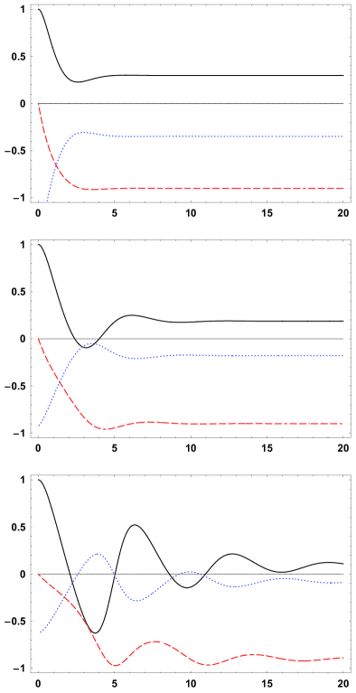
Figure 1: Profiles of $\left\langle\hat{\sigma}_{z}\right\rangle_{t}$ (solid line), $(\hbar\Omega)^{-1}\langle\hat{H}_{+}\rangle_{t}$ (dashed line), and $-(\hbar\Omega)^{-1}\langle\hat{\Gamma}\rangle_{t}$ (dotted line) versus $2\beta\Omega t$, for $\beta=0.9$, $a_{2}=0.01$ and, from top to bottom, $\gamma/\beta=1,0.5,0.2$.

Further, from the constraint in Eq. (39) it follows that, once $\gamma$ and $a_{2}$ are fixed, the oscillatory frequency is always bound from above by the critical value $\omega_{c}$. This latter is, in turn, bound from above by $\omega_{+}=2\Omega$, i.e., $\omega\leqslant\omega_{c}\leqslant\omega_{+}$, with $\omega_{c}=\beta_{c}\,\omega_{+}$, $\beta_{c}^{2}=1-(a_{2}^{2}/(\gamma^{2}+1))\leqslant\bar{\beta}^{2}$, and $\bar{\beta}=\pm 1$. This can be summarized by saying that at a given decay rate, the parameter $a_{2}$ measures the difference of the system’s critical frequency from the tunneling frequency of the Hermitian two-level system whose Hamiltonian is given in (36).

IV Evolution with conserved average energy

There are instances in which the coupling to the environment produces dissipation while leaving the average energy $\langle\hat{H}_{+}\rangle_{t}$ of the system constant. One such case is provided, for example, by the canonical ensemble. In order to describe the relaxation toward the constant average energy condition at large times, we impose

$$\lim\limits_{t\to+\infty}\langle\hat{\sigma}_{x}\rangle_{t}=-(\hbar\Omega)^{-1}\lim\limits_{t\to+\infty}\langle\hat{H}_{+}\rangle_{t}=0,$$ (54)

which is equivalent, according to (53), to the constraint

$$\beta=0.$$ (55)

It turns out that this condition leads to the coherence (34) in this case vanishes not just asymptotically but identically,

$$\langle\hat{\sigma}_{x}\rangle_{t}=-(\hbar\Omega)^{-1}\langle\hat{H}_{+}\rangle_{t}=0,$$ (56)

which can be shown by directly substituting (55) into (50). This model can be further cast into subclasses, depending on whether the parameter $a_{2}$ is chosen to be zero or not.

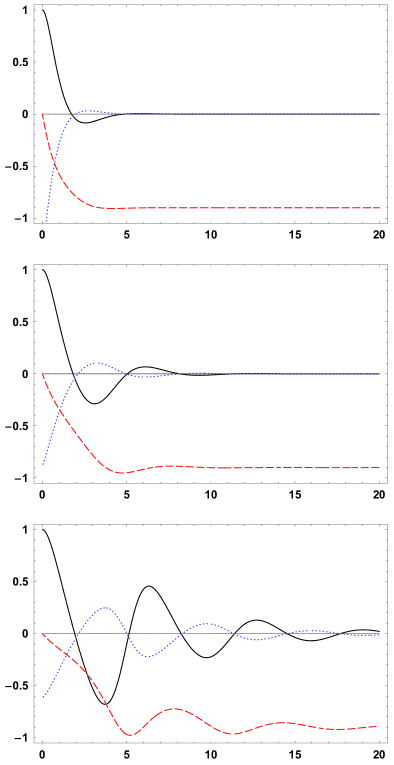
Figure 2: Profiles of the averages: $\left\langle\hat{\sigma}_{z}\right\rangle$ (solid line), $(\hbar\Omega)^{-1}\langle\hat{H}_{+}\rangle_{t}$ (dashed line) and $-(\hbar\Omega)^{-1}\langle\hat{\Gamma}\rangle_{t}$ (dotted line) versus time variable $2\beta\Omega t$, evaluated at $\beta=0.9$, constraint (76) and, from top to bottom, $\gamma/\beta=$ 1, 1/2, 1/5.

IV.1 Exponential decay of $\langle\sigma_{y}\rangle_{t}$ and $\langle\sigma_{z}\rangle_{t}$

By this we assume that the observables approach their asymptotic values exponentially fast. If we impose that $a_{2}\not=0$ then non-Hermitian Hamiltonian is defined by the sum of the Hermitian Hamiltonian in Eq. (36) and of the anti-Hermitian decay operator

$$\hat{\Gamma}^{\text{(ed)}}=\hbar\Omega\left(a_{2}\hat{\sigma}_{y}+\hat{\sigma}_{z}+\gamma\hat{I}\right)\;.$$ (57)

multiplied by the imaginary unit. In such a case, the evolution equation yield the following solution

$$\hat{\rho}_{11}(t)=\frac{1}{a_{2}^{2}}\left[a_{2}\cosh{(\alpha t/2)}-\sinh{(\alpha t/2)}\right]^{2}e^{-\Gamma t}\;,$$ (58)

$$\hat{\rho}_{12}(t)=-\hat{\rho}_{21}(t)=\frac{i}{2a_{2}^{2}}(a_{2}-1)\left[1-\cosh{(\alpha t)}+a_{2}\sinh{(\alpha t)}\right]e^{-\Gamma t}\;,$$ (59)

$$\hat{\rho}_{22}(t)=\frac{1}{a_{2}^{2}}(a_{2}-1)^{2}\sinh^{2}{(\alpha t/2)}e^{-\Gamma t}\;,$$ (60)

where $\alpha=2a_{2}\Omega$ and the decay rate coefficient $\Gamma$ was defined in (48). If we define

$$T^{(\text{ed})}(t)=(a_{2}^{2}-a_{2}+1)\cosh{(\alpha t)}-a_{2}\sinh{(\alpha t)}+a_{2}-1\;,$$ (61)

the trace of density operator can be written as

$$\text{tr}(\hat{\rho}(t))=\frac{1}{a_{2}^{2}}e^{-\Gamma t}T^{(\text{ed})}(t).$$ (62)

The analytical expressions of the averages of the spin operators do not depend on $\gamma$ (yet, their behavior depends on the sign of $\gamma$ which determines whether the exponents are decreasing or increasing with time); they are given below

$$\langle\hat{\sigma}_{x}\rangle_{t}=0\;,$$ (63)

$$\langle\hat{\sigma}_{y}\rangle_{t}=\frac{a_{2}-1}{T^{(\text{ed})}(t)}\left[\cosh{(\alpha t)}-a_{2}\sinh{(\alpha t)}-1\right],$$ (64)

$$\langle\hat{\sigma}_{z}\rangle_{t}=\frac{a_{2}}{T^{(\text{ed})}(t)}\left(a_{2}-1+e^{-\alpha t}\right).$$ (65)

The asymptotic behaviour of the above-mentioned quantities significantly depends on values of the parameters. If, for definiteness, one assumes throughout this section that

$$\gamma>0,$$ (66)

then one can find that the parametric space of $a_{2}$ has the following physically admissible domains:

(i) $0<a_{2}<\gamma$:
In this case the density matrix vanishes at large times. The asymptotic values of other observables become:

$$\lim\limits_{t\to+\infty}\langle\hat{\sigma}_{y}\rangle_{t}=-1,\ \lim\limits_{t\to+\infty}\langle\hat{\sigma}_{z}\rangle_{t}=0.$$ (67)

(ii) $0<-a_{2}<\gamma$:
In this case the density matrix also vanishes at large times, asymptotic values of other observables are given by:

$$\lim\limits_{t\to+\infty}\langle\hat{\sigma}_{y}\rangle_{t}=\frac{a_{2}^{2}-1}{a_{2}^{2}+1},\ \ \lim\limits_{t\to+\infty}\langle\hat{\sigma}_{z}\rangle_{t}=\frac{2a_{2}}{a_{2}^{2}+1}.$$ (68)

IV.2 Polynomial decay of $\langle\sigma_{y}\rangle_{t}$ and $\langle\sigma_{z}\rangle_{t}$

By this we assume that the observables approach their asymptotic values in a way which is described by a polynomial or rational function of time. This can be achieved by choosing the decay operator as

$$\hat{\Gamma}^{(\text{pd})}=\hbar\Omega\left(\hat{\sigma}_{z}+\gamma\hat{I}\right)\;.$$ (69)

The corresponding non-Hermitian Hamiltonian is obtained by adding (36) to this decay operator (being multiplied by the imaginary unit). Keeping the initial density matrix in the form of Eq. (43), the evolution equation is solved analytically. The matrix elements have the following explicit time dependence

$$\hat{\rho}_{11}(t)=(\Omega t-1)^{2}e^{-\Gamma t}\;,$$ (70)

$$\hat{\rho}_{12}(t)=-\hat{\rho}_{21}(t)=i\Omega t\left(\Omega t-1\right)e^{-\Gamma t}\;,$$ (71)

$$\hat{\rho}_{22}(t)=\Omega^{2}t^{2}e^{-\Gamma t}\;.$$ (72)

If we introduce $T^{(\text{pd})}(t)=2\Omega t(\Omega t-1)+1,$ the trace of density operator is given by

$$\text{tr}(\hat{\rho}(t))=e^{-\Gamma t}T^{(\text{pd})}(t)\;.$$ (73)

The analytical expressions of the averages of the Pauli operators are given in this case by

$$\langle\hat{\sigma}_{x}\rangle_{t}=0,\ \ \langle\hat{\sigma}_{y}\rangle_{t}=\frac{2\Omega t(1-\Omega t)}{T^{(\text{pd})}(t)},\ \ \langle\hat{\sigma}_{z}\rangle_{t}=\frac{1-2\Omega t}{T^{(\text{pd})}(t)},$$ (74)

and one can see that these observables evolve according to a polynomial law rather than exponential. Assuming that $\gamma>0$, the limit for $t\to\infty$ of the density matrix and of the averages $\langle\hat{\sigma}_{y}\rangle_{t}$ and $\langle\hat{\sigma}_{z}\rangle_{t}$ are $-1$ and $0$, respectively. This is similar to the case $a_{2}>0$ above, with the only difference being that these observables approach their asymptotic states not exponentially fast but in a polynomial time.

V Asymptotically vanishing population difference

For open systems one often expects that the population difference goes to zero at large times:

$$\lim\limits_{t\to+\infty}\langle\hat{\sigma}_{z}\rangle_{t}=0.$$ (75)

This is equivalent, according to (53), to the constraints

$$a_{2}-\gamma\sqrt{1-\beta^{2}}=0,\ \ W=\sqrt{1-\beta^{2}},$$ (76)

such that the anti-Hermitian part of the Hamiltonian (40) simplifies to

$$\hat{\Gamma}^{(\text{vp})}=-\hbar\gamma\Omega\left[\beta\hat{\sigma}_{x}-\sqrt{1-\beta^{2}}(\hat{\sigma}_{y}+\gamma^{-1}\hat{\sigma}_{z})-\hat{I}\right],$$ (77)

and the analytical expressions for a solution from the section III hold provided one makes changes in constants according to the constraints (76):

$$\hat{\rho}_{11}(t)=\frac{1}{2}\frac{e^{-\Gamma t}}{\beta^{2}+\gamma^{2}}\left[A_{8}\cos{(\omega t)}+\tilde{\gamma}^{2}\cosh{(\Gamma t)}-2W(\beta\sin{(\omega t)}+\gamma\sinh{(\Gamma t)})\right]\;,$$ (78)

$$\hat{\rho}_{12}(t)=\frac{1}{2}\frac{e^{-\Gamma t}}{\beta^{2}+\gamma^{2}}\left[A_{9}(\cos{(\omega t)}-\cosh{(\Gamma t)})+B_{5}(\sinh{(\Gamma t)}-i\sin{(\omega t)})\right],$$ (79)

$$\hat{\rho}_{22}(t)=\frac{1}{2}\frac{e^{-\Gamma t}}{\beta^{2}+\gamma^{2}}\left[(2\gamma W-\tilde{\gamma}^{2})(\cos{(\omega t)}-\cosh{(\Gamma t)})\right],$$ (80)

where we denoted

$$\tilde{\gamma}=\sqrt{1+\gamma^{2}},$$ (81)

and $A_{8}=\tilde{\gamma}^{2}-2W^{2}$, $A_{9}=W(\gamma\beta+i(\gamma W-1))$, $B_{5}=\beta(\tilde{\gamma}^{2}-\gamma W)+i\gamma W(\gamma-W))$ with $W$ being defined in (76).

The asymptotic values of observables become:

$$\lim\limits_{t\to+\infty}\langle\hat{\sigma}_{x}\rangle_{t}=-(\hbar\Omega)^{-1}\lim\limits_{t\to+\infty}\langle\hat{H}_{+}(t)\rangle=\beta,$$

$$\lim\limits_{t\to+\infty}\langle\hat{\sigma}_{y}\rangle_{t}=-\sqrt{1-\beta^{2}},$$ (82)

whereas the critical frequency saturates the upper bound, $\omega_{c}=\omega_{+}$ and $\beta_{c}^{2}=1$. We thus obtain

$$\beta^{2}\leqslant 1\ \Rightarrow\ \omega\leqslant\omega_{+},$$ (83)

the profiles of observables for this model are shown in Fig. 2.

VI Dephasing

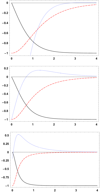
Figure 3: Profiles of the averages: $\left\langle\hat{\sigma}_{z}\right\rangle$ (solid line), $(\hbar\Omega)^{-1}\langle\hat{H}_{+}\rangle_{t}$ (dashed line) and $-(\hbar\Omega)^{-1}\langle\hat{\Gamma}\rangle_{t}$ (dotted line) versus time variable $2\gamma\Omega t$, evaluated at, from top to bottom, $\gamma=$ 4, 1, 1/5.

It can be interesting to investigate whether non-Hermitian dynamics can cause an initial non-diagonal density matrix to become diagonal at large times: this is known as the dephasing. To this end, let us choose at time zero the following density matrix

$$\hat{\rho}(0)=\frac{1}{2}\sum_{k,m=g,e}|k\rangle\langle m|=\left(\begin{array}[]{cc}1/2&~{}~{}1/2\\ 1/2&~{}~{}1/2\end{array}\right).$$ (84)

If the anti-Hermitian part of the Hamiltonian (40) is chosen as

$$\hat{\Gamma}^{(\text{dph})}=-\hbar\Omega\left[\hat{\sigma}_{y}-\gamma\left(\sigma_{z}+\hat{I}\right)\right],$$ (85)

then the evolution equation yields

$$\hat{\rho}_{11}(t)=\frac{1}{2}e^{-2\Gamma t}\;,$$ (86)

$$\hat{\rho}_{12}(t)=\hat{\rho}_{21}(t)^{*}=\frac{1}{2\gamma}e^{-2\Gamma t}\left[(\gamma-i)e^{\Gamma t}+i\right],$$ (87)

$$\hat{\rho}_{22}(t)=\frac{1}{2\gamma^{2}}\left[\left(e^{-\Gamma t}-1\right)^{2}+\gamma^{2}\right],$$ (88)

where the decay rate coefficient was defined in (48).

Further, the averages can be written as

$$\langle\hat{\sigma}_{x}\rangle_{t}=\frac{\gamma^{2}}{\tilde{\gamma}^{2}\cosh{(\Gamma t)}-1},$$ (89)

$$\langle\hat{\sigma}_{y}\rangle_{t}=\frac{\gamma(1-e^{-\Gamma t})}{\tilde{\gamma}^{2}\cosh{(\Gamma t)}-1},$$ (90)

$$\langle\hat{\sigma}_{z}\rangle_{t}=\frac{1-\cosh{(\Gamma t)}-\gamma^{2}\sinh{(\Gamma t)}}{\tilde{\gamma}^{2}\cosh{(\Gamma t)}-1},$$ (91)

where $\tilde{\gamma}$ was defined in (81). We thus obtain the following asymptotics

$$\lim\limits_{t\to+\infty}\hat{\rho}(t)=\frac{1}{2}\left(1+\gamma^{-2}\right)|g\rangle\langle g|\;,$$ (92)

$$\lim\limits_{t\to+\infty}\langle\hat{\sigma}_{x}\rangle_{t}=\lim\limits_{t\to+\infty}\langle\hat{\sigma}_{y}\rangle_{t}=0,$$ (93)

$$\lim\limits_{t\to+\infty}\langle\hat{\sigma}_{z}\rangle_{t}=-1.$$ (94)

The dephasing is accompanied by the certainty of occupying the ground state for $t\to\infty$. The evolution of the observables is shown in Fig. 3.

VII Mixed states and purification

The control over the purification of TLS quantum states is currently of great theoretical baker90 ; pur-th ; pur-th2 ; pur-th3 and experimental pur-exp ; pur-exp2 ; pur-exp3 interest since it is important for the quantum state engineering and quantum computation technology. In this section we consider the problem of the asymptotical purification of mixed states under non-Hermitian dynamics. Let us study the evolution of some generic mixed state and find out the conditions under which it purifies at large times. As an example, the Hamiltonian is chosen as a special case of the one given in (40),

$$\hat{H}=-\hbar\Omega\left[\hat{\sigma}_{x}+i\left(a_{2}\hat{\sigma}_{y}+W\hat{\sigma}_{z}+a_{0}\hat{I}\right)\right],$$ (95)

where $W=\sqrt{1+\gamma^{2}-a_{2}^{2}}$, and $a_{0}$, $a_{2}$ and $\gamma$ are free parameters. The anti-Hermitian part of this Hamiltonian is not the most general but it is sufficient for the main purpose of this section. As in previous sections, the value of $a_{0}$ does not enter expressions for the normalized density matrix and physical observables, and thus it can be left free or it can be chosen ad hoc, e.g., to make the non-normalized density matrix convergent, as it happens when one sets $a_{0}=\gamma>0$. Here we choose the initial condition

$$\hat{\rho}(0)=p|g\rangle\langle g|+(1-p)|e\rangle\langle e|=\left(\begin{array}[]{cc}1-p&~{}~{}0\\ 0&~{}~{}p\end{array}\right),$$ (96)

where $p$ is a constant parameter, $0<p<1$. Solving the equation of motion (3) with the Hamiltonian (95), we obtain

$$\hat{\rho}_{11}(t)=\Lambda(t)\left[(k_{1}(W)-2\gamma W)e^{2\Gamma t}-2(k_{1}(\gamma)-2\gamma^{2})e^{\Gamma t}+k_{1}(-W)+2\gamma W\right],$$

$$\hat{\rho}_{12}(t)=-\hat{\rho}_{21}(t)=i\Lambda(t)\left[\gamma(a_{2}+p_{1})(e^{2\Gamma t}-1)+W(a_{2}p_{1}+1)(e^{\Gamma t}-1)^{2}\right],$$ (97)

$$\hat{\rho}_{22}(t)=\Lambda(t)\left[k_{2}(-W)e^{2\Gamma t}+2a_{2}(p-1)(e^{\Gamma t}-1)^{2}-2k_{2}(\gamma)e^{\Gamma t}+k_{2}(W)\right],$$

and

$${\rm tr}\hat{\rho}(t)=2\Lambda(t)\left[p_{+}e^{2\Gamma t}+a_{2}p_{1}(e^{\Gamma t}-1)^{2}-2e^{\Gamma t}+p_{-}\right],$$ (98)

where we denoted

$$\Lambda(t)=(2\gamma)^{-2}e^{-\tilde{\Gamma}t},\ \tilde{\Gamma}=\Gamma+2a_{0}\Omega,$$

$$p_{1}=2p-1,\ p_{\pm}=\tilde{\gamma}^{2}\pm p_{1}\gamma W,$$

$$k_{1}(\eta)=\gamma^{2}+W^{2}+2p(1+a_{2}-W^{2}+\eta\gamma),$$

$$k_{2}(\eta)=\gamma^{2}-W^{2}-2p(1-W^{2}+\eta\gamma)+2,$$

and $\Gamma$ and $\tilde{\gamma}$ have been defined in (48) and (81), respectively.

The asymptotic behaviour of the density operator crucially depends on whether the initial-state parameter $p$ lies on the constraint surface

$$\Upsilon(p,a_{2},\gamma)\equiv p_{1}(a_{2}+\gamma W)+\tilde{\gamma}^{2}=0.$$ (99)

We distinguish the following two cases:

(i) Asymptotically pure states. For those initial states for which $\Upsilon(p,a_{2},\gamma)$ does not vanish at arbitrary $a_{2}$ and $\gamma$, the normalized density matrix (8) derived from the solution (97) has the following large-times asymptotics:

$$\hat{\rho}_{11}^{\prime}(+\infty)=\frac{1}{2\Upsilon(p,a_{2},\gamma)}\left[k_{1}(W)-2\gamma W\right],$$

$$\hat{\rho}_{12}^{\prime}(+\infty)=-\hat{\rho}_{21}^{\prime}(+\infty)=\frac{i}{2\Upsilon(p,a_{2},\gamma)}\left[\gamma(a_{2}+p_{1})+W(a_{2}p_{1}+1)\right],$$ (100)

$$\hat{\rho}_{22}^{\prime}(+\infty)=\frac{1}{2\Upsilon(p,a_{2},\gamma)}\left[k_{2}(-W)+2a_{2}(p-1)\right],$$

so one can check that

$$\lim\limits_{t\to+\infty}\det\hat{\rho}^{\prime}(t)=0,$$ (101)

at any non-singular values of the parameters $a_{2}$ and $\gamma$.

(ii) Asymptotically mixed states. For those initial states for which $\Upsilon(p,a_{2},\gamma)$ vanishes (which may happen if the parameters of anti-Hermitian part obey the inequality $\tilde{\gamma}^{2}<\left|a_{2}+\gamma W\right|$), one can derive the condition for an initial-state parameter:

$$p=\frac{1}{2}\frac{a_{2}+\gamma W-\tilde{\gamma}^{2}}{a_{2}+\gamma W}.$$ (102)

Under this condition the normalized density matrix derived from the solution (97) has the following large-times asymptotics:

$$\hat{\rho}_{11}^{\prime}(+\infty)=\frac{1}{2}\frac{(W-\gamma)(\tilde{\gamma}^{2}+a_{2}+\gamma W)}{W-a_{2}\gamma},$$

$$\hat{\rho}_{12}^{\prime}(+\infty)=-\hat{\rho}_{21}^{\prime}(+\infty)=\frac{1}{2}iW,$$ (103)

$$\hat{\rho}_{22}^{\prime}(+\infty)=\frac{1}{2}\frac{(W+\gamma)(\tilde{\gamma}^{2}-a_{2}-\gamma W)}{W-a_{2}\gamma},$$

so one obtains

$$\lim\limits_{t\to+\infty}\det\hat{\rho}^{\prime}(t)=\frac{\gamma^{2}}{4}\frac{W^{2}(\gamma^{2}-1)+2a_{2}\gamma W-(\gamma\tilde{\gamma})^{2}}{(W-a_{2}\gamma)^{2}},$$ (104)

which does not vanish for arbitrary values of the parameters of anti-Hermitian part.

To summarize, for the example considered in this section, the purification under non-Hermitian evolution can be controlled by an appropriate choice of the parameters appearing in the anti-Hermitian part of the Hamiltonian.

VIII Conclusion

In this paper we have considered a two-level system described by a Hermitian Hamiltonian and added an anti-Hermitian term to it. Hence, we have considered the dynamics resulting from the total non-Hermitian Hamiltonian. The anti-Hermitian part of the Hamiltonian has been assumed to effectively describe the averaged influence of degrees of freedom associated with the environment. This influence is encoded in the parameters of the anti-Hermitian part which can be tuned in order to implement desired properties into a model. We have also established that the value of the trace of anti-Hermitian part plays an important role in determining the decaying behaviour of the system (or absence thereof).

When analyzing the evolution of the total system, we have focused on the density matrix of the model and expressed observables through it. Analytical solutions have been obtained in a number of relevant cases - such as when the evolution takes place with dephasing or vanishing population difference. The various types of decays produced show that non-Hermitian dynamics is able to mimic the effects of an environment onto a two-level system. In the case of mixed-state evolution, we considered as an example a specific Hamiltonian and clarified the conditions under which the dynamics led to the purification of the initial state. One of the possible future directions would be to apply this formalism to those physical systems which allow the two-mode approximation.

References

• (1) N. Moiseyev, Non-Hermitian Quantum Mechanics (Cambridge University Press, Cambridge, 2011).
• (2) C. M. Bender, Rep. Prog. Phys. 70, 947 (2007).
• (3) B. D. Wibking and K. Varga, Phys. Lett. A 376 365 (2012).
• (4) K.-F. Berggreen, I. I. Yakimenko, and J. Hakanen, New. J. Phys. 12 073005 (2010).
• (5) M. Znojil, Phys. Rev. D 80 045009 (2009).
• (6) K. Varga and S. T. Pantelides, Phys. Rev. Lett. 98 076804 (2007).
• (7) J.G. Muga, J.P. Palao, B. Navarro, and I.L. Egusquiza, Phys. Rep. 395 357 (2004).
• (8) N. Moiseyev, Phys. Rep. 302 211 (1998).
• (9) W. John, B. Milek, H. Schanz, and P. Seba, Phys. Rev. Lett. 67 1949 (1991).
• (10) C. A. Nicolaides and S. I. Themelis Phys. Rev. A 45 349 (1992).
• (11) E. C. G. Sudarshan, Phys. Rev. D 18 2914 (1978).
• (12) S. Selstø, T. Birkeland, S. Kvaal, R. Nepstad, and M. Førre, J. Phys. B: At. Mol. Opt. Phys. 44 215003 (2011).
• (13) H. C. Baker, Phys. Rev. Lett. 50, 1579–1582 (1983).
• (14) H. C. Baker, Phys. Rev. A 30 773 (1984).
• (15) S.-I. Chu and W. P. Reinhardt, Phys. Rev. Lett. 39 1195 (1977).
• (16) C. E. Rüter, K. G. Makris, R. El-Ganainy, D. N. Christodoulides, M. Segev, and D. Kip, Nature Physics 6 192 (2010).
• (17) A. Guo, G. J. Salamo, D. Duchesne, R. Morandotti, M. Volatier-Ravat, V. Aimez, G. A. Siviloglou, and D. N. Christodoulides, Phys. Rev. Lett. 103 093902 (2009).
• (18) J. Wong, J. Math. Phys. 8, 2039 (1967).
• (19) G. C. Hegerfeldt, Phys. Rev. A 47, 449 (1993).
• (20) S. Baskoutas, A. Jannussis, R. Mignani, and V. Papatheou, J. Phys. A: Math. Gen. 26 L819 (1993).
• (21) P. Angelopoulou, S. Baskoutas, A. Jannussis, R. Mignani, and V. Papatheou, Int. J. Mod. Phys. B 9 2083 (1995).
• (22) I. Rotter, arXiv:0711.2926.
• (23) I. Rotter, J. Phys. A 42 153001 (2009).
• (24) H. B. Geyer, F. G. Scholtz and K. G. Zloshchastiev, in: Proceedings of $12^{\text{th}}$ International Conference on Mathematical Methods in Electromagnetic Theory (Odessa, 2008) 250-252.
• (25) R. Lo Franco, B. Bellomo, S. Maniscalco, and G. Compagno, Int. J. Mod. Phys. B 27 1345053 (2013).
• (26) S. Banerjee and R. Srikanth, Mod. Phys. Lett. B 24 2485 (2010).
• (27) F. Reiter and A. S. Sørensen, Phys. Rev. A 85 032111 (2012).
• (28) H. Feshbach, Ann. Phys. 5 357 (1958).
• (29) H. Feshbach, Ann. Phys. 19 287 (1962).
• (30) G. Dattoli, A. Torre, and R. Mignani, Phys. Rev. A 42 1467 (1990).
• (31) F. H. M. Faisal and J. V. Moloney, J. Phys. B: At. Mol. Opt. Phys. 14 3603 (1981).
• (32) A. Thilagam, J. Chem. Phys. 136 065104 (2011).
• (33) E.-M. Graefe and R. Schubert, Phys. Rev. A 83, 060101 (2011).
• (34) E.-M. Graefe, M. Höning, and H. J. Korsch, J. Phys. A 43 075306 (2010).
• (35) H.-P. Breuer and F. Petruccione, The Theory of Open Quantum Systems (Oxford University Press, Oxford, 2002).
• (36) J. A. Holyst and L. A. Turski, Phys. Rev. A 45 6180 (1992).
• (37) A. Sergi, Comm. Theor. Phys. 56 96 (2011).
• (38) N. Gisin, J. Phys. A 14 2259 (1981).
• (39) N. Gisin, Physica A 111, 364 (1982).
• (40) N. Gisin, J. Math. Phys. 24, 1779 (1983).
• (41) H. J. Korsch and H. Steffen, J. Phys. A 20 3787 (1987).
• (42) M. D. Kostin, J. Chem. Phys. 57 (1973) 3589.
• (43) M. D. Kostin, J. Stat. Phys. 12 (1975) 145.
• (44) I. Bialynicki-Birula and J. Mycielski, Annals Phys.  100, 62-93 (1976).
• (45) K. Yasue, Annals Phys.  114 (1978) 479.
• (46) N. A. Lemos, Phys. Lett. A 78 (1980) 239.
• (47) J. D. Brasher, Int. J. Theor. Phys. 30 (1991) 979.
• (48) D. Schuch, Phys. Rev. A 55, 935 (1997).
• (49) M. P. Davidson, Nuov. Cim. B 116 (2001) 1291.
• (50) J. L. Lopez, Phys. Rev. E. 69 (2004) 026110.
• (51) K. G. Zloshchastiev, Grav. Cosmol. 16 (2010) 288.
• (52) K. G. Zloshchastiev, Acta Phys. Polon. B 42 (2011) 261.
• (53) A. V. Avdeenkov and K. G. Zloshchastiev, J. Phys. B: At. Mol. Opt. Phys. 44 (2011) 195303.
• (54) E.-M. Graefe, H. J. Korsch, and A. E. Niederle, Phys. Rev. A 82, 013629 (2010).
• (55) C. Gerry and P. Knight, Introductory Quantum Optics (Cambridge University Press, Cambridge, 2005).
• (56) H. C. Baker and R. L. Singleton, Phys. Rev. A 42 10 (1990).
• (57) L. P. Hughston, R. Jozsa, and W. K. Wootters, Phys. Lett. A 183, 14 (1993).
• (58) A. Bassi and G. Ghirardi, Phys. Lett. A 309, 24 (2003).
• (59) M. Kleinmann, H. Kampermann, T. Meyer, and D. Bruss, Phys. Rev. A 73, 062309 (2006).
• (60) J.-W. Pan, S. Gasparoni, R. Ursin, G. Weihs, and A. Zeilinger, Nature (London) 423, 417 (2003).
• (61) Z. Zhao, T. Yang, Y.-A. Chen, A.-N. Zhang, and J.-W. Pan, Phys. Rev. Lett. 90, 207901 (2003).
• (62) A. E. B. Nielsen, C. A. Muschik, G. Giedke, and K. G. H. Vollbrecht, Phys. Rev. A 81, 043832 (2010).