Quasiclassical molecular dynamics for the dilute Fermi gas at unitarity

Abstract

We study the dilute Fermi gas at unitarity using molecular dynamics with an effective quantum potential constructed to reproduce the quantum two-body density matrix at unitarity. Results for the equation of state, the pair correlation function and the shear viscosity are presented. These quantities are well understood in the dilute, high temperature, limit. Using molecular dynamics we determine higher order corrections in the diluteness parameter $n\lambda^{3}$, where $n$ is the density and $\lambda$ is the thermal de Broglie wave length. In the case of the contact density, which parameterizes the short distance behavior of the correlation function, we find that the results of molecular dynamics interpolates between the truncated second and third order virial expansion, and are in excellent agreement with existing T-matrix calculations. For the shear viscosity we reproduce the expected scaling behavior at high temperature, $\eta\sim 1/\lambda^{3}$, and we determine the leading density dependent correction to this result.

I Introduction

There has been a significant amount of interest in equilibrium and transport properties of cold atomic quantum gases near a Feshbach resonance bloch2008 ; giorgini2008 ; Schafer:2009dj ; Adams:2012th . The Feshbach resonance is used to tune the energy of a molecular bound state to the threshold of a scattering state, causing the scattering length to diverge. At resonance the scattering cross-section is universal, independent of the microscopic details, and is limited only by unitarity. In this regime there are no small parameters that can be used to justify a perturbative expansion.

The only ab-initio approach to the problem is the quantum Monte-Carlo (QMC) method Carlson:2003zz ; Astrakharchik:2004zz ; Bulgac:2005pj ; Lee:2005it ; goulko2010 ; Drut:2011tf ; Endres:2012cw . QMC simulations have been used successfully to compute thermodynamic properties, but it is very difficult to use imaginary time QMC simulations to compute real-time response functions and transport coefficients (see, however, Wlazlowski:2012jb for a recent attempt). This implies that we lack reliable bench mark calculations for experimental attempts to determine the viscosity of a degenerate Fermi gas near unitarity. While the viscosity can be computed reliably at both high Massignan:2005zz ; Bruun:2006kj ; Bruun:2005en and low Rupak:2007vp ; Mannarelli:2012su temperature there is no systematic approach in the strongly coupled regime $T\sim T_{F}$, where $T_{F}$ is the Fermi temperature. A number of authors have used diagrammatic methods to study transport properties in this regime Enss:2010qh ; Guo:2011 , but it is not a priori clear what kind of diagrams have to be included.

In this work we introduce a novel approach to the dynamics of quantum gases. The method is based on a classical molecular dynamics simulation in which quantum effects are encoded in an effective classical interaction among the atoms. The quasi-classical $N$-body interaction is constructed such that the classical calculation exactly reproduces the diagonal component of the quantum $N$-body density matrix. This implies, in particular, that the $N$’th quantum virial coefficient is reproduced. In this paper we restrict ourselves to two-body terms in the interaction. In this case the second virial coefficient will be reproduced exactly, and through molecular dynamic simulations, the one and two-body components of the higher virial coefficients are resumed. The strength of the molecular dynamics method is that very complicated many body correlations are taken into account. The drawback is that genuine quantum many-body effects such as pairing and superfluidity are not included. Quasi-classical molecular dynamics has been used successfully in the study of strongly correlated Coulomb plasmas Golubnychiy:2001 ; Bonitz:2003 . However, our work differs in that the quasi-classical potential for unitary fermions is of purely quantum mechanical origin. In contrast, the quasi-classical Coulomb potential, known as the Kelbg potential Kelbg:1963 , is a small correction to the classical $1/r$ behavior. Quasi-classical methods were also used by Feynman and Kleinert to study the high temperature limit of the partition function for simple quantum systems Feynman:1986ey .

This paper is organized as follows. In Sect. II and III we introduce the method and derive the quasi-classical potential at unitarity. In Sect. IV we describe the molecular dynamics simulations and in Sect. V we present results for the equation of state, the pair correlation function, and the shear viscosity.

II The partition function

In this section we introduce a classical partition function which is equivalent, order-by-order in a cluster expansion, to the full quantum partition function. The classical partition function depends on $k$-body potentials which can be determined from the quantum mechanical Slater sums. In this work we will restrict ourselves to the case $k=2$, which means that the second virial coefficient is reproduced exactly. We will follow the notation used in huang1987statistical .

The quantum mechanical partition function for a system of $N$ particles is given by

$$\mathcal{Z}_{N}=\frac{1}{N!\lambda^{3N}}\int\left(d{\bf r}_{1}\ldots d{\bf r}_{N}\right)W^{(N)}\left({\bf r}_{1},\ldots,{\bf r}_{N}\right)\,,$$ (1)

where we have defined the $N$-particle Slater sums

$$W^{(N)}\left({\bf r}_{1},\ldots,{\bf r}_{N}\right)=N!\lambda^{3N}\sum_{\alpha}|\Psi_{\alpha}\left({\bf r}_{1},\ldots,{\bf r}_{N}\right)|^{2}e^{-\beta E_{\alpha}}\,.$$ (2)

In this expression $\lambda=\sqrt{\frac{2\pi\hbar^{2}}{mk_{B}T}}$ is the thermal wavelength, $\beta=1/T$ is the inverse temperature, and $\Psi_{\alpha}({\bf r}_{1},\ldots,{\bf r}_{N})$ is the wave function of an $N$ particle state with energy $E_{\alpha}$. The partition function can be expanded systematically in powers of $n\lambda^{3}$ in terms of the virial coefficients $b_{l}$,

$$\mathcal{Z}_{N}=\sum_{\{m_{l}\}}\prod_{l=1}^{N}\frac{1}{m_{l}!}\left(\frac{V}{\lambda^{3}}b_{l}\right)^{m_{l}}\,,$$ (3)

where $\{m_{l}\}$ is a set of integers $m_{l}\geq 0$ that satisfies the constraint $\sum_{l=1}^{N}lm_{l}=N$. The corresponding expression for the pressure has the form

$$\frac{P}{kT}=\frac{1}{\lambda^{3}}\sum_{l=1}^{\infty}b_{l}z^{l}\,,$$ (4)

where $z=e^{\beta\mu}$ is the fugacity and $\mu$ is the chemical potential. Each virial coefficient $b_{N}$ can be expressed in terms of integrals over the $N$-particle Slater sums. For example

$$b_{2} =\frac{1}{2!\lambda^{3}V}\int d{\bf r}_{1}d{\bf r}_{2}\left[W^{(2)}({\bf r}_{1},{\bf r}_{2})-W^{(1)}({\bf r}_{1})W^{(1)}({\bf r}_{2})\right]\;,$$ (5)

$$b_{3} =\frac{1}{3!\lambda^{6}V}\int d{\bf r}_{1}d{\bf r}_{2}d{\bf r}_{3}\left[W^{(3)}({\bf r}_{1},{\bf r}_{2},{\bf r}_{3})-W^{(2)}({\bf r}_{1},{\bf r}_{2})W^{(1)}({\bf r}_{3})\right.$$

$$-\left.W^{(2)}({\bf r}_{2},{\bf r}_{3})W^{(1)}({\bf r}_{1})-W^{(2)}({\bf r}_{3},{\bf r}_{1})W^{(1)}({\bf r}_{2})+2W^{(1)}({\bf r}_{1})W^{(1)}({\bf r}_{2})W^{(1)}({\bf r}_{3})\right]\,.$$ (6)

We may compare these results to the corresponding expressions for a classical system. We consider the most general partition function containing arbitrary $N$-body interactions

$$\mathcal{Z}_{N}=\frac{1}{N!\lambda^{3N}}\int\left(d{\bf r}_{1},\ldots,d{\bf r}_{N}\right)e^{-\beta\sum_{i<j}v_{ij}-\beta\sum_{i<j<k}v_{ijk}+\cdots}\;.$$ (7)

The virial expansion of the classical partition function has the same form as the quantum expansion in Eq. (3), but the expressions for the virial coefficients are different. We have

$$b_{2} =\frac{1}{2!\lambda^{3}V}\int d{\bf r}_{1}d{\bf r}_{2}\left[e^{-\beta v_{12}}-1\right]\;,$$ (8)

$$b_{3} =\frac{1}{3!\lambda^{6}V}\int d{\bf r}_{1}d{\bf r}_{2}d{\bf r}_{3}\left[e^{-\beta\left(v_{123}+v_{12}+v_{23}+v_{13}\right)}-e^{-\beta v_{12}}-e^{-\beta v_{23}}-e^{-\beta v_{13}}+2\right]\;.$$ (9)

It is clear that one can construct a classical $N$-body potential so that the classical and quantum virial coefficients agree order by order. For example, we can construct effective 2 and 3-body potentials

$$v_{ij} =-\beta^{-1}\log\left(W^{(2)}\left({\bf r}_{i},{\bf r}_{j}\right)\right)\,,$$ (10)

$$v_{ijk} =-\beta^{-1}\log\frac{W^{(3)}({\bf r}_{1},{\bf r}_{2},{\bf r}_{3})}{W^{(2)}({\bf r}_{1},{\bf r}_{2})W^{(2)}({\bf r}_{2},{\bf r}_{3})W^{(2)}({\bf r}_{3},{\bf r}_{1})}\,,$$ (11)

such that the classical system described by the partition function in Eq. (7) will have the same virial coefficients as the quantum mechanical system at the same order. In practice we will truncate the expansion at second order. We note that even in this case we retain all contributions to the third and higher virial coefficients that arise from powers of $W^{(2)}$. Only genuine three and higher-body correlations are missing.

III Quasi-classical two-body potential at unitarity

As discussed in the previous section the first non-trivial virial coefficient can be reproduced by introducing the effective two-body potential defined in Eq. (10). The potential depends on the logarithm of the two-particle Slater sum $W^{(2)}$. This quantity is defined in terms of the solutions of the two-particle Schrödinger equation

$$\mathcal{H}\Psi_{\alpha}\left({\bf r}_{1},{\bf r}_{2}\right)=E_{\alpha}\Psi_{\alpha}\left({\bf r}_{1},{\bf r}_{2}\right)\,,$$

$$\mathcal{H}=-\frac{\hbar^{2}}{2m}\left({\bf\nabla}_{r_{1}}^{2}+{\bf\nabla}_{r_{2}}^{2}\right)+V\left(|{\bf r}_{1}-{\bf r}_{2}|\right)\;.$$ (12)

In the case of a spherically symmetric interaction the two particle Slater sum is only a function of the relative coordinate $r=|{\bf r}_{2}-{\bf r}_{1}|$. We find

$$W^{(2)}\left({\bf r}\right)=2^{5/2}\lambda^{3}\sum_{l}\frac{(2l+1)}{4\pi}\sum_{k}\;R_{kl}(r)^{2}e^{-\beta\epsilon_{k}}\;,$$ (13)

where $R_{kl}(r)$ satisfies the radial Schrödinger equation

$$\left[\frac{\partial^{2}}{\partial r^{2}}+\frac{2}{r}\frac{\partial}{\partial r}+\left(k^{2}-\frac{l(l+1)}{r^{2}}-V(r)\right)\right]R_{kl}(r)=0,\;\;\;\;\;\;k^{2}\equiv\frac{m}{\hbar^{2}}\epsilon_{k}\;.$$ (14)

III.1 Free particle

It is instructive to begin by deriving the effective classical potential for a free particle. This potential takes into account the effects of quantum statistics: repulsion for identical fermions, or attraction for identical bosons. The wave function of a free particle is

$$R_{kl}(r)=\sqrt{2k^{2}}j_{l}(kr)\;,$$ (15)

and the corresponding two-particle Slater sum is

$$W^{(2)}\left({\bf r}\right)=2^{7/2}\lambda^{3}\sum_{l}\frac{(2l+1)}{4\pi^{2}}\int k^{2}dk\;j_{l}(kr)^{2}e^{-\frac{\lambda^{2}k^{2}}{2\pi}}\;.$$ (16)

We compute the Slater sum for identical bosons and fermions by restricting the sum over all states to $l=\textrm{even}$ or $l=\textrm{odd}$, respectively. We find

$$W^{(2)}\left({\bf r}\right)=\frac{2^{1/2}\lambda^{3}}{\pi^{2}}\int dk\;k^{2}\;\left[1\pm\textrm{sinc}(2kr)\right]e^{-\frac{\lambda^{2}k^{2}}{2\pi}}=1\pm e^{-\frac{2\pi r^{2}}{\lambda^{2}}}\;,$$ (17)

where $\textrm{sinc}(x)=\textrm{sin}(x)/x$ and we have made use of the identities

$$\sum_{l=0,2,4,...}(2l+1)j^{2}_{l}(kr) =\frac{1+\textrm{sinc}(2kr)}{2}\,,$$

$$\sum_{l=1,3,5,...}(2l+1)j^{2}_{l}(kr) =\frac{1-\textrm{sinc}(2kr)}{2}\,.$$ (18)

The resulting potentials are therefore

$$u_{eff}^{\textrm{ideal}}=-k_{B}T\log\left(1\pm e^{-2\pi r^{2}/\lambda^{2}}\right)\,,$$ (19)

with the ‘+’ sign for bosons and the ‘-’ sign for fermions.

III.2 Classical potential at unitarity

At unitarity the physics is independent of the precise form of the interaction potential. We will therefore treat the interaction among opposite spin particles as arising from an attractive square well of depth $V_{0}$ and range $b$. In the zero range limit only $s$-wave scattering contributes to the scattering amplitude. Outside the range of the potential the $l=0$ wave function has the form

$$R_{k,l=0}=\sqrt{2k^{2}}\,\frac{\sin(kr+\delta_{0})}{kr}\;,$$ (20)

where $\delta_{0}$ is the $s$-wave phase shift. The correction to the free $l=0$ Slater sum is given by

$$\Delta W^{(2)}_{l=0}=\frac{\lambda^{3}}{\sqrt{2}r^{2}}\int dk\,\left[\sin^{2}\left(kr+\delta_{0}(k)\right)-\sin^{2}(kr)\right]e^{-\frac{\lambda^{2}k^{2}}{2\pi}}\,.$$ (21)

In principle analogous expressions can be found inside the interaction region $r<b$. However, at unitarity, we are interested in the limit $b\to 0$ while keeping $\sqrt{V_{0}}b=\pi/2$ fixed. We can therefore evaluate Eq. (21) for $\delta_{0}=\pi/2$ independent of $k$. In this case the integral is straightforward. We find

$$\Delta W^{(2)}_{l=0}=\frac{2\lambda^{2}}{\pi r^{2}}e^{-2\pi r^{2}/\lambda^{2}}\;,$$ (22)

and the effective potential at unitarity is given by

$$u_{eff}^{a\to\infty}=-k_{B}T\log\left(1+\frac{\lambda^{2}}{\pi r^{2}}e^{-2\pi r^{2}/\lambda^{2}}\right)\;.$$ (23)

We observe that the only length scale in the potential is the thermal wave length.

IV Molecular dynamics simulation

Having constructed the quasi-classical effective potential we now describe the molecular dynamics simulations. We consider a two component system with $N=N_{\uparrow}+N_{\downarrow}$ particles. The net polarization is zero and $N_{\uparrow}=N_{\downarrow}=N/2$. Using Eq. (19) and (23) the two body interactions between like and unlike spins are

$$u_{\uparrow\downarrow} =u_{\downarrow\uparrow}=-k_{B}T\log\Big{(}1+\frac{\lambda^{2}}{\pi r^{2}}e^{-2\pi r^{2}/\lambda^{2}}\Big{)}\,,$$

$$u_{\uparrow\uparrow} =u_{\downarrow\downarrow}=-k_{B}T\log\Big{(}1-e^{-2\pi r^{2}/\lambda^{2}}\Big{)}\,.$$ (24)

The molecular dynamics equations of motion are

$$\frac{d\vec{q}_{i}}{dt}=\frac{\vec{p}_{i}}{m}\,,\hskip 28.45274pt\frac{d\vec{p}_{i}}{dt}=\vec{F}_{i}\,,$$ (25)

where $i=1,\ldots,N$ and $F_{i}$ is the force on the $i$’th particle due to the potential given in Eq. (24). We measure the temperature in the simulation from the average kinetic energy per particle,

$$k_{B}T=\frac{1}{3N}\left\langle\sum_{i}m\left(\frac{d}{dt}\vec{r}_{i}\right)^{2}\right\rangle\,,$$ (26)

where the angular brackets denote an average over the simulation time. The pressure is computed using the virial theorem

$$PV=Nk_{B}T+\frac{1}{3}\left\langle\sum_{i}\vec{r}_{i}\cdot\vec{F}_{i}\right\rangle\,.$$ (27)

It is advantageous to adopt a system of dimensionless units in which to perform the molecular dynamics simulations. We have used the system of units described in Table 1. In particular, we use the thermal wave length $\lambda$ as the unit of distance, and $\lambda(m/T)^{1/2}$ as the unit of time. We will denote quantities that are expressed in simulation units by a star, for example $r^{*}=r/\lambda$. In this system of units the simulation temperature $T^{*}$ is equal to unity, and the physical temperature is adjusted by changing the density $n^{*}=n\lambda^{3}$. The ratio $T/T_{F}$, where $T_{F}=(3\pi^{2}n)^{2/3}\hbar^{2}/(2mk_{B})$ is the Fermi temperature, is given by $T/T_{F}=4\pi(3\pi^{2}n^{*})^{-2/3}$.

Simulation Units
Mass	$m=$ mass of one atom
Length	$\lambda$
Energy	$k_{B}\times$system temperature
Time	$t^{*}=\lambda\sqrt{m/T}$
Derived Units
density	$n^{*}=N\lambda^{3}/V$
Temperature	$T^{*}=1$
Pressure	$P^{*}=P\lambda^{3}/T$
Shear viscosity	$\eta^{*}=\eta\lambda^{3}/Tt^{*}$

Table 1: System of units used in the numerical simulations of this work.

We note that the effective quasi-classical potential is temperature dependent. In practice we choose a simulation density $n^{*}=n\lambda^{3}$. We initialize the simulation using a guess for the total kinetic energy. We monitor the kinetic energy as the system equilibrates and add or subtract energy by rescaling the velocities to reach the desired simulation temperature $T^{*}=1$. After the system equilibrates at this temperature we measure observables like the equation of state, the pair correlation function, and the correlation function of the stress tensor. The main simulation parameters are listed in Table 2. Fluctuations are used to determine statistical errors. In addition, there are a number of systematic errors whose effect are difficult to quantify. One such systematic error is due to the finite number of particles. For the equation of state we have performed calculations with $N=32$, $N=108$ and $N=256$ particles. Fig. 1 shows that the corresponding results agree within the statistical errors. Due to computational limitations we have only used runs with $N=108$ for our calculations of the pair and stress tensor correlation functions. Another source of systematic uncertainty is the fact that molecular dynamics simulations are most naturally performed in a microcanonical ensemble (at fixed energy). This requires us to tune the energy very precisely in order to reach the simulation temperature. This is challenging because of long equilibration times and finite size fluctuations.

Simulation Parameters
$N_{\textrm{atoms}}$	108
$l_{0}^{*}$	0.05
$\Delta t^{*}$	0.001
$t^{*}_{\textrm{equilibration}}$	2500
$t^{*}_{\textrm{thermostat}}$	50
$t^{*}_{\textrm{production}}$	$2\times 10^{5}$

Table 2: Parameters used in the numerical simulations of this work. $N_{\textrm{atoms}}$ is the number of atoms, $l_{0}^{*}$ is the cutoff in the potential, $\Delta t^{*}$ is the molecular dynamics time step, $t^{*}_{\textrm{equilibration}}$ is the equilibration time, $t^{*}_{\textrm{thermostat}}$ is the time between velocity rescalings during equilibration, and $t^{*}_{\textrm{production}}$ is the total length of the molecular dynamics trajectory. We have also performed runs with $N_{\textrm{atoms}}=32$ and $256$.

V Results

V.1 Equation of state

In this section we present our results for the equation of state. We also make comparisons to the available experimental data and to analytical results in the high temperature limit. The pressure in the limit $n\lambda^{3}\ll 1$ is given by the virial expansion

$$\frac{P}{nT}\simeq 1-b_{2}\left(\frac{n\lambda^{3}}{2}\right)+\left(4b_{2}^{2}-2b_{3}\right)\left(\frac{n\lambda^{3}}{2}\right)^{2}+O((n\lambda^{3})^{3})\,.$$ (28)

The second virial coefficient is well-known Beth:1936 ; Ho:2004zza , $b_{2}=3/(4\sqrt{2})$, and the third virial coefficient has been computed in PhysRevLett.98.090403 ; PhysRevLett.102.160401 ; Kaplan:2011br , $b_{3}=−0.29095295$.

In Fig. 1 we show the pressure normalized to $nT$ as a function of the dimensionless density $n\lambda^{3}$ and the temperature in units of the Fermi temperature, $T/T_{F}$. The data points show the results of the molecular dynamics simulations. The results are compared to the virial expansion at second and third order (dotted and dashed lines), and to a parameterization (band) of the experimental data from nascimbene2009eos . More accurate results for the equation of state have recently been published by the MIT group Ku:2011 . In the range of temperatures that are of interest to us, $T/T_{F}\gtrsim 0.5$, the more recent data agrees with the earlier data within the errors indicated by the thickness of the band.

We observe that the data follow the second order virial expansion for $n\lambda^{3}\mathrel{\hbox to0.0pt{\lower 4.0pt\hbox{\hskip 1.0pt$\sim$}\hss}\raise 1.0pt\hbox{$<$}}0.2$. This agreement is of course a consequence of the way the potential was constructed, but it serves as a useful check of the molecular dynamics (MD) simulation. We also observe that the full MD simulation is better behaved than the virial expansion. While the virial expansion is not useful for $n\lambda^{3}\gtrsim 0.3$ the MD results follow the data up to densities $n\lambda^{3}\sim(0.5-1.0)$. Assessing whether this improvement is fortuitous, or whether two-body interactions resummed by the MD simulation do indeed capture a significant part of the higher virial coefficients will require an explicit calculation of the three-body effective interaction, which we hope to pursue in a future work. The MD results do not reproduce the rapid increase in the pressure for $n\lambda^{3}\gtrsim 2$. Based on the sign of the third virial coefficient it is reasonable to assume that the MD results in this regime could be improved by including a repulsive three body potential.

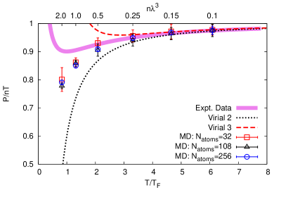
Figure 1: Pressure in units of the ideal gas pressure as a function of $T/T_{F}$ (bottom axis) and $n\lambda^{3}$ (top axis). The data were obtained from quasi-classical molecular dynamics simulations with different numbers of particles in a periodic box. The dashed and dotted lines show the virial expansion at second and third order, and the band is a parameterization of the experimental data of the ENS group nascimbene2009eos .

V.2 Pair correlation function

For a homogeneous system the pair correlation function is defined as

$$G(r,t)=\frac{V}{N\left(N-1\right)}\left<\sum_{i}\sum_{j\neq i}\delta\left[r-|\vec{r}_{i}(0)-\vec{r}_{j}(t)|\;\right]\right>\,.$$ (29)

The pair correlation function measures the probability of finding two particles separated by a distance $r$ and time $t$. For $t=0$ the quantity $G(r,0)$ is also known as the radial distribution function, or as the Fourier transform of the static structure factor. For a two component system we can define two correlation functions, $G_{\uparrow\uparrow}=G_{\downarrow\downarrow}$ and $G_{\uparrow\downarrow}=G_{\downarrow\uparrow}$, which characterize the probability of finding two particles of the same or opposite spin close to one another.

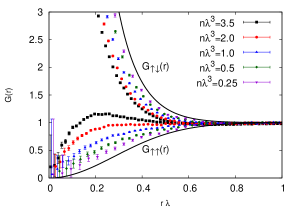
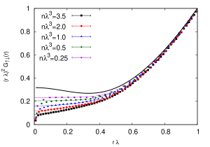
Figure 2: Radial distribution functions $G_{\uparrow\uparrow}$ and $G_{\uparrow\downarrow}$ extracted from molecular dynamics simulations with 108 particles performed at different values of the diluteness parameter $n\lambda^{3}$. The solid lines show the analytic result in the high temperature (low density) limit. The right panel shows the pair correlation function for unlike spins scaled by $r^{2}$. The intercept is proportional to Tan’s contact density ${\cal C}$. Note that the correlation function for $r\lambda<0.05$ is sensitive to the regulator in the potential. The thin solid lines show the fit described in the text.

Fig. 2 shows the radial distribution function for a system of 108 particles ($N_{\uparrow}=N_{\downarrow}=54$) at different densities. The solid curves show the high temperature ($n\lambda^{3}\ll 1$) limit

$$G(r,0)=\exp\left[-\frac{u_{eff}(r)}{k_{B}T}\right]\,,$$ (30)

where $u_{eff}$ is given in Eq. (24). We observe that the like spin correlation function is repulsive, which is a reflection of the Pauli principle, and the unlike spin correlation function is strongly attractive, which is a consequence of the attractive interaction in the spin singlet channel. The range of the correlation function is equal to the thermal wave length. The MD results show that at non-asymptotic temperatures the correlation function are more short range. We also observe that the equal spin correlation becomes attractive at intermediate range, and that there is less attraction in the opposite spin channel. The pair correlation function at zero temperature was studied using Green Function Monte Carlo (GFMC) Astrakharchik:2004zz ; Lobo:2006 . At $T=0$ the pair correlation function has the same shape as in the high temperature limit, but the range is set by $k_{F}^{-1}$.

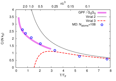
Figure 3: Contact density ${\cal C}$ in units of $Nk_{F}$ as a function of $n\lambda^{3}$ and $T/T_{F}$. We also show the high temperature limit from the virial expansion at second and third order, and the result of two T-matrix approximations, labeled GPF/G₀G₀ (see text).

The right panel of Fig. 2 shows the short distance behavior of the unlike spin correlation function. Tan observed that the correlation function is proportional to $1/r^{2}$ at all temperatures Tan:2008a ; Tan:2008b . The $1/r^{2}$ term is governed by a universal parameter known as Tan’s contact density ${\cal C}$,

$$G_{\uparrow\downarrow}(r,0)=\frac{\mathcal{C}}{16\pi^{2}n_{\downarrow}n_{\uparrow}}\left(\frac{1}{r^{2}}-\frac{2}{ar}\right)\,.$$ (31)

This relation combined with Eq. (30) shows that the contact density scales as $T^{-1}$ in the high temperature limit Yu:2009 ; Braaten:2010 ; Hu:2010 ,

$${\cal C}=\frac{32\pi^{2}n_{\downarrow}n_{\uparrow}}{mT}\,.$$ (32)

Fig. 2 shows that at non-asymptotic temperatures the contact is smaller than the limiting form given in Eq. (32). The pair correlation function in the limit $r\to 0$ is sensitive to the regulator $l_{0}$ in the potential. In order to extract the contact density we fit the unlike-spin correlation functions at short distances ($l_{0}\leq r\lambda\leq 0.5$) with the functional form $(r\lambda)^{2}G_{\uparrow\downarrow}(r\lambda)={\cal C}/(4\pi^{2}n^{2})+a_{0}(r\lambda)^{p}$, where $a_{0},p$ and ${\cal C}$ are treated as fit parameters. The quality of the fit can be seen from the thin solid lines in the right plot of Fig. 2. The value of the contact density obtained from the fit is shown in Fig. 3. The size of the data points approximate the error in the fitted contact density estimated by varying the size of the fit region by $10\%$ in either direction.

In Fig. 3 we also compare the MD result for the contact density to recent T-matrix calculations. The line labeled GPF/G₀G₀ shows the results for two particular truncations, the Generalized Pair Fluctuation (GPF) theory of Noziéres and Schmitt-Rink nsr ; Hu:2010 , and the non-self consistent (G₀G₀) T-matrix approximation of Palestini et al. Palestini:2010 . We find very good agreement between the results of the MD simulation and the T-matrix calculations for all densities we have studied, $0.05\mathrel{\hbox to0.0pt{\lower 4.0pt\hbox{\hskip 1.0pt$\sim$}\hss}\raise 1.0pt\hbox{$<$}}n\lambda^{3}\mathrel{\hbox to0.0pt{\lower 4.0pt\hbox{\hskip 1.0pt$\sim$}\hss}\raise 1.0pt\hbox{$<$}}2$. We also note that the T-matrix calculations (convoluted with suitable density profiles for finite traps) were shown to agree with the recent data reported in finiteTSwinExpt , see Hu:2010 .

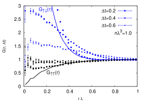
Figure 4: Unequal time pair correlation function for $n\lambda^{3}=1.0$ (left) and $n\lambda^{3}=3.5$ (right) at $\Delta t=0.2,0.4,0.6$, where $\Delta t$ is expressed in units of $\lambda\sqrt{m/T}$. The solid curves show the corresponding $\Delta t=0$ result from Fig. 2.

Fig. 4 shows the pair distribution function at non-zero time difference. This is the first quantity in this work that is not directly amenable to quantum Monte Carlo studies. The Fourier transform of $G(r,t)$ yields the dynamic structure function, which has been studied extensively in a variety of many-body theories bloch2008 ; giorgini2008 . We have not attempted to perform the Fourier transform, since this would require high statistics data on a very fine mesh. We observe that the typical correlation time in our data is of order one in simulation units $\lambda\sqrt{m/T}$.

VI Shear Viscosity

We compute the shear viscosity coefficient using the Green-Kubo relation

$$\eta_{(xy)} =\frac{V}{k_{B}T}\int_{0}^{\infty}\left\langle P_{xy}(t)P_{xy}(0)\right\rangle dt\;,$$ (33)

where $P_{xy}(t)$ is the stress energy tensor evaluated at time $t$ Haile:1992:MDS:531139 ; Rapaport:2004 ,

$$P_{xy}(t)=m\sum_{i=1}^{N}\dot{x}_{i}\dot{y}_{i}+\frac{1}{2}\sum_{i=1}^{N}\sum_{j\neq i}^{N}\frac{1}{r}\frac{\partial u_{ij}}{\partial r}\left(x_{i}-x_{j}\right)\left(y_{i}-y_{j}\right)\;.$$ (34)

There are five independent stress tensor correlation functions that can be used to determine the shear viscosity. We denote the corresponding estimates by $\eta_{(xy)},\eta_{(yz)},\eta_{(xz)},\eta_{(xxyy)}$ and $\eta_{(yyzz)}$, and use the average of the five measurements as our final result. The results for $N=108$ and $N=256$ is shown in Fig. 5.

We can check the MD simulation by comparing the numerical result to the expected behavior in the high temperature limit. The calculation of the transport cross section and the shear viscosity is explained in the Appendix. For a two component system with the classical interaction given in Eq. (24) the high temperature limit of the shear viscosity is

$$\left.\frac{\eta}{\hbar n}\right|_{\textrm{cl}}=\frac{75\sqrt{2}\pi}{8\left(5+\pi\right)n\lambda^{3}}\;.$$ (35)

This result is shown as the high temperature limit of the solid black line label ‘MD Fit’ in Fig. 5, and we observe that the agreement with the MD results in the regime $n\lambda^{3}\lesssim 0.15$ is very good. The classical result is about 20% larger than the (almost exact) quantum result in the high temperature limit Massignan:2005zz ; Bruun:2006kj ; Bruun:2005en

$$\frac{\eta}{\hbar n}=\frac{45\pi^{3/2}}{64\sqrt{2}}\left(\frac{T}{T_{F}}\right)^{3/2}=\frac{15\sqrt{2}\pi}{16(n\lambda^{3})}\;.$$ (36)

This result is shown as the dashed blue line in Fig. 5. The discrepancy between the classical and quantum calculation is due to a combination of two effects, discussed in more detail in Appendix A. The first is the fact that the unlike spin potential does not exactly reproduce the quantum mechanical transport cross section. The second effect is that the like spin potential, related to Pauli repulsion, leads to a finite transport cross section, even though there is no scattering in a quantum system of like spins interacting by a pure $s$-wave potential.

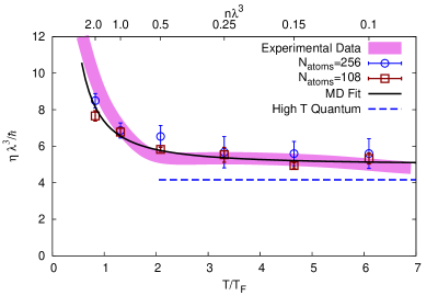
Figure 5: Molecular dynamics results for the shear viscosity $\eta$ in units of $\hbar\lambda^{-3}$ as a function of $n\lambda^{3}$ and $T/T_{F}$. The solid black line shows the fit to the MD results as described in the text, and the dashed blue line shows the quantum mechanical high temperature result. The band shows the experimental data published in Cao:2010wa ; Cao:2011fh . Note that the data represent trap averages, and that we have used the ideal gas temperature at the center of the trap.

Fig. 5 also shows a parameterization of the viscosity measured in Cao:2010wa ; Cao:2011fh . The thickness of the band approximates the statistical errors in the measurement. Note that the measured viscosity is a trap averaged quantity, and as a result there is a $\sim 20\%$ discrepancy between the data and the theoretical result in the high temperature limit (dashed line). The very close agreement between the measured viscosity and the MD simulations is therefore somewhat of a coincidence.

We note that the molecular dynamics simulation reproduces the $\lambda^{-3}$ scaling of the shear viscosity. We also emphasize that the numerical discrepancy between the classical and quantum result is quite small. It is therefore reasonable to extract an estimate of the leading density dependence of the shear viscosity from the MD simulation. We have fit the MD results shown in Fig. 5 with the expression

$$\eta=\frac{\eta_{0}}{\lambda^{3}}\left(1+c_{2}\left(n\lambda^{3}\right)\right)\;,$$ (37)

where $\eta_{0}$ was fixed using Eq. (35). We find $c_{2}\simeq 0.32$. The fit well represents the MD results in the density range studied in this work, $0.1\leq(n\lambda)^{3}\leq 2$, including the rise in $\eta/\lambda^{3}$ around $(n\lambda)^{3}\sim(0.5-2.0)$, which is also seen in the experimental data.

VII Discussion and future work

We have presented a new method for studying the dynamics of cold atomic gases based on molecular dynamics simulations with an effective quantum potential. In this work we have restricted ourselves to two-body interactions. In this case the MD simulation exactly reproduces the second virial coefficient and the pair correlation function in the dilute limit. We have measured the equation of state, the pair correlation function, and the shear viscosity for a range of densities $0.1\lesssim n\lambda^{3}\lesssim 2.0$. We find that we can reproduce the experimentally measured equation of state for densities $n\lambda^{3}\lesssim(0.5-1.0)$. This is an improvement over the virial expansion, which breaks down $n\lambda^{3}\gtrsim 0.3$, and we expect that the range of applicability can be extended by including a three-body force.

We have also measured the static and dynamic pair correlation functions as well as the shear viscosity. We find that in the dilute limit the contact ${\cal C}$ scales as $n_{\uparrow}n_{\downarrow}/(mT)$, in agreement with the prediction in Yu:2009 ; Hu:2010 . Higher order correlations suppress the contact relative to the asymptotic behavior. Excellent agreement between the MD simulations and T-matrix calculations is seen for $n\lambda^{3}\lesssim 2$.

In this regime the temperature dependence of the shear viscosity is well described by the functional form $\eta=\eta_{0}\lambda^{-3}(1+c_{2}n\lambda^{3})$. The scaling of $\eta$ with $\lambda^{-3}$ agrees with the expected behavior at unitarity. The parameter $\eta_{0}$ differs from the exact quantum mechanical behavior at high temperature by a factor 1.2. We discuss the origin of this factor in the appendix, but it would clearly be desirable to understand the physical origin of the discrepancy more clearly, and to investigate whether there are any improvements of the quasiclassical MD method that reproduce the correct transport cross section. The main result of the MD simulation is that the density dependence of the shear viscosity is weak, $c_{2}\simeq 0.32$, and that it tends to increase the shear viscosity.

There are a number of additional applications or further extensions of the work presented here:

1. BEC-BCS crossover: In this work we focused on a dilute Fermi gas at unitarity. Clearly, the same methods can be used to determine the effective potential and the leading $n\lambda^{3}$ correction to pair correlation functions and transport coefficients for the full BEC-BCS crossover.

2. Three-body forces: The method discussed in this work can be systematically improved by including $n$-body forces ($n\geq 3$). In the case of three-body forces this appears quite tractable. The three-particle Slater sum can be computed in hyper-spherical coordinates, and molecular dynamics with three-body interactions is computationally feasible.

3. Other transport coefficients: The methods used in this work can also be used to measure other transport properties like the spin diffusion constant studied theoretically in Bruun:2011 and recently measured by the MIT group sommer2011uni , or the thermal conductivity Braby:2010ec . It would be interesting to determined whether $n\lambda^{3}$ corrections are universal. It is also interesting to determine the bulk viscosity as one goes away from the unitary limit $a\to\infty$. At unitarity the bulk viscosity is expected to vanish based on theoretical reasons Son:2005tj , and existing experiments are consistent with these arguments Dusling:2011dq .

4. Lower dimensional systems: Recently Vogt et al. measured the shear viscosity of a two-dimensional Fermi gas Vogt:2011 . In two dimensions fluctuations are expected to be more important than in three dimensional systems. These effects are difficult to include in kinetic theory, but are automatically included in molecular dynamics.

Appendix A Shear viscosity of dilute classical and quantum gases

In this appendix we summarize the calculation of the shear viscosity for a dilute classical gas interacting via the potentials given in Eq. (24). This result provides an important check for the calculation of the viscosity using the Green-Kubo formula. For both quantum and classical gases the calculation of the shear viscosity using the Chapman-Enskog method ChapmanCowling yields

$$\eta=\frac{5}{8}\frac{\sqrt{\pi mk_{B}T}}{\overline{\sigma}_{\textrm{tr}}}\,,$$ (38)

where $\overline{\sigma}_{\textrm{tr}}$ is the energy averaged transport cross section

$$\overline{\sigma}_{\textrm{tr}}=\int_{0}^{\infty}\gamma^{7}e^{-\gamma^{2}}\;\sigma_{\textrm{tr}}\left(\gamma\right)\;d\gamma\,,$$ (39)

and $\sigma_{\textrm{tr}}\left(\gamma\right)$ is the transport cross section. The parameter $\gamma=\sqrt{E/k_{B}T}$ is the dimensionless relative velocity of the two-particle system. The calculation of the transport cross section is different in the classical and quantum case, both because the cross section is represented in a different way, and because of the presence of symmetry factors in the quantum mechanical calculation.

A.1 Dilute classical gas

In the classical case the cross section is computed from classical trajectories in the potential. We can write $\sigma_{\textrm{tr}}\left(\gamma\right)$ as a one dimensional integral over the impact parameter $b$

$$\sigma_{\textrm{tr}}\left(\gamma\right)=2\pi\int_{0}^{\infty}\left[1-\cos^{2}\chi\left(b,E\right)\right]b\;db\,.$$ (40)

In this expression the scattering angle $\chi(b,E)$ is a function of the impact parameter and of the kinetic energy in the center-of-mass system through the relation

$$\chi(b,E)=\pi-2b\int_{r_{0}(b,E)}^{\infty}\frac{r^{2}}{1-b^{2}/r^{2}-U(r)/E}\,,$$ (41)

where $U(r)$ is the interaction potential and $r_{0}$ is the distance of closest approach. The parameter $r_{0}$ is determined by the solution of

$$1-b^{2}/r_{0}^{2}-U(r_{0})/E=0\;.$$ (42)

For the potentials of interest, Eq. (24), all of the above expressions must be evaluated numerically. We find the following results for a two particles interacting through the $u_{\uparrow\downarrow}$ and $u_{\uparrow\uparrow}$ potentials,

$$\overline{\sigma}_{\textrm{tr}}^{\uparrow\downarrow} =\frac{2}{3}\lambda^{2}\times(1.004)\,,$$ (43)

$$\overline{\sigma}_{\textrm{tr}}^{\uparrow\uparrow} =\frac{2\pi}{15}\lambda^{2}\times\,(1.0006)\,,$$ (44)

where the factors 1.004 and 1.006 are the results of numerical integrals. This work studies a two-component gas with equal numbers of spin up and down particles. In the dilute limit this system can be treated as a classical mixture and the effective transport cross section is the average of the $\sigma_{\textrm{tr}}^{\uparrow\downarrow}$ and $\sigma_{\textrm{tr}}^{\uparrow\uparrow}$ cross sections. The shear viscosity is

$$\left.\frac{\eta}{\hbar n}\right|_{\textrm{cl}}=\frac{75\sqrt{2}\pi}{8\left(5+\pi\right)n\lambda^{3}}\,,$$ (45)

which agrees with the high temperature MD simulation as shown in Fig. 5.

A.2 Dilute quantum gas

The quantum mechanical cross section can be represented in terms of the scattering phase shifts. In quantum mechanics we also have to take into account the symmetry of the wave function, which depends on whether the particles are distinguishable or not. For distinguishable particles the transport cross section is ChapmanCowling

$$\sigma_{\textrm{tr}}\left(\gamma\right)=\frac{4\pi}{k^{2}}\sum_{l}\frac{(l+1)(l+2)}{(2l+3)}\sin^{2}\left[\delta_{l+2}(k)-\delta_{l}(k)\right]\,,$$ (46)

where $k\equiv\sqrt{mE}/\hbar$ with $E$ the center of mass energy. The parameter $\gamma$ is given by $\gamma\equiv\sqrt{E/k_{B}T}$ as above. For indistinguishable particles

$$\sigma_{\textrm{tr}}\left(\gamma\right)=\frac{8\pi}{k^{2}}\sum_{l=\textrm{e/o}}\frac{(l+1)(l+2)}{(2l+3)}\sin^{2}\left[\delta_{l+2}(k)-\delta_{l}(k)\right]\,,$$ (47)

where the sum is restricted to even/odd (e/o) angular momenta for bosons/fermions. For a two-component Fermi gas interacting via an $s$-wave interaction we can treat the collisions between atoms of opposite spin as occurring between distinguishable particles. At unitarity the transport cross section is

$$\sigma^{\uparrow\downarrow}_{\textrm{tr}}(\gamma)=\frac{8\pi}{3k^{2}}\,,$$ (48)

and the energy averaged cross section is given by

$$\overline{\sigma}_{\textrm{tr}}^{\uparrow\downarrow}=\frac{4}{3}\lambda^{2}\;.$$ (49)

We find that the quantum cross-section is a factor of two larger than the analogous classical cross-section, Eq. (43). As in the classical case, the effective transport cross-section entering into the viscosity consists of an average over the $\sigma^{\uparrow\downarrow}$ and $\sigma^{\uparrow\uparrow}$ channels. As the latter is zero the overall cross-section is reduced by a factor of two. The final result is

$$\frac{\eta}{\hbar n}=\frac{15\sqrt{2}\pi}{16(n\lambda^{3})}\;.$$ (50)

References

- (1) I. Bloch, J. Dalibard, and W. Zwerger. Many-body physics with ultracold gases. Rev. Mod. Phys. 80:885 (2008).
- (2) S. Giorgini, L. P. Pitaevskii, and S. Stringari. Theory of ultracold atomic Fermi gases. Rev. Mod. Phys. 80:1215 (2008).
- (3) T. Schäfer and D. Teaney. Nearly Perfect Fluidity: From Cold Atomic Gases to Hot Quark Gluon Plasmas. Rep. Prog. Phys. 72:126001 (2009).
- (4) A. Adams, L. D. Carr, T. Schäfer, P. Steinberg and J. E. Thomas, Strongly Correlated Quantum Fluids: Ultracold Quantum Gases, Quantum Chromodynamic Plasmas, and Holographic Duality, arXiv:1205.5180 [hep-th].
- (5) J. Carlson, S. -Y. Chang, V. R. Pandharipande and K. E. Schmidt. Superfluid Fermi Gases with Large Scattering Length. Phys. Rev. Lett. 91, 050401 (2003).
- (6) G. E. Astrakharchik, J. Boronat, J. Casulleras and S. Giorgini. Equation of State of a Fermi Gas in the BEC-BCS Crossover: A Quantum Monte Carlo Study. Phys. Rev. Lett. 93, 200404 (2004).
- (7) A. Bulgac, J. E. Drut and P. Magierski, Spin 1/2 Fermions on a 3D-Lattice in the Unitary Regime at Finite Temperatures. Phys. Rev. Lett. 96, 090404 (2006) [cond-mat/0505374].
- (8) D. Lee and T. Schäfer. Cold dilute neutron matter on the lattice. II. Results in the unitary limit. Phys. Rev. C 73, 015202 (2006) [nucl-th/0509018].
- (9) Olga Goulko and Matthew Wingate. Thermodynamics of balanced and slightly spin-imbalanced fermi gases at unitarity. Phys. Rev. A, 82:053621, Nov 2010.
- (10) J. E. Drut, T. A. Lahde, G. Wlazlowski and P. Magierski. The Equation of State of the Unitary Fermi Gas: An Update on Lattice Calculations. arXiv:1111.5079 [cond-mat.quant-gas].
- (11) M. G. Endres, D. B. Kaplan, J. -W. Lee and A. N. Nicholson. Lattice Monte Carlo calculations for unitary fermions in a finite box. arXiv:1203.3169 [hep-lat].
- (12) G. Wlazlowski, P. Magierski and J. E. Drut. Shear Viscosity of a Unitary Fermi Gas. arXiv:1204.0270 [cond-mat.quant-gas].
- (13) P. Massignan, G. M. Bruun, and H. Smith. Viscous relaxation and collective oscillations in a trapped Fermi gas near the unitarity limit. Phys. Rev. A71:033607 (2005).
- (14) G. M. Bruun and H. Smith. Shear viscosity and damping for a Fermi gas in the unitarity limit. Phys. Rev. A75:043612 (2007).
- (15) G. M. Bruun and H. Smith. Viscosity and thermal relaxation for a resonantly interacting Fermi gas. Phys. Rev. A72:043605 (2005).
- (16) G. Rupak and T. Schäfer. Shear viscosity of a superfluid Fermi gas in the unitarity limit. Phys. Rev. A76:053607 (2007) [arXiv:0707.1520 [cond-mat.other]].
- (17) M. Mannarelli, C. Manuel, and L. Tolos. Shear viscosity in a superfluid cold Fermi gas at unitarity. arXiv:1201.4006 [cond-mat.quant-gas].
- (18) T. Enss, R. Haussmann, and W. Zwerger, Viscosity and scale invariance in the unitary Fermi gas. Annals Phys. 326, 770-796 (2011). [arXiv:1008.0007 [cond-mat.quant-gas]].
- (19) H. Guo, D. Wulin, C.-C. Chien, and K. Levin, Microscopic Approach to Shear Viscosities of Unitary Fermi Gases above and below the Superfluid Transition. Phys. Rev. Lett. 107, 020403 (2011).
- (20) V. Golubnychiy, M. Bonitz, D. Kremp, and M. Schlanges. Dynamical properties and plasmon dispersion of a weakly degenerate correlated one-component plasma. Phys. Rev. E 64, 016409 (2001).
- (21) M. Bonitz, D. Semkat, A. Filinov, V. Golubnychyi, D. Kremp, D. O. Gericke, M. S. Murillo, V. Filinov, V. E. Fortov, W. Hoyer, and S. W. Koch, Theory and Simulation of Strong Correlations in Quantum Coulomb Systems. J. Phys. A: Math. Gen. 36, 5921-5930 (2003).
- (22) G. Kelbg, Theorie des Quanten-Plasmas. Annalen der Physik 467, 219 (1963).
- (23) R. P. Feynman and H. Kleinert, Effective Classical Partition Functions. Phys. Rev. A 34, 5080 (1986).
- (24) K. Huang. Statistical mechanics. Wiley (1987).
- (25) G. E. Uhlenbeck, E. Beth. The quantum theory of the non-ideal gas I. Deviations from the classical theory. Physica 3, 729 (1936).
- (26) T.-L. Ho, E. J. Mueller. High temperature expansion applied to fermions near Feshbach resonance. Phys. Rev. Lett. 92 160404 (2004) [arXiv:cond-mat/0306187].
- (27) G. Rupak. Universality in a 2-component fermi system at finite temperature. Phys. Rev. Lett. 98:090403 (2007).
- (28) X.-J. Liu, H. Hu, and P. D. Drummond. Virial expansion for a strongly correlated fermi gas. Phys. Rev. Lett. 102:160401 (2009).
- (29) D. B. Kaplan and S. Sun, A New field theoretic method for the virial expansion, Phys. Rev. Lett. 107, 030601 (2011) [arXiv:1105.0028 [cond-mat.stat-mech]].
- (30) T. Schäfer. Dissipative fluid dynamics for the dilute Fermi gas at unitarity: Free expansion and rotation. Phys. Rev. A82:063629 (2010) [arXiv:1008.3876 [cond-mat.quant-gas]].
- (31) S. Nascimbène, N. Navon, KJ Jiang, F. Chevy, and C. Salomon. Exploring the thermodynamics of a universal Fermi gas. Nature, 463(7284):1057 (2010).
- (32) M. J. H. Ku, A. T. Sommer, L. W. Cheuk, and M. W. Zwierlein, Revealing the Superfluid Lambda Transition in the Universal Thermodynamics of a Unitary Fermi Gas. Science 335, 563 (2012) [arXiv:1110.3309 [cond-mat.quant-gas]].
- (33) C. Lobo, I. Carusotto, S. Giorgini, A. Recati, and S. Stringari. Pair correlations of an expanding superfluid fermi gas. Phys. Rev. Lett. 97:100405 (2006).
- (34) S. Tan. Energetics of a strongly correlated Fermi gas. Annals of Physics 323 2952 (2008) [arXiv:cond-mat/0505200].
- (35) S. Tan. Large momentum part of a strongly correlated Fermi gas. Annals of Physics 323 2971 (2008) [arXiv:cond-mat/0508320].
- (36) Z. Yu, G. M. Bruun, G. Baym. Short-range correlations and entropy in ultracold atomic Fermi gases. Phys. Rev. A 80, 023615 (2009) [arXiv:0905.1836 [cond-mat.quant-gas]]
- (37) E. Braaten, Universal Relations for Fermions with Large Scattering Length. Lect. Notes Phys. 836 193 (2012) [arXiv:1008.2922 [cond-mat.quant-gas]].
- (38) H. Hu, X.-J. Liu, P. D. Drummond. Universal contact of strongly interacting fermions at finite temperatures. New J. Phys. 13, 035007 (2011) [arXiv:1011.3845 [cond-mat.quant-gas]].
- (39) P. Noziéres and S. Schmitt-Rink. Bose condensation in an attractive fermion gas: From weak to strong coupling superconductivity. J. Low Temp. Phys. 59, 195 (1985).
- (40) M. Punk and W. Zwerger. Theory of rf-Spectroscopy of Strongly Interacting Fermions. Phys. Rev. Lett. 99, 170404 (2007) [arXiv:0707.0792 [cond-mat.other]]
- (41) J. E. Drut, T. A. Lahde and T. Ten. Momentum Distribution and Contact of the Unitary Fermi gas. Phys. Rev. Lett. 106, 205302 (2011) [arXiv:1012.5474 [cond-mat.stat-mech]].
- (42) F. Palestini, A. Perali, P. Pieri, and G. C. Strinati. Phys. Rev. A 82, 021605(R) (2010) [arXiv:1005.1158 [cond-mat.quant-gas]].
- (43) E. D. Kuhnle, S. Hoinka, P. Dyke, H. Hu, P. Hannaford, C. J. Vale. Temperature dependence of the contact in a unitary Fermi gas. Phys. Rev. Lett. 106, 170402 (2011) [arXiv:1012.2626].
- (44) J. M. Haile. Molecular Dynamics Simulation: Elementary Methods. John Wiley & Sons, Inc., New York, NY, USA, 1st edition (1992).
- (45) D. C. Rapaport. The Art of Molecular Dynamics Simulation. Cambridge University Press (2004).
- (46) C. Cao, E. Elliott, J. Joseph, H. Wu, J. Petricka, T. Schäfer and J. E. Thomas, Universal Quantum Viscosity in a Unitary Fermi Gas. Science, 331:58 (2011).
- (47) C. Cao, E. Elliott, H. Wu and J. E. Thomas, New J. Phys. 13 (2011) 075007 [arXiv:1105.2496 [cond-mat.quant-gas]].
- (48) G. M. Bruun. Spin diffusion in fermi gases. New Journal of Physics, 13(3):035005 (2011).
- (49) A. Sommer, M. Ku, G. Roati, and M. W. Zwierlein. Universal spin transport in a strongly interacting fermi gas. Nature, 472(7342):201-4 (2011).
- (50) M. Braby, J. Chao and T. Schäfer, Thermal Conductivity and Sound Attenuation in Dilute Atomic Fermi Gases. Phys. Rev. A 82, 033619 (2010) [arXiv:1003.2601 [cond-mat.quant-gas]].
- (51) D. T. Son, Vanishing bulk viscosities and conformal invariance of unitary Fermi gas. Phys. Rev. Lett. 98, 020604 (2007) [cond-mat/0511721].
- (52) K. Dusling and T. Schäfer. Elliptic flow of the dilute Fermi gas: From kinetics to hydrodynamics. Phys. Rev. A84:013622 (2011) [arXiv:1103.4869 [cond-mat.stat-mech]].
- (53) E. Vogt, M. Feld, B. Fröhlich, D. Pertot, M. Koschorreck, M. Köhl. Scale invariance and viscosity of a two-dimensional Fermi gas. Phys. Rev. Lett. 108, 070404 (2012) [arXiv:1111.1173 [cond-mat.quant-gas]].
- (54) S. Chapman and T. Cowling. Mathematical Theory of Non-uniform Gases (1970).