Memristive properties of single-molecule magnets

Abstract

Single-molecule magnets weakly coupled to two ferromagnetic leads act as memory devices in electronic circuits—their response depends on history, not just on the instantaneous applied voltage. We show that magnetic anisotropy introduces a wide separation of time scales between fast and slow relaxation processes in the system, which leads to a pronounced memory dependence in a wide intermediate time regime. We study the response to a harmonically varying bias voltage from slow to rapid driving within a master-equation approach. The system is not purely memristive but shows a partially capacitive response on short time scales. In the intermediate time regime, the molecular spin can be used as the state variable in a two-terminal molecular memory device.

I Introduction

Electronic transport through magnetic molecules has been extensively studied both experimentallyPPG02 ; LSB02 ; HGF06 ; JGB06 ; JRB07 ; GTT08 ; IRH08 ; SKC09 ; ZBO10 ; RVE11 ; KIL11 ; MKR11 ; MGD12 and theoretically.ElT05 ; RWS06 ; LeM06 ; TiE06 ; ElT06 ; LeL07 ; MiB07a ; GoL07 ; CUB07 ; JIM08 ; RLW09 ; LZS09 ; MWB09 ; ElT10 ; SoC10 ; JCG10 ; Yu10 ; CRA11 ; MWB11 ; LEK12 ; BAL12 The magnetic moment of these molecules can be realized by one or more transition-metal ions with organic ligands, by organic radicals, or by endohedral fullerenes. Transition-metal ions in a molecular ligand field typically show sizable magnetic anisotropy. In the case of a pronounced easy axis, one then speaks of single-molecule magnets (SMMs). For memory devices, easy-axis anisotropy is desirable since it introduces an energy barrier for spin reversal and thereby stabilizes the spin in the up or down orientation.TiE06

Driving the system with an external electric field allows the control and manipulation of the molecular spin state, and consequently writing and reading of information using SMMs.TiE06 Clearly, the response of the system to the applied electric field is not purely instantaneous—the system has memory. This can be compared to the response of SMMs to a magnetic field. At low temperatures, they show pronounced hysteresis in the magnetization (of bulk crystals of noninteracting SMMs) vs the magnetic field.SGC93 ; FrS10

Similarly, if a harmonically varying bias voltage is applied, we expect hysteresis loops in the spin, charge, and current dynamics vs the applied voltage to develop, whose amplitude depends on the voltage amplitude and frequency—as in other systems whose spin polarization can be controlled by a voltage or current; see, e.g., Ref. pershin08a, . At very low frequencies, the spin dynamics can easily follow the external field and little or no hysteresis is expected. At very high frequencies, the spin dynamics are “frozen.” There is, however, an intermediate frequency range—comparable to the inverse spin-relaxation time(s)—where the hysteresis is most pronounced. In this range, the device state, at any given time, is strongly dependent on the history of states through which the system has evolved. In that case, we expect the resistance of the device to be a function of the state variable $x$ that describes its memory (the spin polarization) and possibly of the protocol with which the voltage $V(t)$ has been applied, i.e., the entire wave form of $V(t)$. In other words, the resistive response can be characterized by a function of the type $R(x,V,t)$. Such a device goes under the name of memristive (for “memory resistive”) system.chua76a ; diventra09a ; PeV11 Resistors with memory are experiencing a surge of research activity, in part due to promising applications in memory storage, but also because of their ubiquity in diverse areas ranging from nontraditional computing to biophysics.pershin09b ; pershin10c ; pershin12a It is natural to think that SMMs form another example of memristive systems, with the molecular spin playing the role of internal state variable. This would have the added advantage of combining memristive and spintronics functionalitypershin08a ; wang2009 in molecular junctions. Indeed, Miyamachi et al.MGD12 have recently demonstrated memristive behavior of single $\mathrm{Fe}(1,10-\mathrm{phenanthroline})_{2}(\mathrm{NCS})_{2}$ molecules on CuN under a scanning tunneling microscope. In their case, the molecule is switched between a high-spin ($S=2$) and a low-spin ($S=0$) state of the $\mathrm{Fe}^{2+}$ ion, which is connected with a change in conformation and conductance. Our case is quite different: We consider the switching of a molecular local spin of fixed length $S$ over an anisotropy barrier.

In this paper, we show that the response of this system is only partially memristive. In addition, capacitive components emerge on short time scales. The capacitive components are related to the charging energy of the molecule and thus to the Coulomb repulsion of electrons.

Transport through magnetic molecules is typically dominated by a strong exchange interaction between the spin of mobile electrons and the local molecular spin, in addition to the large Coulomb repulsion. We are thus faced with a strongly interacting nonequilibrium system, which makes a quantitative description difficult in general. However, if the coupling between the molecule and the metallic leads is weak, as is often the case in break junctions, this coupling can be used as the small parameter in a perturbative approach. This can be done in the framework of the master equation, which has the advantage that the strong interactions within the molecule can be treated exactly. The master equation has been applied to transport through magnetic molecules by various groups.ElT05 ; RWS06 ; TiE06 ; ElT06 ; LeL07 ; MiB07a ; GoL07 ; JIM08 ; RLW09 ; LZS09 ; MWB09 ; ElT10 ; SoC10 It provides an ensemble description, not a description of individual time series of single-molecule devices. Statements we make about the memristive properties are thus to be understood in an ensemble sense. On the other hand, devices consisting of a monolayer of weakly interacting molecules between metallic electrodes, in which many molecules conduct in parallel, are self-averaging. In this case, we predict the time-dependent observables of a single device.

The analysis of SMMs as memory devices requires us to study their dynamics under a time-dependent bias. In Refs. TiE06, and ElT06, , their relaxation for constant or suddenly switched bias has been considered. Here, we consider the current, charge, and spin response to a harmonically varying bias $V(t)=V_{0}\,\sin\omega t$, which is easily realizable experimentally. For a non-magnetic molecule involving a vibrational mode, the response to a harmonic voltage has been recently studied by Donarini et al.DYG12 In this case, Franck-Condon blockade leads to interesting dynamics.Koch ; DYG12

The remainder of this paper is organized as follows: In Sec. II we present our model, followed by a discussion of the master-equation approach in Sec. III. The results are presented and discussed in Sec. IV. Finally, in Sec. V we summarize the main points, address possible limiting effects, and draw some conclusions.

II Model

Our device consists of a magnetic molecule coupled to two ferromagnetic leads. The full system is described by the Hamiltonian $H=H_{\mathrm{mol}}+H_{\mathrm{leads}}+H_{\mathrm{hyb}}$, where the molecular Hamiltonian readsTiE06 ; ElT06 ; MiB07a

$$H_{\mathrm{mol}}=\epsilon_{d}\sum_{\sigma}d^{\dagger}_{\sigma}d_{\sigma}+Ud^{\dagger}_{\uparrow}d_{\uparrow}d^{\dagger}_{\downarrow}d_{\downarrow}-J\mathbf{s}\cdot\mathbf{S}-K_{2}\,(S^{z})^{2},$$ (1)

where $d^{\dagger}_{\sigma}$ ($d_{\sigma}$) creates (annihilates) an electron of spin $\sigma$ in the molecular orbital with energy $\epsilon_{d}$, $\mathbf{s}\equiv\sum_{\sigma\sigma^{\prime}}d^{\dagger}_{\sigma}(\mbox{\boldmath$\sigma$}_{\sigma\sigma^{\prime}}/2)d_{\sigma}$ is the corresponding spin operator, and $\mathbf{S}$ is the spin operator of a local spin of length $S$. The two spins are coupled by the exchange interaction $J$ and the local spin is subject to an easy-axis anisotropy of strength $K_{2}>0$. The extension of this model by including more than one electronic orbital, or more than one local spin, does not pose any conceptual difficulties. In a break-junction setup, the on-site energy $\epsilon_{d}$ could be tuned by a gate voltage. However, this tunability is not necessary for our conclusions.

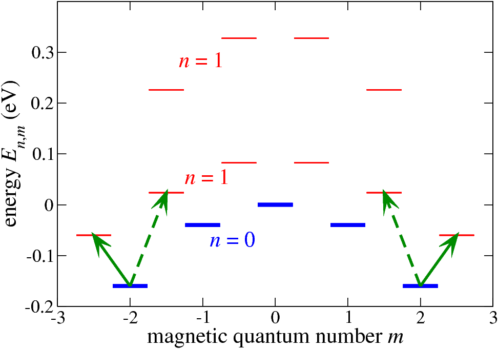
Figure 1: (Color online) Molecular energy levels $E_{n,m}$ vs magnetic quantum number $m$ for $\epsilon_{d}=0.2\,\mathrm{eV}$, $U=10\,\mathrm{eV}$, $J=0.1\,\mathrm{eV}$, $K_{2}=40\,\mathrm{meV}$, and $S=2$. Levels for electron occupation number $n=0$ ($n=1$) are shown as heavy blue (medium red) bars. Levels for electron number $n=2$ are outside the range of the plot. The arrows indicate the lowest-energy sequential-tunneling transitions out of the ground states.

The molecular Hamiltonian $H_{\mathrm{mol}}$ commutes with the z component of the total spin $\mathbf{S}_{\mathrm{tot}}\equiv\mathbf{s}+\mathbf{S}$ so that the eigenvalue $m$ of $S_{\mathrm{tot}}^{z}$ is a good quantum number. We show in Fig. 1 the energy levels of $H_{\mathrm{mol}}$ vs $m$ for the parameter values $\epsilon_{d}=0.2\,\mathrm{eV}$, $U=10\,\mathrm{eV}$, $J=0.1\,\mathrm{eV}$, $K_{2}=40\,\mathrm{meV}$, and $S=2$, which we will also use below to illustrate our results. Note that we are using a large value of the anisotropy energy in order to most clearly show the generic behavior. For the smaller anisotropies of SMMs,FrS10 the interesting physics would occur in a narrower voltage range and at lower temperatures. For $n=0$ and for $n=2$ electrons on the molecule, the total spin is just given by the local spin $\mathbf{S}$ so that there are $2S+1$ levels in these charge sectors. For one electron, $n=1$, its spin $1/2$ combines with the local spin $S$ to form two multiplets of $2(S-1/2)+1=2S$ and $2(S+1/2)+1=2S+2$ states. The splitting between the two multiplets is on the order of $JS$. The easy-axis anisotropy leads to the parabolic dispersion seen for all multiplets in Fig. 1. The total dimension of the molecular Fock space is $N_{F}=4(2S+1)$.

The leads are described by the Hamiltonian

$$H_{\mathrm{leads}}=\sum_{\nu\mathbf{k}\sigma}\epsilon_{\nu\mathbf{k}\sigma}\,c^{\dagger}_{\nu\mathbf{k}\sigma}c_{\nu\mathbf{k}\sigma},$$ (2)

where $c^{\dagger}_{\nu\mathbf{k}\sigma}$ ($c_{\nu\mathbf{k}\sigma}$) creates (annihilates) an electron with wave vector $\mathbf{k}$ and spin $\sigma$ in lead $\nu=L,R$. Below, we will assume that the leads are ferromagnetic with opposite magnetizations parallel to the z direction. The molecule and the leads are coupled by the hybridization term

$$H_{\mathrm{hyb}}=-\frac{t_{\mathrm{hyb}}}{\sqrt{N}}\sum_{\nu\mathbf{k}\sigma}(c^{\dagger}_{\nu\mathbf{k}\sigma}d_{\sigma}+d^{\dagger}_{\sigma}c_{\nu\mathbf{k}\sigma}),$$ (3)

where, for simplicity, we have assumed the tunneling matrix element $t_{\mathrm{hyb}}$ to be real and independent of the lead index, wave vector, and spin. The number of sites, $N$, in each lead is introduced by the Fourier transformation into momentum space and drops out of the physical results.

III Master equation

The master-equation approach starts from the exact von Neumann equation (we set $\hbar=1$),

$$\frac{d\rho}{dt}=-i\,[H,\rho]$$ (4)

for the density (statistical) operator $\rho$ for the complete system. The reduced density operator of the molecule is obtained by tracing out the degrees of freedom of the leads, $\rho_{\mathrm{mol}}=\mathrm{Tr}_{\mathrm{leads}}\,\rho$. The resulting equation of motion is the master equation for $\rho_{\mathrm{mol}}$.Nak58 ; Zwa60 ; ToM76 ; STH77 ; Ahn94 ; BrP02 ; Tim11 In principle, an exact master equation that is local in time,

$$\frac{d}{dt}\,\rho_{\mathrm{mol}}=-i\,[H_{\mathrm{mol}}(t),\rho_{\mathrm{mol}}(t)]-\mathcal{R}(t,t_{0})\,\rho_{\mathrm{mol}}(t),$$ (5)

can be derived even for time-dependent Hamiltonians if the molecule and the leads were in a product state at some initial time $t_{0}$.Ahn94 The first term on the right-hand side of Eq. (5) describes the time evolution of the decoupled molecule, whereas the second term involving a linear superoperator $\mathcal{R}$ describes relaxation.

In practice, approximations are needed to obtain superoperators $\mathcal{R}$ that preserve the positivity of the density operator. Here we make three simplifications: (i) We employ the sequential-tunneling approximation, which consists of keeping only terms up to second order in the tunneling matrix element $t_{\mathrm{hyb}}$. This approximation is reasonable if $\Gamma\ll k_{B}\Theta$, where $\Theta$ is the temperature. (ii) We only consider reduced density operators $\rho_{\mathrm{mol}}$ that are diagonal in the eigenbasis of $H_{\mathrm{mol}}$. Actually, this is not an approximation: Below, we will always assume that the time evolution starts from equilibrium or from a pure diagonal state. If we start from such a diagonal $\rho_{\mathrm{mol}}$, the exact time evolution does not generate nonzero off-diagonal components. This is because off-diagonal components would correspond to superpositions (coherences) of states with different charge or different spin component $S_{\mathrm{tot}}^{z}$. The former would break $\mathrm{U}(1)$ charge symmetry, and could only be expected in superconducting systems. The latter would lead to nonzero averages of $S_{\mathrm{tot}}^{x}$ or $S_{\mathrm{tot}}^{y}$, which would require spontaneous breaking of the spin-rotation symmetry around the z axis. (iii) We employ the Markov approximation, which posits that correlation functions describing the memory of the leads decay on a time scale $\tau_{\mathrm{leads}}$ that is much shorter than all experimentally relevant time scales. This requires the oscillation period $T$ of the bias voltage to satisfy $T\gg\tau_{\mathrm{leads}}$. Since the leads are metals with typical relaxation times in the femtosecond range, this is easily fulfilled. The Markov approximation is necessary here since it allows us to use the instantaneous value of the bias voltage in the master equation.

The derivation of the resulting master equation is standardKoch ; MAM04 ; ElT05 ; TiE06 ; Tim08 and we only present the results. We assume the bias voltage $V$ to be split evenly between the two molecule-lead contacts. The two leads are assumed to be identical ferromagnetic metals with their magnetizations along the z direction but of opposite sign. The relevant parameter is the ratio $p=N_{\mathrm{min}}/N_{\mathrm{maj}}$ between the densities of states (assumed to be energy independent) for minority-spin and majority-spin electrons. We write the diagonal reduced density operator as $\rho_{\mathrm{mol}}=\mathrm{diag}(P_{1},P_{2},\ldots)$, where the $P_{i}$ are the probabilities of many-particle eigenstates $|i\rangle$ of $H_{\mathrm{mol}}$. The master equation then takes the form

$$\frac{dP_{i}}{dt}=\sum_{j}(R_{j\to i}\,P_{j}-R_{i\to j}\,P_{i}),$$ (6)

with $R_{j\to i}$ the transition rate from state $|j\rangle$ to state $|i\rangle$ due to sequential tunneling. The rate can be written as a sum over contributions from spin up and spin down and from the left and right leads,

$$R_{j\to i}=\sum_{\sigma=\uparrow,\downarrow}\,\sum_{\nu=L,R}R^{\sigma\nu}_{j\to i},$$ (7)

withTiE06

$$R^{\uparrow L}_{j\to i} = \Gamma\,\bigg{[}f\left(E_{i}-E_{j}+\frac{eV}{2}\right)\,|D^{\uparrow}_{ji}|^{2}$$ (8)

$${}+f\left(E_{i}-E_{j}-\frac{eV}{2}\right)\,|D^{\uparrow}_{ij}|^{2}\bigg{]},$$

$$R^{\downarrow L}_{j\to i} = p\,\Gamma\,\bigg{[}f\left(E_{i}-E_{j}+\frac{eV}{2}\right)\,|D^{\downarrow}_{ji}|^{2}$$ (9)

$${}+f\left(E_{i}-E_{j}-\frac{eV}{2}\right)\,|D^{\downarrow}_{ij}|^{2}\bigg{]},$$

$$R^{\uparrow R}_{j\to i} = p\,\Gamma\,\bigg{[}f\left(E_{i}-E_{j}-\frac{eV}{2}\right)\,|D^{\uparrow}_{ji}|^{2}$$ (10)

$${}+f\left(E_{i}-E_{j}+\frac{eV}{2}\right)\,|D^{\uparrow}_{ij}|^{2}\bigg{]},$$

$$R^{\downarrow R}_{j\to i} = \Gamma\,\bigg{[}f\left(E_{i}-E_{j}-\frac{eV}{2}\right)\,|D^{\downarrow}_{ji}|^{2}$$ (11)

$${}+f\left(E_{i}-E_{j}+\frac{eV}{2}\right)\,|D^{\downarrow}_{ij}|^{2}\bigg{]},$$

where $f(E)$ is the Fermi-Dirac distribution function, $E_{i}$ is the eigenenergy of molecular state $|i\rangle$, $D^{\sigma}_{ij}\equiv\langle i|d^{\sigma}|j\rangle$ are matrix elements of the electron annihilation operator between molecular eigenstates, and $\Gamma\equiv 2\pi|t_{\mathrm{hyb}}|^{2}N_{\mathrm{maj}}$ quantifies the coupling of majority electrons to the leads.

The average occupation number, the z component of the electron spin, and the z component of the local spin are given by

$$\langle n\rangle = \sum_{i}P_{i}\,\langle i|\sum_{\sigma}d^{\dagger}_{\sigma}d_{\sigma}|i\rangle,\quad$$ (12)

$$\langle s^{z}\rangle = \sum_{i}P_{i}\,\langle i|\,\frac{d^{\dagger}_{\uparrow}d_{\uparrow}-d^{\dagger}_{\downarrow}d_{\downarrow}}{2}\,|i\rangle,$$ (13)

$$\langle S^{z}\rangle = \sum_{i}P_{i}\,\langle i|S^{z}|i\rangle,$$ (14)

respectively. The average charge current between lead $\nu$ and the molecule isTiE06

$$\langle I_{\nu}\rangle=-e\,\nu\sum_{ij}P_{j}\,(n_{i}-n_{j})\,R^{\sigma\nu}_{j\to i},$$ (15)

where the numerical value of $\nu$ is $+1$ ($-1$) for the left (right) lead and $n_{i}\equiv\langle i|\sum_{\sigma}d^{\dagger}_{\sigma}d_{\sigma}|i\rangle$. The current is counted as positive if it is flowing from left to right.

While for the stationary state the left and right currents are equal, this is not generally the case for time-dependent $\rho_{\mathrm{mol}}$.Mbook2008 It is then crucial to realize that an ammeter in, say, the left lead nevertheless measures the symmetrized current,

$$I\equiv\frac{\langle I_{L}\rangle+\langle I_{R}\rangle}{2}.$$ (16)

The reason is the following: $\langle I_{\nu}\rangle$ only contains the tunneling (particle) current through the contact between the molecule and lead $\nu$. In addition, there are displacement currents across the contacts resulting from charging of the molecule-lead capacitors.AnD95 ; WWG99 The displacement currents are equal to the charging currents, as seen from the simple example of a pure capacitor. An ammeter placed in the left lead picks up the sum of the tunneling and the charging currents. By recalling that for a symmetric device the displacement currents in both barriers are equal in magnitude but opposite in sign,XWW10 and that the sum of particle and displacement current is divergence free, one can show that the sum of the particle and displacement currents in the left contact, and thus the current in the ammeter, equals the symmetrized particle current.XWW10

The master equation (6) is solved numerically by discretizing time and propagating the probabilities $P_{i}(t)$ forward step by step. We will compare our results to the stationary solution at constant bias voltage, which constitutes the limit of infinitely slow driving. The stationary solution $P_{i}^{\infty}$ is found by setting the left-hand side of Eq. (6) to zero, resulting in

$$0=\sum_{j}A_{ij}\,P^{\infty}_{j}$$ (17)

with

$$A_{ij}=\left\{\begin{array}[]{ll}R_{j\to i}&\mbox{for $i\neq j$,}\\[4.30554pt] -\sum_{k\neq i}R_{i\to k}&\mbox{for $i=j$.}\end{array}\right.$$ (18)

The stationary probability vector $\mathbf{P}^{\infty}=(P_{1}^{\infty},P_{2}^{\infty},\ldots)$ is thus the right eigenvector of the transition-rate matrix $A$ with zero eigenvalue. $A$ has at least one vanishing eigenvalue, i.e., one stationary state, since $(1,1,\ldots,1)$ is clearly a left eigenvector with zero eigenvalue.

We can also conclude that since our model is ergodic—any state $|i\rangle$ can be reached from any other state by a finite number of sequential-tunneling transitions with non-vanishing rates—the stationary state is unique. However, the matrix $A$ is often ill conditioned since the rates $R_{j\to i}$ are spread over many orders of magnitude due to the Fermi functions. This leads to the problem that diagonalization routines working with machine precision obtain more than one eigenvalue that is numerically zero, and thereby fail to find the unique stationary state. We overcome this difficulty by diagonalizing $A$ with high precision in mathematica.Math We use $LU$ decomposition to estimate the $L^{\infty}$ condition number and adapt the number of digits kept in the diagonalization so that the resulting $\mathbf{P}^{\infty}$ contains at least $12$ significant digits.

For periodic bias voltage $V(t)$, the system will not relax toward a stationary state but will approach a periodic cycle. We define the time-evolution matrix $\Pi$ for one full period by $\mathbf{P}(t+T)=\Pi\,\mathbf{P}(t)$. To make $\Pi$ unique, we choose the time $t$ in such a way that $V(t)=0$ and $V^{\prime}(t)>0$, i.e., at vanishing bias voltage on the upsweep. $\Pi$ is the stochastic matrix of a discrete-time Markov process. The periodic state is characterized by the probability vector $\mathbf{P}^{\mathrm{per}}=(P_{1}^{\mathrm{per}},P_{2}^{\mathrm{per}},\ldots)$ which is a right eigenvector of the stochastic matrix with eigenvalue one, $\mathbf{P}^{\mathrm{per}}=\Pi\,\mathbf{P}^{\mathrm{per}}$. The stochastic matrix $\Pi$ has at least one unity eigenvalue, and this eigenvalue is nondegenerate, since the discrete-time process is ergodic, in analogy to the discussion for $A$ above. Starting from $\mathbf{P}^{\mathrm{per}}$, the periodic time-dependence can be obtained by integrating the master equation (6) over one period. The stochastic matrix $\Pi$ is evaluated numerically by discretizing time as $\Pi=\prod_{0\leq t<T}[\mathbbm{1}+\Delta t\,A(t)]$, where the transition-rate matrix $A$ now depends on time through the bias voltage. We normalize $\Pi$ after each matrix multiplication such that $\sum_{m}\Pi_{mn}=1$ for all $n$, which is required to conserve probability. $\Pi$ can also be ill conditioned and we apply the method sketched above to find the unique periodic state.

IV Results

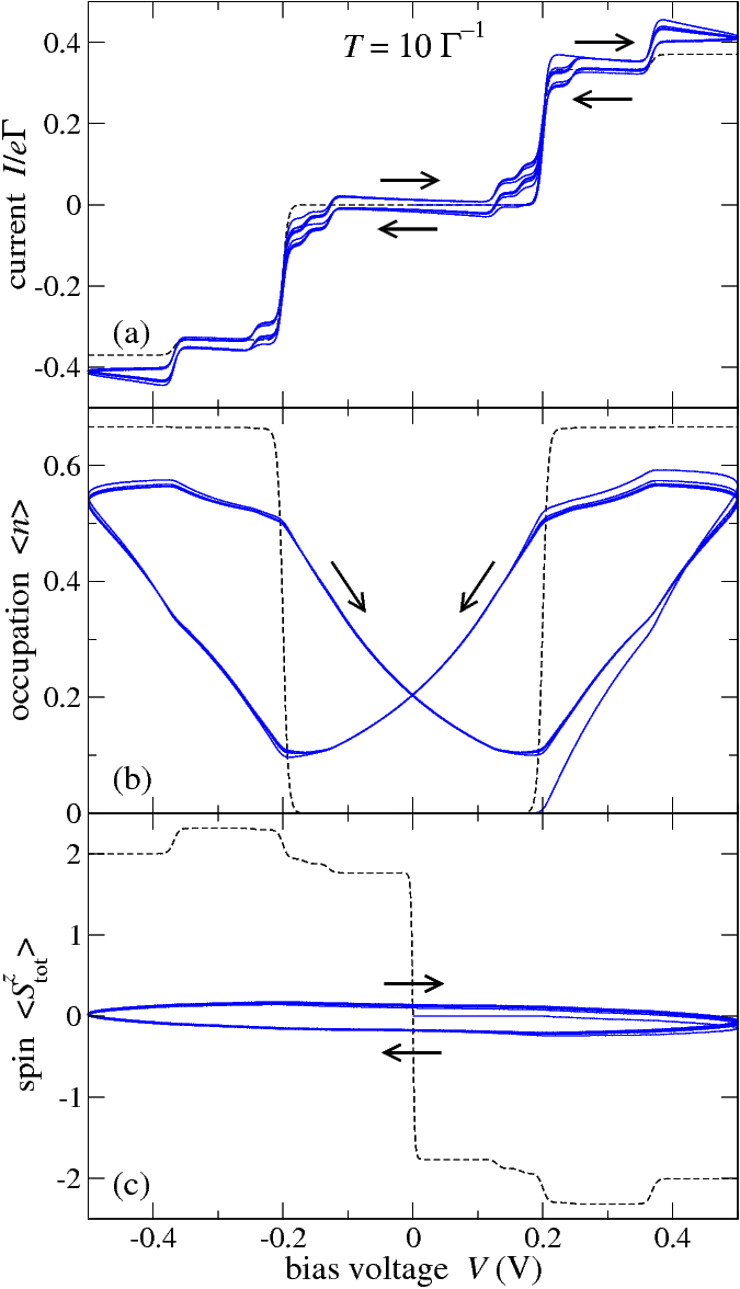
Figure 2: (Color online) (a) Current, (b) occupation number, and (c) z component of the total spin vs bias voltage for the SMM driven by a harmonic bias voltage of amplitude $V_{0}=0.5\,\mathrm{V}$ and period $T=10\,\Gamma^{-1}$. Ten full periods are shown as solid blue (gray) curves. The arrows indicate the directions in which the loops are traversed. The black dashed curves refer to the stationary state, corresponding to $T\to\infty$. The spin polarization in the leads is $p=N_{\mathrm{min}}/N_{\mathrm{maj}}=0.5$. The other model parameters are $\epsilon_{d}=0.2\,\mathrm{eV}$, $U=10\,\mathrm{eV}$, $J=0.1\,\mathrm{eV}$, $K_{2}=40\,\mathrm{meV}$, and $S=2$, as in Fig. 1.

Before analyzing the dependence on the period and the amplitude of the bias voltage in detail, let us show the typical behavior of our system for one parameter set. Figure 2 shows the approach to the periodic regime when the system is initialized in its equilibrium state at time $t=0$ and then driven by a bias $V(t)=V_{0}\,\sin\omega t$ with period $T=2\pi/\omega$. The current, occupation number, and the z component of the total spin approach periodic behavior within a few periods. As expected, all three observables show hysteresis. Since the state of the system evidently depends on its history, we immediately see that our system is indeed a memory device.PeV11 Its internal state is described by the probability vector $\mathbf{P}(t)$, which contains $N_{F}-1$ independent real variables, where $N_{F}$ is the dimension of the molecular Fock space. However, it is not a purely memristive system: A memristive system would satisfy equations of the formPeV11

$$I(t) = G\big{(}V(t),\mathbf{P}(t)\big{)}\,V(t),$$ (19)

$$\frac{d\mathbf{P}}{dt} = \mathbf{F}\big{(}V(t),\mathbf{P}(t)\big{)}.$$ (20)

In our case, the second equation is the master equation (6). On the other hand, our Eqs. (15) and (16) for the current cannot be written in the form of Eq. (19) for all $V$. Equation (19) implies that the current vanishes for zero bias for a memristive system, whereas Fig. 2 shows that it does not vanish for our device—the hysteresis loop is not pinched at $V=0$. Physically, this is because we have additional capacitive or inductive effects. The I-V characteristics of a harmonically driven pure capacitor (inductor) show an ellipse that is traversed in the clockwise (counterclockwise) direction. Since the loop in Fig. 2(a) is clockwise, the behavior is partially capacitive. This is reasonable since the molecule is transiently charged, as shown in Fig. 2(b).

For comparison, Fig. 2 also shows the voltage dependences of all observables in the stationary state (dashed curves). Note that the average spin in the stationary state is nonzero and depends on the bias voltage solely because the leads are magnetically polarized. If electrons are predominantly moving from left to right ($I<0$), the left lead injects predominantly spin-up electrons, while the right lead absorbs predominantly spin-down electrons. The result is a positive spin polarization on the molecule, as seen in Fig. 2(c). The stationary curves all show plateaus separated by thermally broadened steps. The dynamical current and charge mainly relax toward the stationary values at the plateaus but cannot follow the rapid changes at the steps. The visibility of the relaxation suggests that the driving period is comparable to the relevant relaxation times. On the other hand, the spin hysteresis loop bears no resemblance to the stationary curve, showing that the spin cannot relax rapidly enough to approach its stationary value. We will discuss these points in what follows.

IV.1 Dependence on the voltage period

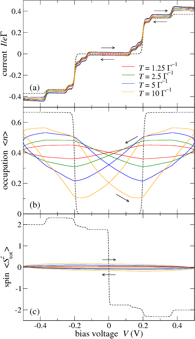
Figure 3: (Color online) (a) Current, (b) occupation number, and (c) z component of the total spin vs voltage for voltages of amplitude $V_{0}=0.5\,\mathrm{V}$ and relatively short periods $T=1.25$, $2.5$, $5$, and $10\,\Gamma^{-1}$. The other parameters are as in Fig. 2. A single hysteresis loop in the periodic regime is shown. The arrows indicate the directions in which the loops are traversed. The black dashed curves show the voltage dependence in the stationary state.

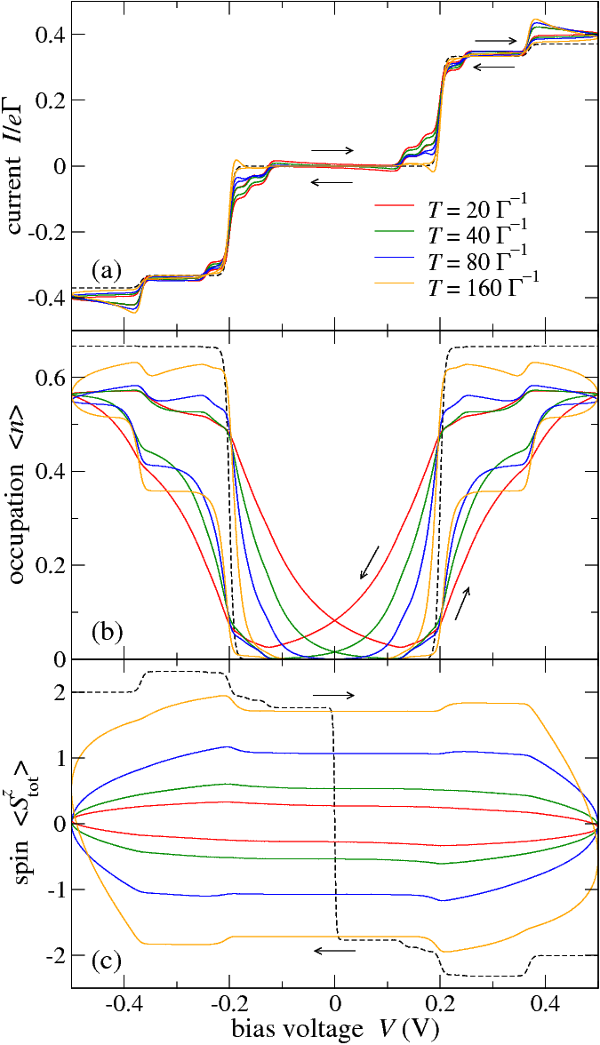
Figure 4: (Color online) (a) Current, (b) occupation number, and (c) z component of the total spin vs voltage for voltages of amplitude $V_{0}=0.5\,\mathrm{V}$ and intermediate periods $T=20$, $40$, $80$, and $160\,\Gamma^{-1}$. The other parameters are as in Fig. 2. A single hysteresis loop in the periodic regime is shown. The arrows indicate the directions in which the loops are traversed. Black dashed curves: Stationary state.

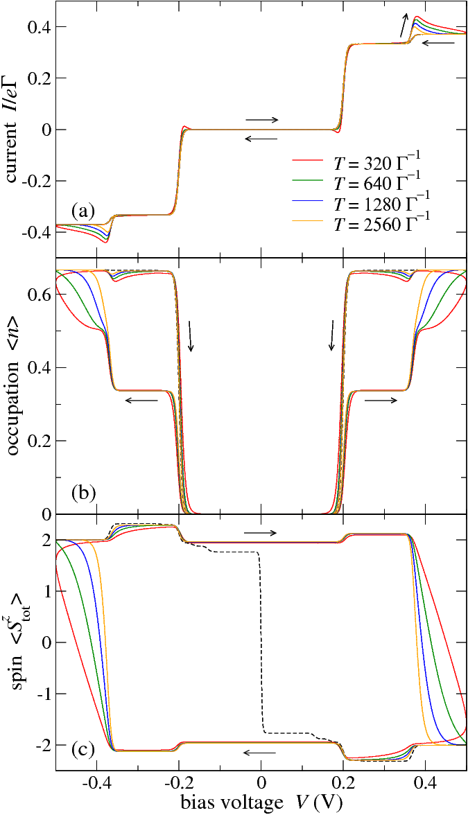
Figure 5: (Color online) (a) Current, (b) occupation number, and (c) z component of the total spin vs voltage for voltages of amplitude $V_{0}=0.5\,\mathrm{V}$ and relatively long periods $T=320$, $640$, $1280$, and $2560\,\Gamma^{-1}$. The other parameters are as in Fig. 2. A single hysteresis loop in the periodic regime is shown. The arrows indicate the directions in which the loops are traversed. Black dashed curves: Stationary state.

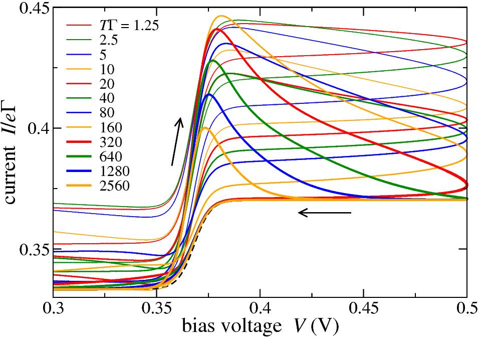
Figure 6: (Color online) Details of the current vs voltage curves for periods $T=1.25$, …, $2560\,\Gamma^{-1}$ from Figs. 3, 4, and 5. The arrows indicate the direction in which the hysteresis loops are traversed. Black dashed curve: Stationary state.

To elucidate the role of the driving period $T$, we have determined the periodic behavior for various $T$’s as described in Sec. III, keeping all other parameters fixed. Figures 3, 4, and 5 show single hysteresis loops for current, charge, and spin in the periodic regime. Since the hysteresis in the current is not very pronounced on the scale of the figures, we show an enlargement close to the voltage maximum in Fig. 6. The natural time scale is $\Gamma^{-1}=(2\pi|t_{\mathrm{hyb}}|^{2}N_{\mathrm{maj}})^{-1}$, the inverse of the characteristic tunneling rate. Note that for a typical current of $200\,\mathrm{pA}$ in the transmitting regime,PPL00 ; HGF06 the tunneling rate is on the order of $\Gamma\approx 10^{9}\,\mathrm{s}^{-1}$. In the limit of rapid driving ($T\to 0$), shown in Fig. 3, all hysteresis loops close since the molecule cannot follow the rapid bias. The charge and the spin approach constant values determined by the time-averaged rates,

$$\overline{R}_{n\to m}=\frac{1}{T}\int_{0}^{T}dt\,R_{n\to m}(t).$$ (21)

The current loop also closes but it does not become a horizontal line since the current in Eq. (15) explicitly depends on the instantaneous rates, which in turn depend on the instantaneous bias.

We note that the hysteresis loops for the current, in particular at rapid driving, show additional steplike features absent from the stationary curves. These features are due to excited-state-to-excited-state (ETE) transitions. Such transitions are also observed in the stationary state,GTT08 but only if the energy of the ETE transition is higher than the energy of the transition populating its initial state. This restriction is relaxed for dynamical measurements, where the initial state can be transiently occupied even when the voltage is not sufficiently high to populate it in the stationary regime. Thus, additional spectroscopic information on ETE transition energies and lifetimes (from the width of the current steps) can be obtained from dynamical measurements.

In the limit of slow driving, $T\to\infty$, the hysteresis loops must also close since the observables approach the stationary values. The current loops in Fig. 5(a) indeed close for slow driving. In particular, the capacitive response (open loop at $V=0$) decreases rapidly together with the charge at zero voltage. However, the charge and the spin in Figs. 5(b) and 5(c), respectively, have not approached the stationary curve even at $T=2560\,\Gamma^{-1}$. The reason for this requires some discussion.

All quantities show steplike behavior for large $T$ with two pairs of steps at voltages of about $\pm 0.20\,\mathrm{V}$ and about $\pm 0.37\,\mathrm{V}$. It is useful to refer to the level scheme in Fig. 1 to understand what happens at these voltages. At $|V|=V_{1}\equiv 2(E_{1,\pm 5/2}-E_{0,\pm 2})=0.2\,\mathrm{V}$, the excess energy $eV/2$ of electrons appearing in Eqs. (8)–(11) matches the lowest transition energy $E_{1,\pm 5/2}-E_{0,\pm 2}$ out of the ground states with occupation number $n=0$ and magnetic quantum numbers $m=\pm 2$ to the states $n=1$, $m=\pm 5/2$. These transitions are denoted by solid arrows in Fig. 1. From the excited states $n=1$, $m=\pm 5/2$, the molecule can only relax back to the ground states by emitting one electron into the leads. No other transitions are allowed for sequential tunneling. Thus the molecule cannot overcome the anisotropy barrier and the imbalance $\Delta M\equiv\langle\mathrm{sgn}(S_{\mathrm{tot}}^{z})\rangle$ between positive and negative $m$ cannot be relaxed.TiE06 In fact, this statement is only rigorously true at zero temperature. At finite temperatures, there is a thermally activated process in which the molecule goes from the ground states to a state with $n=1$, $m=\pm 3/2$ (dashed arrows in Fig. 1), but the transition rate for this process is exponentially suppressed by the tail of the Fermi function.

At the second step at $|V|=V_{2}\equiv 2(E_{1,\pm 3/2}-E_{0,\pm 2})=0.367763\,\mathrm{V}$, the excess energy $eV/2$ matches the transition energy $E_{1,\pm 3/2}-E_{0,\pm 2}$ from the ground states to a state with $n=1$ and $m=\pm 1/2$ (dashed arrows in Fig. 1). But then the molecule can overcome the anisotropy barrier by a series of sequential-tunneling transitions that are either exothermal or endothermal with a transition energy lower than $eV_{2}/2$. Consequently, for voltages close to $V_{2}$, the rate for spin relaxation over the barrier crosses over from exponentially small to a sizable fraction of $\Gamma$.TiE06 Relaxation over the barrier is still slower than relaxation not crossing the barrier since it involves several sequential-tunneling transitions, each of which competes with a transition in the opposite direction.

We can now understand the behavior of the spin for slow driving in Fig. 5: Above the second threshold, $V>V_{2}$, relaxation over the barrier is not exponentially suppressed, and the system indeed approaches the stationary behavior for slow driving. As the voltage is lowered into the range $V_{1}<V<V_{2}$, the imbalance $\Delta M$ between positive and negative $m$ is frozen in. As long as the driving is not exponentially slow, the system will relax under the constraint of fixed $\Delta M$. In the range $V_{1}<V<V_{2}$ the frozen-in value of $\Delta M$ is close to the stationary value so that the system can still relax to a state close to the stationary one. When the voltage falls below $V_{1}$, all transitions out of the two ground states in Fig. 1 are thermally suppressed, and the system relaxes toward the ground states with the imbalance $\Delta M$ approximately conserved.

For $-V_{2}<V<-V_{1}$, the lowest-energy transitions become active again but now the frozen value of $\Delta M$ is very different from the stationary one at negative voltages. The system is still with a high probability on the left-hand side of the barrier ($\Delta M<0$). The most relevant transition is the one from the state $n=0$, $m=-2$ to the state $n=1$, $m=-5/2$, which requires a spin-down electron. However, for negative voltages predominantly spin-up electrons are injected. The transition rate for this process is thus suppressed by the spin-polarization factor $p$ in Eq. (9). Consequently, the average occupation $\langle n\rangle$ is suppressed relative to the stationary case, leading to the plateau at $\langle n\rangle\approx 0.336$ in Fig. 5(b). Finally, for $V<-V_{2}$, spin relaxation over the barrier becomes active again, the imbalance $\Delta M$ is unfrozen, and the system can relax to the stationary state at slow driving.

In summary, the device does approach the stationary regime in the limit of slow driving, $T\to\infty$, but to reach this regime, the period $T$ has to be large compared to the exponentially long spin relaxation time. We thus find a separation of time scales: The spin relaxation time is generically long compared to typical relaxation times for processes not crossing the anisotropy barrier. This can be compared to the dynamics of a molecule without local spin but involving a vibrational mode:DYG12 ; Koch In this case small Franck-Condon matrix elements suppressing low-energy transitions can lead to a separation of time scales.

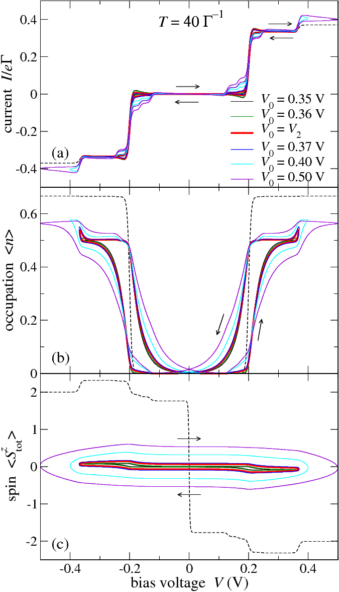
Figure 7: (Color online) (a) Current, (b) occupation number, and (c) z component of the total spin vs voltage for voltage amplitudes $V_{0}=0.35\,\mathrm{V}$, $0.36\,\mathrm{V}$, $0.367763\,\mathrm{V}$ (${=}\>V_{2}$), $0.37\,\mathrm{V}$, $0.40\,\mathrm{V}$, and $0.50\,\mathrm{V}$ and period $T=40\,\Gamma^{-1}$. The other parameters are as in Figs. 2–5. A single hysteresis loop in the periodic regime is shown in each case; the loop at the threshold amplitude, $V_{0}=V_{2}$, is highlighted as a heavy red (gray) curve. The arrows indicate the directions in which the loops are traversed. The black dashed curves show the voltage dependence in the stationary state.

IV.2 Dependence on the voltage amplitude

Since the imbalance $\Delta M$ between positive and negative magnetic quantum numbers is effectively frozen in when the voltage drops below the threshold $V_{2}$, we expect the behavior of the device to change dramatically when the amplitude $V_{0}$ of the bias $V(t)=V_{0}\,\sin\omega t$ is tuned through $V_{2}$. To exhibit this dependence, we have determined the periodic behavior for amplitudes $V_{0}$ through the threshold $V_{2}$, keeping all other parameters fixed. Figure 7 shows single hysteresis loops for current, charge, and spin in the periodic regime. As expected, the spin hysteresis loops are nearly closed for voltage amplitudes $V_{0}$ below the threshold $V_{2}$ and open up above the threshold. Then the system can overcome the barrier for part of the driving period so that the spins injected from the magnetized leads can reverse the local spin.

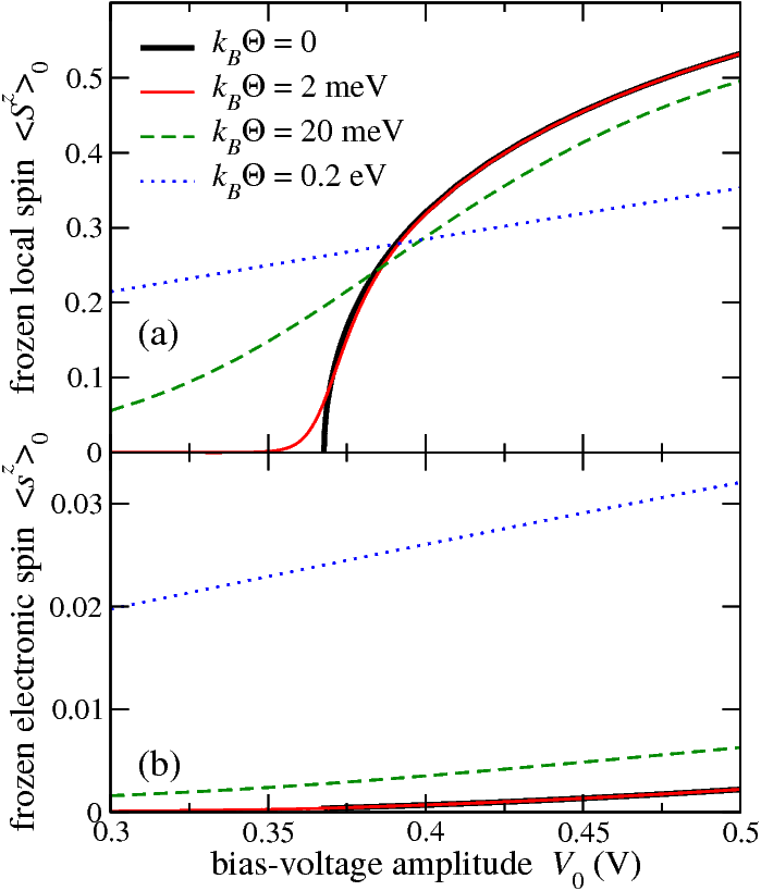
Figure 8: (Color online) (a) Frozen local spin $\langle S^{z}\rangle_{0}$ and (b) frozen electronic spin $\langle s^{z}\rangle_{0}$ at $V(t)=0$ and $V^{\prime}(t)>0$ vs voltage amplitude at thermal energies $k_{B}\Theta=0$, $2\,\mathrm{meV}$, $20\,\mathrm{meV}$, and $0.2\,\mathrm{eV}$. The other parameters are as in Fig. 7.

A reasonable measure of the size of the spin hysteresis loop—which represents the effectiveness of the device in storing information—is the frozen spin at $V=0$ with $V^{\prime}(t)>0$. We plot the local and the electronic contributions to the frozen spin as functions of the voltage amplitude for zero and finite temperatures in Fig. 8. To obtain the values at zero temperature, we proceed differently from the method outlined in Sec. III: For $k_{B}\Theta=0$, the Fermi function becomes a step function and thus the transition rates in Eqs. (8)–(11) are piecewise constant functions of the instantaneous voltage $V(t)$ and, therefore, of time. This allows us to obtain the stochastic matrix $\Pi$ analytically as a product of a finite number of matrices describing the time evolution over time intervals with constant rates.

The frozen local spin $\langle S^{z}\rangle_{0}$ in Fig. 8(a) shows critical behavior for vanishing temperature. Taking the square we find that the critical exponent is $1/2$, $\langle S^{z}\rangle_{0}\sim(V_{0}-V_{2})^{1/2}$. The singularity is smeared out at finite temperatures. For the frozen electronic spin, critical behavior is not evident.

The origin of the exponent $1/2$ is that the fraction of time during which the voltage is large enough to overcome the barrier scales with $(V_{0}-V_{2})^{1/2}$ provided that $V(t)$ is analytic close to its extrema. Taking, for example, the first voltage maximum, the end points of this time interval are obtained by solving $V(T/4\pm\Delta t/2)=V_{2}$. If $V(t)$ is analytic, we can expand around the maximum, $V_{0}+V^{\prime\prime}(T/4)\Delta t^{2}/8=V_{2}$, the solution of which gives $\Delta t\sim(V_{0}-V_{2})^{1/2}$. We now expand the stochastic matrix $\Pi$ for small $\Delta t$ and use perturbation theory to find the probability vector for the periodic state satisfying $\mathbf{P}^{\mathrm{per}}=\Pi\,\mathbf{P}^{\mathrm{per}}$. The leading correction is linear in $\Delta t$ and thus proportional to $(V_{0}-V_{2})^{1/2}$.

We can therefore draw two conclusions: (i) Quite generally, all observables should inherit a $(V_{0}-V_{2})^{1/2}$ correction from $\mathbf{P}^{\mathrm{per}}$ above the threshold. (ii) The same argument also applies whenever additional transitions become energetically allowed at higher voltage amplitudes. Thus there should be corresponding singular terms associated with these transitions. We have checked that this is borne out by the numerical results.

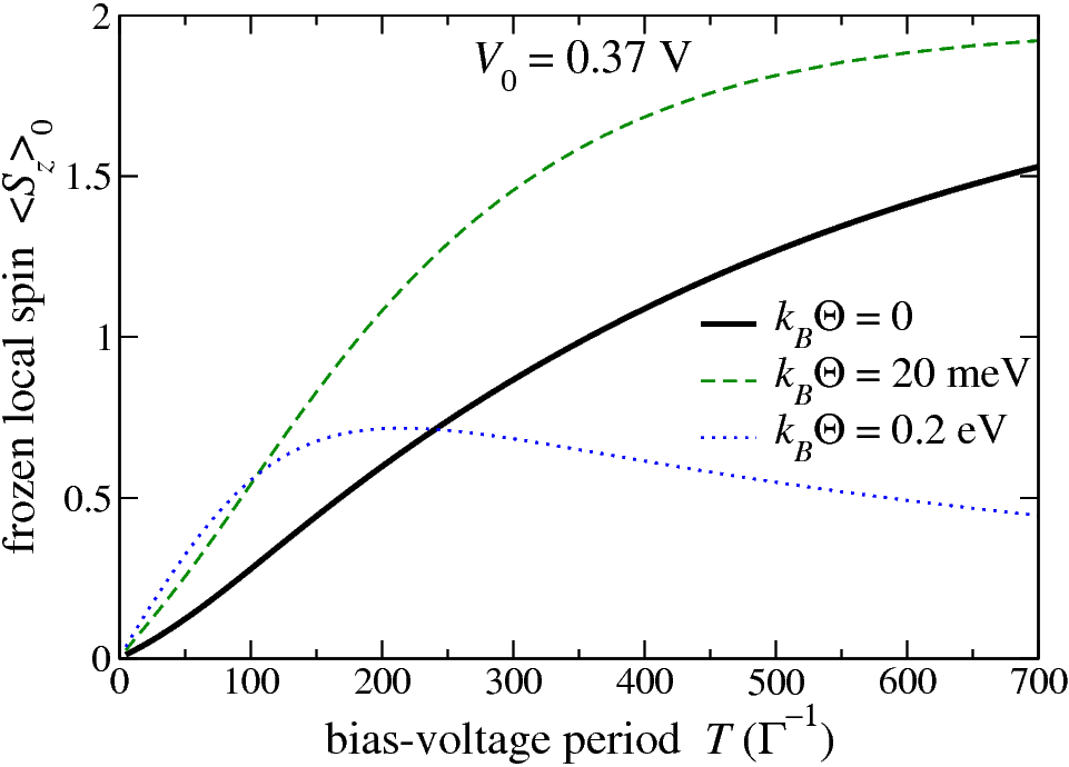
Figure 9: (Color online) Frozen local spin $\langle S^{z}\rangle_{0}$ vs voltage period at thermal energies $k_{B}\Theta=0$, $20\,\mathrm{meV}$, and $0.2\,\mathrm{eV}$. The voltage amplitude is $V_{0}=0.37\,\mathrm{V}$, slightly above the threshold $V_{2}$. The other parameters are as in Fig. 7.

We now turn to the dependence of the frozen spin on the driving frequency. Figure 9 shows the frozen local spin $\langle S^{z}\rangle_{0}$ as a function of the voltage period $T$ for three temperature values. The voltage amplitude $V_{0}$ is slightly above the threshold $V_{2}$ for spin relaxation. At rapid driving, $T\to 0$, the frozen spin goes to zero, as expected since the system cannot follow the rapidly changing bias. For very large periods, the frozen spin should approach the stationary value at zero bias, which is also zero. For the (unphysically) high temperature $k_{B}\Theta=0.2\,\mathrm{eV}$, Fig. 9 indeed shows this behavior. On the other hand, at zero temperature, the frozen spin never approaches zero for large $T$ since there is no spin relaxation for $|V(t)|<V_{2}$ so that the system can never reach the stationary state with zero average spin at zero bias.

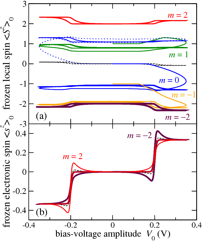
Figure 10: (Color online) (a) Solid curves: Five periods of the z component of the total spin, $\langle S^{z}_{\mathrm{tot}}\rangle$, vs voltage for different initial pure states with occupation number $n=0$ and magnetic quantum numbers $m=2$, $1$, $0$, $-1$, and $-2$. The voltage amplitude is $V_{0}=0.35\,\mathrm{V}<V_{2}$ and the voltage period is $T=40\,\Gamma^{-1}$. The other parameters are as in Figs. 2–5. Dotted curve: The same for the initial state with $m=0$ but for the voltage shifted in time by half a period. (b) Solid curves: Five periods of the current for the two cases with $m=2$ and $m=-2$. The parameters are the same as in (a). The black dashed curves show the true periodic state that the system would reach after an exponentially long time.

IV.3 Quasiperiodic regime

As we have seen, the anisotropy barrier leads to a separation of time scales for relaxation over the barrier and relaxation staying on one side of the barrier. It thus makes sense to consider the intermediate regime reached after the fast transients have died out, but before the slow relaxation has become effective. We call this the “quasiperiodic” regime.

As discussed above, the true periodic state is unique since it is determined by the stationary solution of an ergodic discrete-time Markov process. Thus the system will eventually converge to the same periodic solution regardless of its initial state. However, the same is not true for the quasiperiodic state, which will depend on the initial condition and, in principle, also on the protocol with which the bias is switched on. This is illustrated in Fig. 10(a), which shows the first five periods of the time evolution of the total spin $\langle S^{z}_{\mathrm{tot}}\rangle$ starting from different initial states. The voltage amplitude is $V_{0}=0.35\,\mathrm{V}<V_{2}$ so that the relaxation over the barrier is exponentially slow. After a few periods, a quasiperiodic regime is reached, which indeed depends on the initial state. After a much longer time, during which the system can relax over the barrier, all curves would approach the true periodic hysteresis loop (dashed curve).

We have also verified that the quasiperiodic loop does depend on the way the voltage is switched on. The dotted blue (gray) curve in Fig. 10(a) shows the spin for the same initial state as the solid blue (gray) curve; the only difference is that the voltage is shifted in time by half a period, i.e., $V(t)=-V_{0}\sin\omega t$. Since the system starts in the state with $m=0$, which is the one on top of the anisotropy barrier in Fig. 1, the sign of the voltage applied during the first half period determines the dominant spin direction of the injected electrons. This determines the probabilities for the system to relax into states with positive or negative $m$. The resulting imbalance $\Delta M$ is then frozen in because the voltage amplitude is below the threshold $V_{2}$. Consequently, the sign of $V(t)$ during the first half period determines the spin polarization.

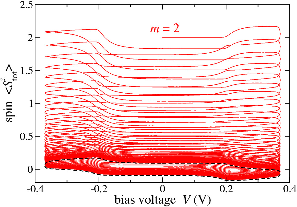
Figure 11: (Color online) Solid red (gray) curve: $50$ periods of the z component of the total spin vs voltage for the initial pure state with occupation number $n=0$ and magnetic quantum number $m=2$. The voltage amplitude is $V_{0}=0.37\,\mathrm{V}>V_{2}$ and the voltage period is $T=40\,\Gamma^{-1}$. The other parameters are as in Fig. 10. Dashed black curve: Periodic state.

It is illuminating to compare the behavior when the voltage amplitude is above the threshold $V_{2}$. In this case, we do not expect a separation of time scales. Figure 11 indeed shows that the spin approaches the periodic hysteresis loop without reaching any intermediate quasiperiodic regime. The relaxation over the barrier is still slow since it involves several sequential-tunneling transitions and is only active for a small fraction of the time.

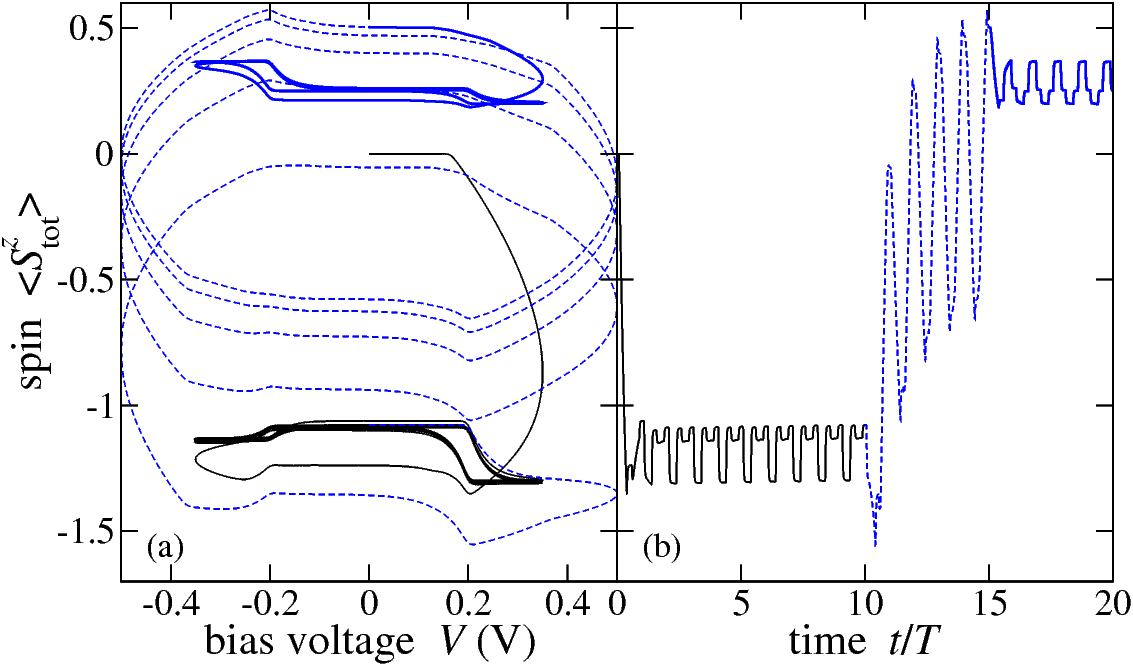
Figure 12: (Color online) z component of the total spin vs (a) voltage and (b) time, for a process starting from the pure state with $n=0$ and $m=0$ and consisting of ten periods at the amplitude $V_{0}=0.35\,\mathrm{V}<V_{2}$, five periods at $V_{0}=0.5\,\mathrm{V}>V_{2}$, and five periods at $V_{0}=0.35\,\mathrm{V}<V_{2}$. The voltage period is held fixed to $T=40\,\Gamma^{-1}$. The other parameters are as in the previous figures.

The spin polarization in the intermediate, quasiperiodic regime can be read out by a transport experiment: Figure 10(b) shows the current hysteresis loops for the two cases with initial value $m=\pm 2$ (solid curves) and also the true periodic behavior (dashed curve). The loops are clearly different. To use our model system as a memory device, we also need a protocol for writing the spin. This is possible by increasing the voltage amplitude over the threshold, and making the period $T$ sufficiently long. Then the spin approaches a large hysteresis loop on a time scale of a few periods. Reducing the voltage amplitude below the threshold while the spin is large in magnitude freezes the imbalance $\Delta M$. For illustration, we plot in Fig. 12 the spin for a process starting from the pure state with $n=0$ and $m=0$ and consisting of ten periods at a small voltage amplitude $V_{0}<V_{2}$, followed by five periods at $V_{0}>V_{2}$, and eventually by five more periods at the smaller amplitude. Figure 12 shows the spin as a function of bias and of time. This protocol clearly switches the system between two distinct quasiperiodic states. If we had reduced the amplitude half of a period earlier or later, i.e., when $\langle S^{z}_{\mathrm{tot}}\rangle$ was negative, a negative spin would have been written.

The typical time scale of the switching in Fig. 12 is a few times $T=40\,\Gamma^{-1}\sim 4\times 10^{-8}\,\mathrm{s}$. This should be compared to the switching time of memristive systems containing a MgO layer between ferromagnetic electrodes, which is on the order of seconds, probably because it involves the displacement of oxygen vacancies.HMB08 ; KKR09 The switching mechanism proposed in the present paper can be much faster since it involves neither nuclear motion, as Refs. HMB08, and KKR09, and also the spin transition considered by Miyamachi et al.MGD12 do, nor the motion of domain walls, which is the mechanism studied by Münchenberger et al.MRT12

V Summary and conclusions

Memristive (memory resistive) properties of a SMM weakly coupled to two ferromagnetic leads have been investigated. To that end, we have studied three observables: the average current through the molecule, the occupation (charge), and the z component of the total spin on the molecule. We have obtained the hysteresis loops for these quantities vs the applied bias. The device is not a purely memristive system, as evidenced by the open hysteresis loop for the current. Instead, the transient charging of the molecule leads to a partially capacitive response. This capacitive response is governed by the fast charge relaxation. The device combines memristive with spintronics functionality facilitated by a large polarization of the molecular spin.

For rapid driving, i.e., for driving frequencies on the order of the characteristic tunneling rate $\Gamma$, the memory dependence is suppressed and the hysteresis loops close. The current-voltage characteristics nevertheless show additional spectroscopic features not seen in the stationary (dc) current-voltage curve. In the opposite limit of very slow driving, memory effects are also suppressed since the system eventually approaches the stationary behavior. However, the period of the voltage required to reach this stationary regime can be exceedingly long in the presence of easy-axis anisotropy. The origin of this dynamical slowing down is that relaxation of the molecular spin over the anisotropy barrier becomes suppressed below a certain bias voltage so that any imbalance between positive and negative spin polarization is essentially frozen in. It is the very slow relaxation over the barrier that governs the eventual closing of the hysteresis loops.

At zero temperature, the frozen occupation number and spin at zero bias exhibit non-analyticities when the voltage amplitude crosses the threshold for relaxation over the barrier. The non-analytic contributions scale with the voltage distance from the transition point with a critical exponent of $1/2$. The singular behavior is smeared out at finite temperatures.

We have seen that the easy-axis anisotropy naturally leads to a separation of time scales: If the bias voltage is below a critical threshold, relaxation over the barrier is exponentially suppressed compared to relaxation between states on the same side of the barrier, by the tail of the Fermi function appearing in the sequential-tunneling rates. Now, the question arises as to whether any processes neglected in our approach become relevant in this regime. Sequential tunneling is of the order of $t_{\mathrm{hyb}}^{2}\propto\Gamma$. At the order $t_{\mathrm{hyb}}^{4}\propto\Gamma^{2}$, cotunneling occurs: An electron can tunnel coherently from one lead to the other. During this process, it can flip its spin, which leads to a transition of the molecular state without a change of the occupation number, but with a change of the spin by one unit. Out of the ground states, this process becomes active when $eV$ matches the energy difference $eV_{\mathrm{cot}}\equiv E_{0,\pm 1}-E_{0,\pm 2}$ between the states with $m=\pm 1$ and $m=\pm 2$, which for the parameters chosen here happens at a voltage below the Coulomb-blockade threshold $V_{1}$, see Fig. 1. (Note that the full bias $eV$ enters in this case.) Beyond the voltage $V_{\mathrm{cot}}$, the system can overcome the anisotropy barrier by cotunneling. Thus there is a regime where relaxation over the barrier is dominated by cotunneling, which is down by a factor of $\Gamma$ compared to sequential tunneling, but does not involve an exponentially small factor at low temperatures. At smaller voltages, $|V|<V_{\mathrm{cot}}$, cotunneling is also exponentially suppressed and processes of even higher order in $\Gamma$ become important. Eventually, the direct transition from one ground state to the other involving a change of the spin by four units occurs at order $\Gamma^{8}$. This process happens even at zero bias and is thus never suppressed by exponential factors.

Still, below the threshold $V_{2}$ for spin relaxation due to sequential tunneling, the relaxation rate is at least suppressed by a factor of $\Gamma$. Thus, for sufficiently weak coupling between the molecule and the leads, there is still a wide separation of time scales. We finally note that transverse spin-anisotropy terms, or a transverse magnetic field, can lead to spin tunneling through the barrier and thereby open another channel for spin relaxation.

The separation of time scales opens up an intermediate time regime where fast transients have died out, but relaxation over the barrier has yet to become effective. In this regime, a quasiperiodic dependence of all observables on the bias is observed. Unlike the true periodic state, the quasiperiodic hysteresis loop depends on the initial conditions and the protocol by which the bias is switched on. In view of the long lifetime that can be realized experimentally, this means that this property can be used to store information. Indeed, we have demonstrated that this spin information can be read out by measuring the alternating current, and that it can be rewritten at will by judiciously changing the voltage amplitude. Note that we have discussed a two-terminal device. None of this functionality requires a gate electrode (although the latter would add extra flexibility), which should make the practical implementation significantly easier.

Finally, it is also worth noting that the presence of different time scales and long relaxation times makes molecular magnets ideally suited for a host of neuromorphic applications,pershin12a ranging from learning circuitspershin09b and associative memorypershin10c to the massively parallel solution of optimization problems.pershin11d While neuromorphic and memristive devices based on magnetic solid-state structures have been suggested,HMB08 ; KKR09 ; MRT12 ; SAP12 molecular magnets potentially offer higher integration densities, faster switching, and lower power consumption. These features make them ideal candidates for neuromorphic computing.

- (1) J. Park, A. N. Pasupathy, J. I. Goldsmith, C. Chang, Y. Yaish, J. R. Petta, M. Rinkoski, J. P. Sethna, H. D. Abruña, P. L. McEuen, and D. C. Ralph, Nature (London) 417, 722 (2002).
- (2) W. Liang, M. P. Shores, M. Bockrath, J. R. Long, and H. Park, Nature (London) 417, 725 (2002).
- (3) H. B. Heersche, Z. de Groot, J. A. Folk, H. S. J. van der Zant, C. Romeike, M. R. Wegewijs, L. Zobbi, D. Barreca, E. Tondello, and A. Cornia, Phys. Rev. Lett. 96, 206801 (2006).
- (4) M.-H. Jo, J. E. Grose, K. Baheti, M. M. Deshmukh, J. J. Sokol, E. M. Rumberger, D. N. Hendrickson, J. R. Long, H. Park, and D. C. Ralph, Nano Lett. 6, 2014 (2006).
- (5) J. J. Henderson, C. M. Ramsey, E. del Barco, A. Mishra, and G. Christou, J. Appl. Phys. 101, 09E102 (2007).
- (6) J. E. Grose, E. Tam, C. Timm, M. Scheloske, B. Ulgut, J. J. Parks, H. D. Abruña, W. Harneit, and D. C. Ralph, Nature Mater. 7, 884 (2008).
- (7) C. Iacovita, M. V. Rastei, B. W. Heinrich, T. Brumme, J. Kortus, L. Limot, and J.-P. Bucher, Phys. Rev. Lett. 101, 116602 (2008).
- (8) G. D. Scott, Z. K. Keane, J. W. Ciszek, J. M. Tour, and D. Natelson, Phys. Rev. B 79, 165413 (2009).
- (9) A. S. Zyazin, J. W. G. van den Berg, E. A. Osorio, H. S. J. van der Zant, N. P. Konstantinidis, M. Leijnse, M. R. Wegewijs, F. May, W. Hofstetter, C. Danieli, and A. Cornia, Nano Lett. 10, 3307 (2010).
- (10) N. Roch, R. Vincent, F. Elste, W. Harneit, W. Wernsdorfer, C. Timm, and F. Balestro, Phys. Rev. B 83, 081407(R) (2011).
- (11) T. Komeda, H. Isshiki, J. Liu, Y.-F. Zhang, N. Lorente, K. Katoh, B. K. Breedlove, and M. Yamashita, Nature Commun. 2, 217 (2011).
- (12) A. Mugarza, C. Krull, R. Robles, S. Stepanow, G. Ceballos, and P. Gambardella, Nature Commun. 2, 490 (2011).
- (13) T. Miyamachi, M. Gruber, V. Davesne, M. Bowen, S. Boukari, L. Joly, F. Scheurer, G. Rogez, T. K. Yamada, P. Ohresser, E. Beaurepaire, and W. Wulfhekel, Nature Commun. 3, 938 (2012).
- (14) F. Elste and C. Timm, Phys. Rev. B 71, 155403 (2005).
- (15) C. Romeike, M. R. Wegewijs, and H. Schoeller, Phys. Rev. Lett. 96, 196805 (2006).
- (16) M. N. Leuenberger and E. R. Mucciolo, Phys. Rev. Lett. 97, 126601 (2006); G. González, M. N. Leuenberger, and E. R. Mucciolo, Phys. Rev. B 78, 054445 (2008).
- (17) C. Timm and F. Elste, Phys. Rev. B 73, 235304 (2006).
- (18) F. Elste and C. Timm, Phys. Rev. B 73, 235305 (2006).
- (19) J. Lehmann and D. Loss, Phys. Rev. Lett. 98, 117203 (2007).
- (20) M. Misiorny and J. Barnaś, EPL 78, 27003 (2007); Phys. Rev. B 76, 054448 (2007); ibid. 77, 172414 (2008).
- (21) G. González and M. N. Leuenberger, Phys. Rev. Lett. 98, 256804 (2007).
- (22) P. S. Cornaglia, G. Usaj, and C. A. Balseiro, Phys. Rev. B 76, 241403(R) (2007).
- (23) T. Jonckheere, K.-I. Imura, and T. Martin, Phys. Rev. B 78, 045316 (2008).
- (24) F. Reckermann, M. Leijnse, and M. R. Wegewijs, Phys. Rev. B 79, 075313 (2009).
- (25) H.-Z. Lu, B. Zhou, and S.-Q. Shen, Phys. Rev. B 79, 174419 (2009).
- (26) M. Misiorny, I. Weymann, and J. Barnaś, Phys. Rev. B 79, 224420 (2009); EPL 89, 18003 (2010).
- (27) F. Elste and C. Timm, Phys. Rev. B 81, 024421 (2010).
- (28) A. Soncini and L. F. Chibotaru, Phys. Rev. B 81, 132403 (2010).
- (29) R. Jaafar, E. M. Chudnovsky, and D. A. Garanin, EPL 89, 27001 (2010).
- (30) Z. G. Yu, J. Phys.: Condens. Matter 22, 295305 (2010).
- (31) P. S. Cornaglia, P. Roura Bas, A. A. Aligia, and C. A. Balseiro, EPL 93, 47005 (2011).
- (32) M. Misiorny, I. Weymann, and J. Barnaś, Phys. Rev. Lett. 106, 126602 (2011); Phys. Rev. B 84, 035445 (2011).
- (33) C. López-Monís, C. Emary, G. Kiesslich, G. Platero, and T. Brandes, Phys. Rev. B 85, 045301 (2012).
- (34) N. Bode, L. Arrachea, G. S. Lozano, T. S. Nunner, and F. von Oppen, Phys. Rev. B 85, 115440 (2012).
- (35) R. Sessoli, D. Gatteschi, A. Caneschi, and M. A. Novak, Nature (London) 365, 141 (1993).
- (36) J. R. Friedman and M. P. Sarachik, Annu. Rev. Condens. Matter Phys. 1, 109 (2010).
- (37) Y. V. Pershin and M. Di Ventra, Phys. Rev. B 78, 113309 (2008).
- (38) L. O. Chua and S. M. Kang, Proc. IEEE 64, 209 (1976).
- (39) M. Di Ventra, Y. V. Pershin, and L. O. Chua, Proc. IEEE 97, 1717 (2009).
- (40) Y. V. Pershin and M. Di Ventra, Adv. Phys. 60, 145 (2011).
- (41) Y. V. Pershin, S. La Fontaine, and M. Di Ventra, Phys. Rev. E 80, 021926 (2009).
- (42) Y. V. Pershin and M. Di Ventra, Neural Networks 23, 881 (2010).
- (43) Y. V. Pershin and M. Di Ventra, Proc. IEEE 100, 2071 (2012).
- (44) X. Wang, Y. Chen, H. Xi, H. Li, and D. Dimitrov, IEEE El. Device Lett. 30, 294 (2009).
- (45) A. Donarini, A. Yar, and M. Grifoni, arXiv:1205.4927.
- (46) J. Koch and F. von Oppen, Phys. Rev. Lett. 94, 206804 (2005); J. Koch, M. E. Raikh, and F. von Oppen, ibid. 95, 056801 (2005).
- (47) S. Nakajima, Prog. Theor. Phys. 20, 948 (1958).
- (48) R. Zwanzig, J. Chem. Phys. 33, 1338 (1960); Physica 30, 1109 (1964).
- (49) M. Tokuyama and H. Mori, Prog. Theor. Phys. 55, 411 (1976).
- (50) N. Hashitsume, F. Shibata, and M. Shingū, J. Stat. Phys. 17, 155 (1977); F. Shibata, Y. Takahashi, and N. Hashitsume, ibid. 17, 171 (1977).
- (51) D. Ahn, Phys. Rev. B 50, 8310 (1994).
- (52) H.-P. Breuer and F. Petruccione, The Theory of Open Quantum Systems (Oxford University Press, Oxford, 2002).
- (53) C. Timm, Phys. Rev. B 83, 115416 (2011).
- (54) A. Mitra, I. Aleiner, and A. J. Millis, Phys. Rev. B 69, 245302 (2004).
- (55) C. Timm, Phys. Rev. B 77, 195416 (2008).
- (56) M. Di Ventra, Electrical Transport in Nanoscale Systems (Cambridge University Press, Cambridge, 2008).
- (57) M. P. Anantram and S. Datta, Phys. Rev. B 51, 7632 (1995).
- (58) B. Wang, J. Wang, and H. Guo, Phys. Rev. Lett. 82, 398 (1999).
- (59) Y. Xing, B. Wang, and J. Wang, Phys. Rev. B 82, 205112 (2010).
- (60) Computer code mathematica, version 8.0 (Wolfram Research, Champaign, IL, 2010).
- (61) H. Park, J. Park, A. K. L. Lim, E. H. Anderson, A. P. Alivisatos, and P. L. McEuen, Nature (London) 407, 57 (2000).
- (62) D. Halley, H. Majjad, M. Bowen, N. Najjari, Y. Henry, C. Ulhaq-Bouillet, W. Weber, G. Bertoni, J. Verbeeck, and G. Van Tendeloo, Appl. Phys. Lett. 92, 212115 (2008).
- (63) P. Krzysteczko, X. Kou, K. Rott, A. Thomas, and G. Reiss, J. Magn. Magn. Mat. 321, 144 (2009); P. Krzysteczko, G. Reiss, and A. Thomas, Appl. Phys. Lett. 95, 112508 (2009).
- (64) J. Münchenberger, G. Reiss, and A. Thomas, J. Appl. Phys. 111, 07D303 (2012).
- (65) Y. V. Pershin and M. Di Ventra, Phys. Rev. E 84, 046703 (2011).
- (66) M. Sharad, C. Augustine, G. Panagopoulos, and K. Roy, arXiv:1206.2466; arXiv:1206.3227.