Nonlinear shrinkage estimation of large-dimensional covariance matrices

Abstract

Many statistical applications require an estimate of a covariance matrix and/or its inverse. When the matrix dimension is large compared to the sample size, which happens frequently, the sample covariance matrix is known to perform poorly and may suffer from ill-conditioning. There already exists an extensive literature concerning improved estimators in such situations. In the absence of further knowledge about the structure of the true covariance matrix, the most successful approach so far, arguably, has been shrinkage estimation. Shrinking the sample covariance matrix to a multiple of the identity, by taking a weighted average of the two, turns out to be equivalent to linearly shrinking the sample eigenvalues to their grand mean, while retaining the sample eigenvectors. Our paper extends this approach by considering nonlinear transformations of the sample eigenvalues. We show how to construct an estimator that is asymptotically equivalent to an oracle estimator suggested in previous work. As demonstrated in extensive Monte Carlo simulations, the resulting bona fide estimator can result in sizeable improvements over the sample covariance matrix and also over linear shrinkage.

and t1Supported by the NCCR Finrisk project “New Methods in Theoretical and Empirical Asset Pricing.”

1 Introduction

Many statistical applications require an estimate of a covariance matrix and/or of its inverse when the matrix dimension, $p$, is large compared to the sample size, $n$. It is well known that in such situations, the usual estimator—the sample covariance matrix—performs poorly. It tends to be far from the population covariance matrix and ill-conditioned. The goal then becomes to find estimators that outperform the sample covariance matrix, both in finite samples and asymptotically. For the purposes of asymptotic analyses, to reflect the fact that $p$ is large compared to $n$, one has to employ large-dimensional asymptotics where $p$ is allowed to go to infinity together with $n$. In contrast, standard asymptotics would assume that $p$ remains fixed while $n$ tends to infinity.

One way to come up with improved estimators is to incorporate additional knowledge in the estimation process, such as sparseness, a graph model or a factor model; for example, see Bickel and Levina (2008), Rohde and Tsybakov (2011), Cai and Zhou (2012), Ravikumar et al. (2008), Rajaratnam, Massam and Carvalho (2008), Khare and Rajaratnam (2011), Fan, Fan and Lv (2008) and the references therein.

However, not always is such additional knowledge available or trustworthy. In this general case, it is reasonable to require that covariance matrix estimators be rotation-equivariant. This means that rotating the data by some orthogonal matrix rotates the estimator in exactly the same way. In terms of the well-known decomposition of a matrix into eigenvectors and eigenvalues, an estimator is rotation-equivariant if and only if it has the same eigenvectors as the sample covariance matrix. Therefore, it can only differentiate itself by its eigenvalues.

Ledoit and Wolf (2004) demonstrate that the largest sample eigenvalues are systematically biased upwards, and the smallest ones downwards. It is advantageous to correct this bias by pulling down the largest eigenvalues and pushing up the smallest ones, toward the grand mean of all sample eigenvalues. This is an application of the general shrinkage principle, going back to Stein (1956). Working under large-dimensional asymptotics, Ledoit and Wolf (2004) derive the optimal linear shrinkage formula (when the loss is defined as the Frobenius norm of the difference between the estimator and the true covariance matrix). The same shrinkage intensity is applied to all sample eigenvalues, regardless of their positions. For example, if the linear shrinkage intensity is 0.5, then every sample eigenvalue is moved half-way toward the grand mean of all sample eigenvalues. Ledoit and Wolf (2004) both derive asymptotic optimality properties of the resulting estimator of the covariance matrix and demonstrate that it has desirable finite-sample properties via simulation studies.

A cursory glance at the Marčenko and Pastur (1967) equation, which governs the relationship between sample and population eigenvalues under large-dimensional asymptotics, shows that linear shrinkage is the first-order approximation to a fundamentally nonlinear problem. How good is this approximation? Ledoit and Wolf (2004) are very clear about this. Depending on the situation at hand, the improvement over the sample covariance matrix can either be gigantic or minuscule. When $p/n$ is large, and/or the population eigenvalues are close to one another, linear shrinkage captures most of the potential improvement over the sample covariance matrix. In the opposite case, that is, when $p/n$ is small and/or the population eigenvalues are dispersed, linear shrinkage hardly improves at all over the sample covariance matrix.

The intuition behind the present paper is that the first-order approximation does not deliver a sufficient improvement when higher-order effects are too pronounced. The cure is to upgrade to nonlinear shrinkage estimation of the covariance matrix. We get away from the one-size-fits-all approach by applying an individualized shrinkage intensity to every sample eigenvalue. This is more challenging mathematically than linear shrinkage because many more parameters need to be estimated, but it is worth the extra effort. Such an estimator has the potential to asymptotically at least match the linear shrinkage estimator of Ledoit and Wolf (2004) and often do a lot better, especially when linear shrinkage does not deliver a sufficient improvement over the sample covariance matrix. As will be shown later in the paper, this is indeed what we achieve here. By providing substantial improvement over the sample covariance matrix throughout the entire parameter space, instead of just part of it, the nonlinear shrinkage estimator is as much of a step forward relative to linear shrinkage as linear shrinkage was relative to the sample covariance matrix. In terms of finite-sample performance, the linear shrinkage estimator rarely performs better than the nonlinear shrinkage estimator. This happens only when the linear shrinkage estimator is (nearly) optimal already. However, as we show in simulations, the outperformance over the nonlinear shrinkage estimator is very small in such cases. Most of the time, the linear shrinkage estimator is far from optimal, and nonlinear shrinkage then offers a considerable amount of finite-sample improvement.

A formula for nonlinear shrinkage intensities has recently been proposed by Ledoit and Péché (2011). It is motivated by a large-dimensional asymptotic approximation to the optimal finite-sample rotation-equivariant shrinkage formula under the Frobenius norm. The advantage of the formula of Ledoit and Péché (2011) is that it does not depend on the unobservable population covariance matrix: it only depends on the distribution of sample eigenvalues. The disadvantage is that the resulting covariance matrix estimator is an oracle estimator in that it depends on the “limiting” distribution of sample eigenvalues, not the observed one. These two objects are very different. Most critically, the limiting empirical cumulative distribution function (c.d.f.) of sample eigenvalues is continuously differentiable, whereas the observed one is, by construction, a step function.

The main contribution of the present paper is to obtain a bona fide estimator of the covariance matrix that is asymptotically as good as the oracle estimator. This is done by consistently estimating the oracle nonlinear shrinkage intensities of Ledoit and Péché (2011), in a uniform sense. As a by-product, we also derive a new estimator of the limiting empirical c.d.f. of population eigenvalues. A previous such estimator was proposed by El Karoui (2008).

Extensive Monte Carlo simulations indicate that our covariance matrix estimator improves substantially over the sample covariance matrix, even for matrix dimensions as low as $p=30$. As expected, in some situations the nonlinear shrinkage estimator performs as well as Ledoit and Wolf’s (2004) linear shrinkage estimator, while in others, where higher-order effects are more pronounced, it does substantially better. Since the magnitude of higher-order effects depends on the population covariance matrix, which is unobservable, it is always safer a priori to use nonlinear shrinkage.

Many statistical applications require an estimate of the precision matrix, which is the inverse of the covariance matrix, instead of (or in addition to) an estimate of the covariance matrix itself. Of course, one possibility is to simply take the inverse of the nonlinear shrinkage estimate of the covariance matrix itself. However, this would be ad hoc. The superior approach is to estimate the inverse covariance matrix directly by nonlinearly shrinking the inverses of the sample eigenvalues. This gives quite different and markedly better results. We provide a detailed, in-depth solution for this important problem as well.

The remainder of the paper is organized as follows. Section 2 defines our framework for large-dimensional asymptotics and reviews some fundamental results from the corresponding literature. Section 3 presents the oracle shrinkage estimator that motivates our bona fide nonlinear shrinkage estimator. Sections 4 and 5 show that the bona fide estimator is consistent for the oracle estimator. Section 6 examines finite-sample behavior via Monte Carlo simulations. Finally, Section 7 concludes. All mathematical proofs are collected in the supplement [Ledoit and Wolf (2012)].

2 Large-dimensional asymptotics

2.1 Basic framework

Let $n$ denote the sample size and $p\equiv p(n)$ the number of variables, with $p/n\to c\in(0,1)$ as $n\to\infty$. This framework is known as large-dimensional asymptotics. The restriction to the case $c<1$ that we make here somewhat simplifies certain mathematical results as well as the implementation of our routines in software. The case $c>1$, where the sample covariance matrix is singular, could be handled by similar methods, but is left to future research.

The following set of assumptions will be maintained throughout the paper.

1. [(A3)]

2. The population covariance matrix $\Sigma_{n}$ is a nonrandom $p$-dimensional positive definite matrix.

3. Let $X_{n}$ be an $n\times p$ matrix of real independent and identically distributed (i.i.d.) random variables with zero mean and unit variance. One only observes $Y_{n}\equiv X_{n}\Sigma_{n}^{1/2}$, so neither $X_{n}$ nor $\Sigma_{n}$ are observed on their own.

4. Let $((\tau_{n,1},\ldots,\tau_{n,p});(v_{n,1},\ldots,v_{n,p}))$ denote a system of eigenvalues and eigenvectors of $\Sigma_{n}$. The empirical distribution function (e.d.f.) of the population eigenvalues is defined as $\forall t\in{\mathbb{R}},H_{n}(t)\equiv p^{-1}\sum_{i=1}^{p}\mathbh{1}_{[\tau_{n,i},+\infty)}(t)$, where $\mathbh{1}$ denotes the indicator function of a set. We assume $H_{n}(t)$ converges to some limit $H(t)$ at all points of continuity of $H$.

5. ${\operatorname{Supp}}(H)$, the support of $H$, is the union of a finite number of closed intervals, bounded away from zero and infinity. Furthermore, there exists a compact interval in $(0,+\infty)$ that contains ${\operatorname{Supp}}(H_{n})$ for all $n$ large enough.

Let $((\lambda_{n,1},\ldots,\lambda_{n,p});(u_{n,1},\ldots,u_{n,p}))$ denote a system of eigenvalues and eigenvectors of the sample covariance matrix $S_{n}\equiv n^{-1}Y_{n}^{\prime}Y_{n}=n^{-1}\Sigma_{n}^{1/2}X_{n}^{\prime}X_{n}\*\Sigma_{n}^{1/2}$. We can assume that the eigenvalues are sorted in increasing order without loss of generality (w.l.o.g.). The first subscript, $n$, will be omitted when no confusion is possible. The e.d.f. of the sample eigenvalues is defined as $\forall\lambda\in{\mathbb{R}},F_{n}(\lambda)\equiv p^{-1}\sum_{i=1}^{p}\mathbh{1}_{[\lambda_{i},+\infty)}(\lambda)$.

In the remainder of the paper, we shall use the notation ${\operatorname{Re}}(z)$ and ${\operatorname{Im}}(z)$ for the real and imaginary parts, respectively, of a complex number $z$, so that

$$\forall z\in\mathbb{C}\qquad z={\operatorname{Re}}(z)+i\cdot{\operatorname{Im}}(z).$$

The Stieltjes transform of a nondecreasing function $G$ is defined by

$$\forall z\in\mathbb{C}^{+}\qquad m_{G}(z)\equiv\int_{-\infty}^{+\infty}\frac{1}{\lambda-z}\,dG(\lambda),$$ (1)

where ${\mathbb{C}}^{+}$ is the half-plane of complex numbers with strictly positive imaginary part. The Stieltjes transform has a well-known inversion formula,

$$G(b)-G(a)=\lim_{\eta\to 0^{+}}\frac{1}{\pi}\int_{a}^{b}{\operatorname{Im}}[m_{G}(\xi+i\eta)]\,d\xi,\vspace*{-1pt}$$

which holds if $G$ is continuous at $a$ and $b$. Thus, the Stieltjes transform of the e.d.f. of sample eigenvalues is

$$\forall z\in\mathbb{C}^{+}\qquad m_{F_{n}}(z)=\frac{1}{p}\sum_{i=1}^{p}\frac{1}{\lambda_{i}-z}=\frac{1}{p}{\operatorname{Tr}}[(S_{n}-zI)^{-1}],\vspace*{-1pt}$$

where $I$ denotes a conformable identity matrix.

2.2 Marčenko–Pastur equation and reformulations

Marčenko and Pastur (1967) and others have proven that $F_{n}(\lambda)$ converges almost surely (a.s.) to some nonrandom limit $F(\lambda)$ at all points of continuity of $F$ under certain sets of assumptions. Furthermore, Marčenko and Pastur discovered the equation that relates $m_{F}$ to $H$. The most convenient expression of the Marčenko–Pastur equation is the one found in Silverstein [(1995), equation (1.4)],

$$\forall z\in\mathbb{C}^{+}\qquad m_{F}(z)=\int_{-\infty}^{+\infty}\frac{1}{\tau[1-c-czm_{F}(z)]-z}\,dH(\tau).$$ (2)

This version of the Marčenko–Pastur equation is the one that we start out with. In addition, Silverstein and Choi (1995) showed that

$$\forall\lambda\in{\mathbb{R}}-\{0\}\qquad\lim_{z\in\mathbb{C}^{+}\to\lambda}m_{F}(z)\equiv\breve{m}_{F}(\lambda)$$

exists, and that $F$ has a continuous derivative $F^{\prime}=\pi^{-1}{\operatorname{Im}}[\breve{m}_{F}]$ on all of ${\mathbb{R}}$ with $F^{\prime}\equiv 0$ on $(-\infty,0]$. For purposes that will become apparent later, it is useful to reformulate the Marčenko–Pastur equation.

The limiting e.d.f. of the eigenvalues of $n^{-1}Y_{n}^{\prime}Y_{n}=n^{-1}\Sigma_{n}^{1/2}X_{n}^{\prime}X_{n}\Sigma_{n}^{1/2}$ was defined as $F$. In addition, define the limiting e.d.f. of the eigenvalues of $n^{-1}Y_{n}Y_{n}^{\prime}=n^{-1}X_{n}\Sigma_{n}X_{n}^{\prime}$ as $\underline{F}$. It then holds

$$\forall x\in{\mathbb{R}}\qquad\underline{F}(x) = (1-c)\mathbh{1}_{[0,+\infty)}(x)+cF(x),$$

$$\forall x\in{\mathbb{R}}\qquad F(x) = \frac{c-1}{c}\mathbh{1}_{[0,+\infty)}(x)+\frac{1}{c}\underline{F}(x),$$

$$\forall z\in{\mathbb{C}}^{+}\qquad m_{\underline{F}}(z) = \frac{c-1}{z}+cm_{F}(z),$$

$$\forall z\in{\mathbb{C}}^{+}\qquad m_{F}(z) = \frac{1-c}{cz}+\frac{1}{c}m_{\underline{F}}(z).$$

With this notation, equation (1.3) of Silverstein and Choi (1995) rewrites the Marčenko–Pastur equation in the following way: for each $z\in{\mathbb{C}}^{+}$, $m_{\underline{F}}(z)$ is the unique solution in ${\mathbb{C}}^{+}$ to the equation

$$m_{\underline{F}}(z)=-\biggl{[}{z-c\int_{-\infty}^{+\infty}\frac{\tau}{1+\tau m_{\underline{F}}(z)}\,dH(\tau)}\biggr{]}^{-1}.$$ (3)

Now introduce $u_{\underline{F}}(z)\equiv-1/{m_{\underline{F}}(z)}$. Notice that $u_{\underline{F}}(z)\in{\mathbb{C}}^{+}\iff m_{\underline{F}}(z)\in{\mathbb{C}}^{+}$. The mapping from $u_{\underline{F}}(z)$ to $m_{\underline{F}}(z)$ is one-to-one on ${\mathbb{C}}^{+}$.

With this change of variable, equation (3) is equivalent to saying that for each $z\in{\mathbb{C}}^{+}$, $u_{\underline{F}}(z)$ is the unique solution in ${\mathbb{C}}^{+}$ to the equation

$$u_{\underline{F}}(z)=z+cu_{\underline{F}}(z)\int_{-\infty}^{+\infty}\frac{\tau}{\tau-u_{\underline{F}}(z)}\,dH(\tau).$$ (4)

Let the linear operator $L$ transform any c.d.f. $G$ into

$$LG(x)\equiv\int_{-\infty}^{x}\tau\,dG(\tau).$$

Combining $L$ with the Stieltjes transform, we get

$$m_{LG}(z)=\int_{-\infty}^{+\infty}\frac{\tau}{\tau-z}\,dG(\tau)=1+zm_{G}(z).$$

Thus, we can rewrite equation (4) more concisely as

$$u_{\underline{F}}(z)=z+cu_{\underline{F}}(z)m_{LH}(u_{\underline{F}}(z)).$$ (5)

As Silverstein and Choi [(1995), equation (1.4)] explain, the function defined in equation (3) is invertible. Thus we can define the inverse function

$$z_{\underline{F}}(m)\equiv-\frac{1}{m}+c\int_{-\infty}^{+\infty}\frac{\tau}{1+\tau m}\,dH(\tau).$$ (6)

We can do the same thing for equation (5) and define the inverse function

$$\widetilde{z}_{\underline{F}}(u)\equiv u-cum_{LH}(u).$$ (7)

Equations (2), (3), (5), (6) and (7) are all completely equivalent to one another; solving any one of them means having solved them all. They are all just reformulations of the Marčenko–Pastur equation.

As will be detailed in Section 3, the oracle nonlinear shrinkage estimator of $\Sigma_{n}$ involves the quantity ${\breve{m}}_{F}(\lambda)$, for various inputs $\lambda$. Section 2.3 describes how this quantity can be found in the hypothetical case that $F$ and $H$ are actually known. This will then allow us later to discuss consistent estimation of ${\breve{m}}_{F}(\lambda)$ in the realistic case when $F$ and $H$ are unknown.

2.3 Solving the Marčenko–Pastur equation

Silverstein and Choi (1995) explain how the support of $F$, denoted by ${\operatorname{Supp}}(F)$, is determined. Let $B\equiv\{u\in{\mathbb{R}}\dvtx u\neq 0,u\in{\operatorname{Supp}}^{\complement}(H)\}$. Then plot the function $\tilde{z}_{\underline{F}}(u)$ of (7) on the set $B$. Find the extreme values on each interval. Delete these points and everything in between on the real line. Do this for all increasing intervals. What is left is just ${\operatorname{Supp}}(F)$; see Figure 1 of Bai and Silverstein (1998) for an illustration.

To simplify, we will assume from here on that ${\operatorname{Supp}}(F)$ is a single compact interval, bounded away from zero, with $F^{\prime}>0$ in the interior of this interval. But if ${\operatorname{Supp}}(F)$ is the union of a finite number of such intervals, the arguments presented in this section as well as in the remainder of the paper apply separately to each interval. In particular, our consistency results presented in subsequent sections can be easily extended to this more general case. On the other hand, the even more general case of ${\operatorname{Supp}}(F)$ being the union of an infinite number of such intervals or being a noncompact interval is ruled out by assumption (A4). By our assumption then, ${\operatorname{Supp}}(F)$ is given by the compact interval $[\widetilde{z}_{\underline{F}}(u_{1}),\widetilde{z}_{\underline{F}}(u_{2})]$ for some $u_{1}<u_{2}$. To keep the notation shorter in what follows, let $\widetilde{z}_{1}\equiv\widetilde{z}_{\underline{F}}(u_{1})$ and $\widetilde{z}_{2}\equiv\widetilde{z}_{\underline{F}}(u_{2})$.

We know that for every $\lambda$ in the interior of ${\operatorname{Supp}}(F)$, there exists a unique $v\in{\mathbb{C}}^{+}$, denoted by $v_{\lambda}$, such that

$$v_{\lambda}-cv_{\lambda}m_{LH}(v_{\lambda})=\lambda.$$ (8)

We further know that

$$F^{\prime}(\lambda)=\frac{1}{c}\underline{F}^{\prime}(\lambda)=\frac{1}{c\pi}{\operatorname{Im}}[\breve{m}_{\underline{F}}(\lambda)]=\frac{1}{c\pi}{\operatorname{Im}}\biggl{[}-\frac{1}{v_{\lambda}}\biggr{]}.$$

The converse is also true. Since ${\operatorname{Supp}}(F)=[\widetilde{z}_{\underline{F}}(u_{1}),\widetilde{z}_{\underline{F}}(u_{2})]$, for every $x\in(u_{1},u_{2})$, there exists a unique $y>0$, denoted by $y_{x}$, such that

$$(x+iy_{x})-c(x+iy_{x})m_{LH}(x+iy_{x})\in{\mathbb{R}}.$$

In other words, $y_{x}$ is the unique value of $y>0$ for which ${\operatorname{Im}}[(x+iy)-c(x+iy)m_{LH}(x+iy)]=0$. Also, if $\lambda_{x}$ denotes the value of $\lambda$ for which we have $(x+iy_{x})-c(x+iy_{x})m_{LH}(x+iy_{x})=\lambda$, then, by definition, $z_{\lambda_{x}}=x+iy_{x}$.

Once we find a way to consistently estimate $y_{x}$ for any $x\in[u_{1},u_{2}]$, then we have an estimate of the (asymptotic) solution to the Marčenko–Pastur equation. For example, ${\operatorname{Im}}[-1/(x+iy_{x})]/(c\pi)$ is the value of the density $F^{\prime}$ evaluated at ${\operatorname{Re}}[(x+iy_{x})-c(x+iy_{x})m_{LH}(x+iy_{x})]=(x+iy_{x})-c(x+iy_{x})m_{LH}(x+iy_{x})$.

From the above arguments, it follows that

$$\qquad\forall\lambda\in(\widetilde{z}_{1},\widetilde{z}_{2})\qquad\breve{m}_{\underline{F}}(\lambda)=-\frac{1}{v_{\lambda}}\quad\mbox{and so}\quad\breve{m}_{F}(\lambda)=\frac{1-c}{c\lambda}-\frac{1}{c}\frac{1}{v_{\lambda}}.$$ (9)

3 Oracle estimator

3.1 Covariance matrix

In the absence of specific information about the true covariance matrix $\Sigma_{n}$, it appears reasonable to restrict attention to the class of estimators that are equivariant with respect to rotations of the observed data. To be more specific, let $W$ be an arbitrary $p$-dimensional orthogonal matrix. Let $\widehat{\Sigma}_{n}\equiv\widehat{\Sigma}_{n}(Y_{n})$ be an estimator of $\Sigma_{n}$. Then the estimator is said to be rotation-equivariant if it satisfies $\widehat{\Sigma}_{n}(Y_{n}W)=W^{\prime}\widehat{\Sigma}_{n}(Y_{n})W$. In other words, the estimate based on the rotated data equals the rotation of the estimate based on the original data. The class of rotation-equivariant estimators of the covariance matrix is constituted of all the estimators that have the same eigenvectors as the sample covariance matrix; for example, see Perlman [(2007), Section 5.4]. Every rotation-equivariant estimator is thus of the form

$$U_{n}D_{n}U_{n}^{\prime}\qquad\mbox{where }D_{n}\equiv{\operatorname{Diag}}(d_{1},\ldots,d_{p})\mbox{ is diagonal},$$

and where $U_{n}$ is the matrix whose $i$th column is the sample eigenvector $u_{i}\equiv u_{n,i}$. This is the class we consider.

The starting objective is to find the matrix in this class that is closest to $\Sigma_{n}$. To measure distance, we choose the Frobenius norm defined as

$$\qquad\|A\|\equiv\sqrt{{\operatorname{Tr}}(AA^{\prime})/r}\qquad\mbox{for any matrix $A$ of dimension $r\times m$}.$$ (10)

[Dividing by the dimension of the square matrix $AA^{\prime}$ inside the root is not standard, but we do this for asymptotic purposes so that the Frobenius norm remains constant equal to one for the identity matrix regardless of the dimension; see Ledoit and Wolf (2004).] As a result, we end up with the following minimization problem:

$$\min_{D_{n}}\|U_{n}D_{n}U_{n}^{\prime}-\Sigma_{n}\|.$$

Elementary matrix algebra shows that its solution is

$$\qquad D_{n}^{*}\equiv{\operatorname{Diag}}(d_{1}^{*},\ldots,d_{p}^{*})\qquad\mbox{where }d_{i}^{*}\equiv u_{i}^{\prime}\Sigma_{n}u_{i}\mbox{ for }i=1,\ldots,p.$$ (11)

The interpretation of $d_{i}^{*}$ is that it captures how the $i$th sample eigenvector $u_{i}$ relates to the population covariance matrix $\Sigma_{n}$ as a whole. As a result, the finite-sample optimal estimator is given by

$$S_{n}^{*}\equiv U_{n}D_{n}^{*}U_{n}^{\prime}\qquad\mbox{where }D_{n}^{*}\mbox{ is defined as in (\ref{e:star})}.$$ (12)

By generalizing the Marčenko–Pastur equation (2), Ledoit and Péché (2011) show that $d_{i}^{*}$ can be approximated by the quantity

$$d_{i}^{or}\equiv\frac{\lambda_{i}}{|1-c-c\lambda_{i}\breve{m}_{F}(\lambda_{i})|^{2}}\qquad\mbox{for }i=1,\ldots,p,$$ (13)

from which they deduce their oracle estimator

$$S_{n}^{or}\equiv U_{n}D_{n}^{or}U_{n}^{\prime}\qquad\mbox{where }D_{n}^{or}\equiv{\operatorname{Diag}}(d_{1}^{or},\ldots,d_{p}^{or}).$$ (14)

The key difference between $D^{*}_{n}$ and $D^{or}_{n}$ is that the former depends on the unobservable population covariance matrix, whereas the latter depends on the limiting distribution of sample eigenvalues, which makes it amenable to estimation, as explained below.

Note that $S_{n}^{or}$ constitutes a nonlinear shrinkage estimator: since the value of the denominator of $d_{i}^{or}$ varies with $\lambda_{i}$, the shrunken eigenvalues $d_{i}^{or}$ are obtained by applying a nonlinear transformation to the sample eigenvalues $\lambda_{i}$; see Figure 3 for an illustration. Ledoit and Péché (2011) also illustrate in some (limited) simulations that this oracle estimator can provide a magnitude of improvement over the linear shrinkage estimator of Ledoit and Wolf (2004).

3.2 Precision matrix

Often times an estimator of the inverse of the covariance matrix, or the precision matrix, $\Sigma_{n}^{-1}$ is required. A reasonable strategy would be to first estimate $\Sigma_{n}$, and to then simply take the inverse of the resulting estimator. However, such a strategy will generally not be optimal.

By arguments analogous to those leading up to (12), among the class of rotation-equivariant estimators, the finite-sample optimal estimator of $\Sigma_{n}^{-1}$ with respect to the Frobenius norm is given by

$$P_{n}^{*}\equiv U_{n}A_{n}^{*}U_{n}^{\prime}\qquad\mbox{where }a_{i}^{*}\equiv u_{i}^{\prime}\Sigma_{n}^{-1}u_{i}\mbox{ for }i=1,\ldots,p.$$ (15)

In particular, note that $P_{n}^{*}\neq(S_{n}^{*})^{-1}$ in general.

Studying the asymptotic behavior of the diagonal matrix $A_{n}^{*}$ led Ledoit and Péché (2011) to the following oracle estimator:

$$P_{n}^{or}\equiv U_{n}A_{n}^{or}U_{n}^{\prime}$$

(16)

$$\eqntext{\mbox{where }a_{i}^{or}\equiv\lambda_{i}^{-1}\bigl{(}1-c-2c\lambda_{i}{\operatorname{Re}}[\breve{m}_{F}(\lambda_{i})]\bigr{)}\mbox{ for }i=1,\ldots,p.}$$ (17)

In particular, note that $P_{n}^{or}\neq(S_{n}^{or})^{-1}$ in general.

Remark 3.1.

One can see that both oracle estimators $S_{n}^{or}$ and $P_{n}^{or}$ involve the unknown quantities $\breve{m}_{F}(\lambda_{i})$, for $i=1,\ldots,p$. As a result, they are not bona fide estimators. However, being able to consistently estimate $\breve{m}_{F}(\lambda)$, uniformly in $\lambda$, will allow us to construct bona fide estimators $\widehat{S}_{n}$ and $\widehat{P}_{n}$ that converge to their respective oracle counterparts almost surely (in the sense that the Frobenius norm of the difference converges to zero almost surely).

Section 4 explains how to construct a uniformly consistent estimator of $\breve{m}_{F}(\lambda)$ based on a consistent estimator of $H$, the limiting spectral distribution of the population eigenvalues. Section 5 discusses how to construct a consistent estimator of $H$ from the data.

3.3 Further details on the results of Ledoit and Péché (2011)

Ledoit and Péché (2011) (hereafter LP) study functionals of the type

$$\forall z\in\mathbb{C}^{+}\qquad\Theta^{g}_{N}(z) \equiv \frac{1}{N}\sum_{i=1}^{N}\frac{1}{\lambda_{i}-z}\sum_{j=1}^{N}|u_{i}^{*}v_{j}|^{2}\times g(\tau_{j})$$

$$= \frac{1}{N}{\operatorname{Tr}}[(S_{N}-zI)^{-1}g(\Sigma_{N})],$$

where $g$ is any real-valued univariate function satisfying suitable regularity conditions. Comparison with equation (1) reveals that this family of functionals generalizes the Stieltjes transform, with the Stieltjes transform corresponding to the special case $g\equiv 1$. What is of interest is what happens for other, nonconstant functions $g$.

It turns out that it is possible to generalize the Marčenko–Pastur result (2) to any function $g$ with finitely many points of discontinuity. Under assumptions that are usual in the Random Matrix Theory literature, LP prove in their Theorem 2 that there exists a nonrandom function $\Theta^{g}$ defined over $\mathbb{C}^{+}$ such that $\Theta_{N}^{g}(z)$ converges a.s. to $\Theta^{g}(z)$ for all $z\in\mathbb{C}^{+}$. Furthermore, $\Theta^{g}$ is given by

$$\forall z\in\mathbb{C}^{+}\qquad\Theta^{g}(z)\equiv\int_{-\infty}^{+\infty}\frac{g(\tau)}{\tau[1-c-czm_{F}(z)]-z}\,dH(\tau).$$ (19)

What is remarkable is that, as one moves from the constant function $g\equiv 1$ to any other function $g(\tau)$, the integration kernel $\frac{g(\tau)}{\tau[1-c-czm_{F}(z)]-z}$ remains unchanged. Therefore equation (19) is a direct generalization of Marčenko and Pastur’s foundational result.

The power and usefulness of this generalization become apparent once one starts plugging specific, judiciously chosen functions $g(\tau)$ into equation (19). For the purpose of illustration, LP work out three examples of functions $g(\tau)$.

The first example of LP is $g(\tau)\equiv\mathbh{1}_{(-\infty,\tau)}$, where $\mathbh{1}$ denotes the indicator function of a set. It enables them to characterize the asymptotic location of sample eigenvectors relative to population eigenvectors. Since this result is not directly relevant to the present paper, we will not elaborate further, and refer the interested reader to LP’s Section 1.2.

The second example of LP is $g(\tau)\equiv\tau$. It enables them to characterize the asymptotic behavior of the quantities $d_{i}^{or}$ introduced in equation (13). More formally, for any $u\in(0,1)$, define

$$\Delta_{n}^{*}(u)\equiv\frac{1}{p}\sum_{i=1}^{\lfloor u\cdot p\rfloor}d_{i}^{*}\quad\mbox{and}\quad\Delta_{n}^{or}(u)\equiv\frac{1}{p}\sum_{i=1}^{\lfloor u\cdot p\rfloor}d_{i}^{or},$$ (20)

where $\lfloor\cdot\rfloor$ denotes the integer part. LP’s Theorem 4 proves that $\Delta_{n}^{*}(u)-\Delta_{n}^{or}(u)\rightarrow 0$ a.s.

The third example of LP is $g(\tau)\equiv 1/\tau$. It enables them to characterize the asymptotic behavior of the quantities $a_{i}^{or}$ introduced in equation (3.2). For any $u\in(0,1)$ define

$$\Psi_{n}^{*}(u)\equiv\frac{1}{p}\sum_{i=1}^{\lfloor u\cdot p\rfloor}a_{i}^{*}\quad\mbox{and}\quad\Psi_{n}^{or}(u)\equiv\frac{1}{p}\sum_{i=1}^{\lfloor u\cdot p\rfloor}a_{i}^{or}.$$ (21)

LP’s Theorem 5 proves that $\Psi_{n}^{*}(u)-\Psi_{n}^{or}(u)\rightarrow 0$ a.s.

4 Estimation of $\breve{m}_{F}(\lambda)$

Fix $x\in[u_{1}+\eta,u_{2}-\eta]$, where $\eta>0$ is some small number. From the previous discussion in Section 2, it follows that the equation

$${\operatorname{Im}}[x+iy-c(x+iy)m_{LH}(x+iy)]=0$$

has a unique solution $y\in(0,+\infty)$, called $y_{x}$. Since $u_{1}<x<u_{2}$, it follows that $y_{x}>0$; for $x=u_{1}$ or $x=u_{2}$, we would have $y_{x}=0$ instead. The goal is to consistently estimate $y_{x}$, uniformly in $x\in[u_{1}+\eta,u_{2}-\eta]$.

Define for any c.d.f. $G$ and for any $d>0$, the real function

$$g_{G,d}(y,x)\equiv|{\operatorname{Im}}[x+iy-d(x+iy)m_{LG}(x+iy)]|.$$

With this notation, $y_{x}$ is the unique minimizer in $(0,+\infty)$ of $g_{H,c}(y,x)$ then. In particular, $g_{H,c}(y_{x},x)=0$.

In the remainder of the paper, the symbol $\Rightarrow$ denotes weak convergence (or convergence in distribution).

Proposition 4.1.

(i) Let $\{\widehat{H}_{n}\}$ be a sequence of probability measures with $\widehat{H}_{n}\Rightarrow H$. Let $\{\widehat{c}_{n}\}$ be a sequence of positive real numbers with $\widehat{c}_{n}\to c$. Let $K\subseteq(0,\infty)$ be a compact interval satisfying $\{y_{x}\dvtx x\in[u_{1}+\eta,u_{2}-\eta]\}\subseteq K$. For a given $x\in[u_{1}+\eta,u_{2}-\eta]$, let $\widehat{y}_{n,x}\equiv\min_{y\in K}g_{\widehat{H}_{n},\widehat{c}_{n}}(y,x)$. It then holds that $\widehat{y}_{n,x}\to y_{x}$ uniformly in $x\in[u_{1}+\eta,u_{2}-\eta]$.

(ii) In case of $\widehat{H}_{n}\Rightarrow H$ a.s., it holds that $\widehat{y}_{n,x}\to y_{x}$ a.s. uniformly in $x\in[u_{1}+\eta,u_{2}-\eta]$.

It should be pointed out that the assumption $\{y_{x}\dvtx x\in[u_{1}+\eta,u_{2}-\eta]\}\subseteq K$ is not really restrictive, since one can choose $K\equiv[\varepsilon,1/\varepsilon]$, for $\varepsilon$ arbitrarily small.

We also need to solve the “inverse” estimation problem, namely starting with $\lambda$ and recovering the corresponding $v_{\lambda}$. Fix $\lambda\in[\widetilde{z}_{1}+\widetilde{\delta},\widetilde{z}_{2}-\widetilde{\delta}]$, where $\widetilde{\delta}>0$ is some small number. From the previous discussion, it follows that the equation

$$v-cvm_{LH}(v)=\lambda$$

has a unique solution $v\in{\mathbb{C}}^{+}$, called $v_{\lambda}$. The goal is to consistently estimate $v_{\lambda}$, uniformly in $\lambda\in[\widetilde{z}_{1}+\widetilde{\delta},\widetilde{z}_{2}-\widetilde{\delta}]$.

Define for any c.d.f. $G$ and for any $d>0$, the real function

$$h_{G,d}(v,\lambda)\equiv|v-dvm_{LG}(v)-\lambda|.$$

With this notation, $v_{\lambda}$ is then the unique minimizer in ${\mathbb{C}}^{+}$ of $h_{H,c}(v,\lambda)$. In particular, $h_{H,c}(v_{\lambda},\lambda)=0$.

Proposition 4.2.

(i) Let $\{\widehat{H}_{n}\}$ be a sequence of probability measures with $\widehat{H}_{n}\Rightarrow H$. Let $\{\widehat{c}_{n}\}$ be a sequence of positive real numbers with $\widehat{c}_{n}\to c$. Let $K\subseteq{\mathbb{C}}^{+}$ be a compact set satisfying $\{v_{\lambda}\dvtx\lambda\in[\widetilde{z}_{1}+\widetilde{\delta},\widetilde{z}_{2}-\widetilde{\delta}]\}\subseteq K$. For a given $\lambda\in[\widetilde{z}_{1}+\widetilde{\delta},\widetilde{z}_{2}-\widetilde{\delta}]$, let $\widehat{v}_{n,\lambda}\equiv\min_{v\in K}h_{\widehat{H}_{n},\widehat{c}_{n}}(v,\lambda)$. It then holds that $\widehat{v}_{n,\lambda}\to v_{\lambda}$ uniformly in $\lambda\in[\widetilde{z}_{1}+\widetilde{\delta},z_{2}-\widetilde{\delta}]$.

(ii) In case of $\widehat{H}_{n}\Rightarrow H$ a.s., it holds that $\widehat{v}_{n,\lambda}\to v_{\lambda}$ a.s. uniformly in $\lambda\in[\widetilde{z}_{1}+\widetilde{\delta},z_{2}-\widetilde{\delta}]$.

Being able to find consistent estimators of $v_{\lambda}$, uniformly in $\lambda$, now allows us to find consistent estimators of $\breve{m}_{F}(\lambda)$, uniformly in $\lambda$, based on (9). Our estimator of $\breve{m}_{F}(\lambda)$ is given by

$$\breve{m}_{F_{\widehat{H}_{n},\widehat{c}_{n}}}(\lambda)\equiv\frac{1-\widehat{c}_{n}}{\widehat{c}_{n}\lambda}-\frac{1}{\widehat{c}_{n}}\frac{1}{\widehat{v}_{n,\lambda}}.$$ (22)

This, in turn, provides us with a consistent estimator of $S_{n}^{or}$, the oracle nonlinear shrinkage estimator of $\Sigma_{n}$. Define

$$\widehat{S}_{n}\equiv U_{n}\widehat{D}_{n}U_{n}^{\prime}$$

(23)

$$\eqntext{\mbox{where }\widehat{d}_{i}\equiv\displaystyle\frac{\lambda_{i}}{|1-\widehat{c}_{n}-\widehat{c}_{n}\lambda_{i}\breve{m}_{F_{\widehat{H}_{n},\widehat{c}_{n}}}(\lambda_{i})|^{2}}\mbox{ for }i=1,\ldots,p.}$$ (24)

It also provides us with a consistent estimator of $P_{n}^{or}$, the oracle nonlinear shrinkage estimator of $\Sigma_{n}^{-1}$. Define

$$\widehat{P}_{n}\equiv U_{n}\widehat{A}_{n}U_{n}^{\prime}$$

(25)

$$\eqntext{\mbox{where }\widehat{a}_{i}\equiv\lambda_{i}^{-1}\bigl{(}1-\widehat{c}_{n}-2\widehat{c}_{n}\lambda_{i}{\operatorname{Re}}[\breve{m}_{F_{\widehat{H}_{n},\widehat{c}_{n}}}(\lambda_{i})]\bigr{)}\mbox{ for }i=1,\ldots,p.}$$ (26)

In particular, note that $\widehat{P}_{n}\neq\widehat{S}_{n}^{-1}$ in general.

Proposition 4.3.

1. [(ii)]

2. Let $\{\widehat{H}_{n}\}$ be a sequence of probability measures with $\widehat{H}_{n}\Rightarrow H$. Let $\{\widehat{c}_{n}\}$ be a sequence of positive real numbers with $\widehat{c}_{n}\to c$. It then holds that: [(b)]

3. $\breve{m}_{F_{\widehat{H}_{n},\widehat{c}_{n}}}(\lambda)\to\breve{m}_{F}(\lambda)$ uniformly in $\lambda\in[\widetilde{z}_{1}+\widetilde{\delta},\widetilde{z}_{2}-\widetilde{\delta}]$;

4. $\|\widehat{S}_{n}-S_{n}^{or}\|\to 0$;

5. $\|\widehat{P}_{n}-P_{n}^{or}\|\to 0$.

6. In case of $\widehat{H}_{n}\Rightarrow H$ a.s., it holds that: [(b)]

7. $\breve{m}_{F_{\widehat{H}_{n},\widehat{c}_{n}}}(\lambda)\to\breve{m}_{F}(\lambda)$ uniformly in $\lambda\in[\widetilde{z}_{1}+\widetilde{\delta},\widetilde{z}_{2}-\widetilde{\delta}]$ a.s.;

8. $\|\widehat{S}_{n}-S_{n}^{or}\|\to 0$ a.s.;

9. $\|\widehat{P}_{n}-P_{n}^{or}\|\to 0$ a.s.

5 Estimation of $H$

As described before, consistent estimation of the oracle estimators of Ledoit and Péché (2011) requires (uniformly) consistent estimation of $\breve{m}_{F}(\lambda)$. Since ${\operatorname{Im}}[\breve{m}_{F}(\lambda)]=\pi F^{\prime}(\lambda)$, one possible approach could be to take an off-the-shelf density estimator for $F^{\prime}$, based on the observed sample eigenvalues $\lambda_{i}$. There exists a large literature on density estimation; for example, see Silverman (1986). The real part of $\breve{m}_{F}(\lambda_{i})$ could be estimated in a similar manner.

However, the sample eigenvalues do not satisfy any of the regularity conditions usually invoked for the underlying data. It really is not clear at all whether an off-the-shelf density estimator applied to the sample eigenvalues would result in consistent estimation of $F^{\prime}$.

Even if this issue was somehow resolved, using such a generic procedure would not exploit the specific features of the problem. Namely: $F$ is not just any distribution; it is a distribution of sample eigenvalues. It is the solution to the Marčenko–Pastur equation for some $H$. This is valuable information that narrows down considerably the set of possible distributions $F$. Therefore an estimation procedure specifically designed to incorporate this a priori knowledge would be better suited to the problem at hand. This is the approach we select.

In a nutshell: our estimator of $F$ is the c.d.f. that is closest to $F_{n}$ among the c.d.f.’s that are a solution to the Marčenko–Pastur equation for some $\widetilde{H}$ and for $\widetilde{c}\equiv\widehat{c}_{n}\equiv p/n$. The “underlying” distribution $\widetilde{H}$ that produces the thus obtained estimator of $F$ is, in turn, our estimator of $H$. If we can show that this estimator of $H$ is consistent, then the results of the previous section demonstrate that the implied estimator of $\breve{m}_{F}(\lambda)$ is uniformly consistent.

Section 5.1 derives theoretical properties of this approach, while Section 5.2 discusses various issues concerning the practical implementation.

5.1 Consistency results

For a grid of real numbers $Q\equiv\{\ldots,t_{-1},t_{0},\allowbreak t_{1},\ldots\}\subseteq{\mathbb{R}}$, with $t_{k-1}<t_{k}$, define the corresponding grid size $\gamma$ as

$$\gamma\equiv\sup_{k}(t_{k}-t_{k-1}).$$

A grid $Q$ is said to cover a compact interval $[a,b]\subseteq{\mathbb{R}}$ if there exists at least one $t_{k}\in Q$ with $t_{k}\leq a$ and at least another $t_{k^{\prime}}\in Q$ with $b\leq t_{k^{\prime}}$. A sequence of grids $\{Q_{n}\}$ is said to eventually cover a compact interval $[a,b]$ if for every $\phi>0$ there exist $N\equiv N(\phi)$ such that $Q_{n}$ covers the compact interval $[a+\phi,b-\phi]$ for all $n\geq N$.

For any probability measure $\widetilde{H}$ on the real line and for any $\widetilde{c}>0$, let $F_{\widetilde{H},\widetilde{c}}$ denote the c.d.f. on the real line induced by the corresponding solution of the Marčenko–Pastur equation. More specifically, for each $z\in{\mathbb{C}}^{+}$, $m_{F_{\widetilde{H},\widetilde{c}}}(z)$ is the unique solution for $m\in{\mathbb{C}}^{+}$ to the equation

$$m=\int_{-\infty}^{+\infty}\frac{1}{\tau[1-\widetilde{c}-\widetilde{c}zm]-z}\,d\widetilde{H}(\tau).$$

In this notation, we then have $F=F_{H,c}$.

It follows from Silverstein and Choi (1995) again that

$$\forall\lambda\in{\mathbb{R}}-\{0\}\qquad\lim_{z\in\mathbb{C}^{+}\to\lambda}m_{F_{\widetilde{H},\widetilde{c}}}(z)\equiv\breve{m}_{F_{\widetilde{H},\widetilde{c}}}(\lambda)$$

exists, and that $F_{\widetilde{H},\widetilde{c}}$ has a continuous derivative $F_{\widetilde{H},\widetilde{c}}^{\prime}=\pi^{-1}{\operatorname{Im}}[\breve{m}_{F_{\widetilde{H},\widetilde{c}}}]$ on $(0,+\infty)$. In the case $\widetilde{c}<1$, $F_{\widetilde{H},\widetilde{c}}$ has a continuous derivative on all of ${\mathbb{R}}$ with $F^{\prime}_{\widetilde{H},\widetilde{c}}\equiv 0$ on $(-\infty,0]$.

For a grid $Q$ on the real line and for two c.d.f.’s $G_{1}$ and $G_{2}$, define

$$\|G_{1}-G_{2}\|_{Q}\equiv\sup_{t\in Q}|G_{1}(t)-G_{2}(t)|.$$

The following theorem shows that both $F$ and $H$ can be estimated consistently via an idealized algorithm.

Theorem 5.1.

Let $\{Q_{n}\}$ be a sequence of grids on the real line eventually covering the support of $F$ with corresponding grid sizes $\{\gamma_{n}\}$ satisfying $\gamma_{n}\to 0$. Let $\{\widehat{c}_{n}\}$ be a sequence of positive real numbers with $\widehat{c}_{n}\to c$. Let $\widehat{H}_{n}$ be defined as

$$\widehat{H}_{n}\equiv\mathop{\mathrm{argmin}}_{\widetilde{H}}\|F_{\widetilde{H},\widehat{c}_{n}}-F_{n}\|_{Q_{n}},$$ (27)

where $\widetilde{H}$ is a probability measure.

Then we have (i) $F_{\widehat{H}_{n},\widehat{c}_{n}}\Rightarrow F$ a.s.; and (ii) $\widehat{H}_{n}\Rightarrow H$ a.s.

The algorithm used in the theorem is not practical for two reasons. First, it is not possible to optimize over all probability measures $\widetilde{H}$. But similarly to El Karoui (2008), we can show that it is sufficient to optimize over all probability measures that are sums of atoms, the location of which is restricted to a fixed-size grid, with the grid size vanishing asymptotically.

Corollary 5.1.

Let $\{Q_{n}\}$ be a sequence of grids on the real line eventually covering the support of $F$ with corresponding grid sizes $\{\gamma_{n}\}$ satisfying $\gamma_{n}\to 0$. Let $\{\widehat{c}_{n}\}$ be a sequence of positive real numbers with $\widehat{c}_{n}\to c$. Let ${\mathcal{P}}_{n}$ denote the set of all probability measures that are sums of atoms belonging to the grid $\{J_{n}/T_{n},(J_{n}+1)/T_{n},\ldots,K_{n}/T_{n}\}$ with $T_{n}\to\infty$, $J_{n}$ being the largest integer satisfying $J_{n}/T_{n}\leq\lambda_{1}$, and $K_{n}$ being the smallest integer satisfying $K_{n}/T_{n}\geq\lambda_{p}$. Let $\widehat{H}_{n}$ be defined as

$$\widehat{H}_{n}\equiv\mathop{\mathrm{argmin}}_{\widetilde{H}\in{\mathcal{P}}_{n}}\|F_{\widetilde{H},\widehat{c}_{n}}-F_{n}\|_{Q_{n}}.$$ (28)

Then we have (i) $F_{\widehat{H}_{n},\widehat{c}_{n}}\Rightarrow F$ a.s.; and (ii) $\widehat{H}_{n}\Rightarrow H$ a.s.

But even restricting the optimization over a manageable set of probability measures is not quite practical yet for a second reason. Namely, to compute $F_{\widetilde{H},\widehat{c}_{n}}$ exactly for a given $\widetilde{H}$, one would have to (numerically) solve the Marčenko–Pastur equation for an infinite number of points. In practice, we can only afford to solve the equation for a finite number of points and then approximate $F_{\widetilde{H},\widehat{c}_{n}}$ by trapezoidal integration. Fortunately, this approximation does not negatively affect the consistency of our estimators.

Let $G$ be a c.d.f. with continuous density $g$ and compact support $[a,b]$. For a grid $Q\equiv\{\ldots,t_{-1},t_{0},t_{1},\ldots\}$ covering the support of $G$, the approximation to $G$ via trapezoidal integration over the grid $Q$, denoted by $\widehat{G}_{Q}$, is obtained as follows. For $t\in[a,b]$, let $J_{lo}\equiv\max\{k\dvtx t_{k}\leq a\}$ and $J_{hi}\equiv\min\{k\dvtx t<t_{k}\}$. Then

$$\widehat{G}_{Q}(t)\equiv\sum_{k=J_{lo}}^{J_{hi}-1}\frac{(t_{k+1}-t_{k})[g(t_{k})+g(t_{k+1})]}{2}.$$ (29)

Now turn to the special case $G\equiv F_{\widetilde{H},\widetilde{c}}$ and $Q\equiv Q_{n}$. In this case, we denote the approximation to $F_{\widetilde{H},\widetilde{c}}$ via trapezoidal integration over the grid $Q_{n}$ by $\widehat{F}_{\widetilde{H},\widetilde{c};Q_{n}}$.

Corollary 5.2.

Assume the same assumptions as in Corollary 5.1. Let $\widehat{H}_{n}$ be defined as

$$\widehat{H}_{n}\equiv\mathop{\mathrm{argmin}}_{\widetilde{H}\in{\mathcal{P}}_{n}}\|\widehat{F}_{\widetilde{H},\widehat{c}_{n};Q_{n}}-F_{n}\|_{Q_{n}}.$$ (30)

Let $\breve{m}_{F_{\widehat{H}_{n},\widehat{c}_{n}}}(\lambda)$, $\widehat{S}_{n}$, and $\widehat{P}_{n}$ be defined as in (22), (4) and (4), respectively. Then: [(iii)]

$F_{\widehat{H}_{n},\widehat{c}_{n}}\Rightarrow F$ a.s.

$\widehat{H}_{n}\Rightarrow H$ a.s.

For any $\widetilde{\delta}>0$, $\breve{m}_{F_{\widehat{H}_{n},\widehat{c}_{n}}}(\lambda)\to\breve{m}_{F}(\lambda)$ a.s. uniformly in $\lambda\in[\widetilde{z}_{1}+\widetilde{\delta},\widetilde{z}_{2}-\widetilde{\delta}]$.

$\|\widehat{S}_{n}-S_{n}^{or}\|\to 0$ a.s.

$\|\widehat{P}_{n}-P_{n}^{or}\|\to 0$ a.s.

5.2 Implementation details

Decomposition of the c.d.f. of population eigenvalues

As discussed before, it is not practical to search over the set of all possible c.d.f.’s $\widetilde{H}$. Following El Karoui (2008), we project $H$ onto a certain basis of c.d.f.’s $(M_{k})_{k=1,\ldots,K}$, where $K$ goes to infinity along with $n$ and $p$. The projection of $H$ onto this basis is given by the nonnegative weights $w_{1},\ldots,w_{K}$, where

$$\forall t\in{\mathbb{R}}\qquad H(t)\approx\widetilde{H}(t)\equiv\sum_{k=1}^{K}w_{k}M_{k}(t)\quad\mbox{and}\quad\sum_{k=1}^{K}w_{k}=1.$$ (31)

Thus, our estimator for $F$ will be a solution to the Marčenko–Pastur equation for $\widetilde{H}$ given by equation (31) for some $(w_{k})_{k=1,\ldots,K}$, and for $\widetilde{c}\equiv p/n$. It is just a matter of searching over all sets of nonnegative weights summing up to one.

Choice of basis

We base the c.d.f.’s $(M_{k})_{k=1,\ldots,K}$ on a grid of $p$ equally spaced points on the interval $[\lambda_{1},\lambda_{p}]$.

$$x_{i}\equiv\lambda_{1}+\frac{i-1}{p}(\lambda_{p}-\lambda_{1})\qquad\mbox{for }i=1,\ldots,p.$$ (32)

Thus $x_{1}=\lambda_{1}$ and $x_{p}=\lambda_{p}$. We then form the basis $\{M_{1},\ldots,M_{k}\}$ as the union of three families of c.d.f.’s:

1. [(3)]

2. the indicator functions $\mathbh{1}_{[x_{i},+\infty)}$ ($i=1,\ldots,p$);

3. the c.d.f.’s whose derivatives are linearly increasing on the interval $[x_{i-1},x_{i}]$ and zero everywhere else ($i=2,\ldots,p$);

4. the c.d.f.’s whose derivatives are linearly decreasing on the interval $[x_{i-1},x_{i}]$ and zero everywhere else ($i=2,\ldots,p$).

This list yields a basis $(M_{k})_{k=1,\ldots,K}$ of dimension $K=3p-2$. Notice that by the theoretical results of Section 5.1, it would be sufficient to use the first family only. Including the second and third families in addition cannot make the approximation to $H$ any worse.

Trapezoidal integration

For a given $\widetilde{H}\equiv\sum_{k=1}^{K}w_{k}M_{k}$, it is computationally too expensive (in the context of an optimization procedure) to solve the Marčenko–Pastur equation for $m_{F}(z)$ over all $z\in{\mathbb{C}}^{+}$. It is more efficient to solve the Marčenko–Pastur equation only for $\breve{m}_{F}(x_{i})$ $(i=1,\ldots,p)$, and to use the trapezoidal approximation formula to deduce from it $F(x_{i})$ $(i=1,\ldots,p)$. The trapezoidal rule gives

$$\forall i=1,\ldots,p\qquad F(x_{i}) = \sum_{j=1}^{i-1}\frac{x_{j+1}-x_{j-1}}{2}F^{\prime}(x_{j})+\frac{x_{i}-x_{i-1}}{2}F^{\prime}(x_{i})$$

$$= \sum_{j=1}^{i-1}\frac{(x_{j+1}-x_{j-1}){\operatorname{Im}}[\breve{m}_{F}(x_{j})]}{2\pi}$$

$${}+\frac{(x_{i}-x_{i-1}){\operatorname{Im}}[\breve{m}_{F}(x_{i})]}{2\pi},$$

with the convention $x_{0}\equiv 0$.

Objective function

The objective function measures the distance between $F_{n}$ and the $F$ that solves the Marčenko–Pastur equation for $\widetilde{H}\equiv\sum_{k=1}^{K}w_{k}M_{k}$ and for $\widetilde{c}\equiv p/n$. Traditionally, $F_{n}$ is defined as càdlàg, that is, $F_{n}(\lambda_{1})=1/p$ and $F_{n}(\lambda_{p})=1$. However, there is a certain degree of arbitrariness in this convention: why is $F_{n}(\lambda_{p})$ equal to one but $F_{n}(\lambda_{1})$ not equal to zero? By symmetry, there is no a priori justification for specifying that the largest eigenvalue is closer to the supremum of the support of $F$ than the smallest to its infimum. Therefore, a different convention might be more appropriate in this case, which leads us to the following definition:

$$\forall i=1,\ldots,p\qquad\widehat{F}_{n}(\lambda_{i})\equiv\frac{i}{p}-\frac{1}{2p}.$$ (34)

This choice restores a certain element of symmetry to the treatment of the smallest vs. the largest eigenvalue. From equation (34), we deduce $\widehat{F}_{n}(x_{i})$, for $i=2,\ldots,p-1$, by linear interpolation. With a sup-norm error penalty, this leads to the following objective function:

$$\max_{i=1,\ldots,p}|F(x_{i})-\widehat{F}_{n}(x_{i})|,$$ (35)

where $F(x_{i})$ is given by equation (5.2) for $i=1,\ldots,p$. Using equation (5.2), we can rewrite this objective function as

$$\max_{i=1,\ldots,p}\Biggl{|}\sum_{j=1}^{i-1}\frac{(x_{j+1}-x_{j-1}){\operatorname{Im}}[\breve{m}_{F}(x_{j})]}{2\pi}+\frac{(x_{i}-x_{i-1}){\operatorname{Im}}[\breve{m}_{F}(x_{i})]}{2\pi}-\widehat{F}_{n}(x_{i})\Biggr{|}.$$

Optimization program

We now have all the ingredients needed to state the optimization program that will extract the estimator of $\breve{m}_{F}(x_{1}),\ldots,\allowbreak\breve{m}_{F}(x_{p})$ from the observations $\lambda_{1},\ldots,\lambda_{p}$. It is the following:

$$\mathop{\min_{m_{1},\ldots,m_{p}}}_{w_{1},\ldots,w_{K}}\max_{i=1,\ldots,p}\Biggl{|}\sum_{j=1}^{i-1}\frac{(x_{j+1}-x_{j-1}){\operatorname{Im}}[m_{j}]}{2\pi}+\frac{(x_{i}-x_{i-1}){\operatorname{Im}}[m_{i}]}{2\pi}-\widehat{F}_{n}(x_{i})\Biggr{|}$$

subject to

$$\forall j=1,\ldots,p\qquad m_{j} = \sum_{k=1}^{K}\int_{-\infty}^{+\infty}\frac{w_{k}}{t[1-(p/n)-(p/n)x_{j}m_{j}]-x_{j}}\,dM_{k}(t),$$

$$\sum_{k=1}^{K}w_{k} = 1,$$

$$\forall j=1,\ldots,p\qquad m_{j} \in {\mathbb{C}}^{+},$$

$$\forall k=1,\ldots,K\qquad w_{k} \geq 0.$$

The key is to introduce the variables $m_{j}\equiv\breve{m}_{F}(x_{j})$, for $j=1,\ldots,p$. The constraint in equation (5.2) imposes that $m_{j}$ is the solution to the Marčenko–Pastur equation evaluated as $z\in{\mathbb{C}}^{+}\to x_{j}$ when $\widetilde{H}=\sum_{k=1}^{K}w_{k}M_{k}$.

Real optimization program

In practice, most optimizers only accept real variables. Therefore it is necessary to decompose $m_{j}$ into its real and imaginary parts: $a_{j}\equiv{\operatorname{Re}}[m_{j}]$ and $b_{j}\equiv{\operatorname{Im}}[m_{j}]$. Then we can optimize separately over the two sets of real variables $a_{j}$ and $b_{j}$ for $j=1,\ldots,p$. The Marčenko–Pastur constraint in equation (5.2) splits into two constraints: one for the real part and the other for the imaginary part. The reformulated optimization program is

$$\qquad\mathop{\mathop{\min_{a_{1},\ldots,a_{p}}}_{b_{1},\ldots,b_{p}}}_{w_{1},\ldots,w_{K}}\max_{i=1,\ldots,p}\Biggl{|}\sum_{j=1}^{i-1}\frac{(x_{j+1}-x_{j-1})b_{j}}{2\pi}+\frac{(x_{i}-x_{i-1})b_{i}}{2\pi}-\widehat{F}_{n}(x_{i})\Biggr{|}$$ (37)

subject to

$$\forall j=1,\ldots,p$$

(38)

$$\quad a_{j}=\sum_{k=1}^{K}\int_{-\infty}^{+\infty}{\operatorname{Re}}\biggl{\{}\frac{w_{k}}{t[1-(p/n)-(p/n)x_{j}(a_{j}+ib_{j})]-x_{j}}\biggr{\}}\,dM_{k}(t),$$

$$\forall j=1,\ldots,p$$

(39)

$$\quad b_{j}=\sum_{k=1}^{K}\int_{-\infty}^{+\infty}{\operatorname{Im}}\biggl{\{}\frac{w_{k}}{t[1-(p/n)-(p/n)x_{j}(a_{j}+ib_{j})]-x_{j}}\biggr{\}}\,dM_{k}(t),$$

$$\sum_{k=1}^{K}w_{k}=1,$$ (40)

$$\forall j=1,\ldots,p\qquad b_{j}\geq 0,$$ (41)

$$\forall k=1,\ldots,K\qquad w_{k}\geq 0.$$ (42)

Remark 5.1.

Since the theory of Sections 4 and 5.1 partly assumes that $m_{j}$ belongs to a compact set in ${\mathbb{C}}^{+}$ bounded away from the real line, we might want to add to the real optimization program the constraints that $-1/\varepsilon\leq a_{j}\leq 1/\varepsilon$ and that $\varepsilon\leq b_{j}\leq 1/\varepsilon$, for some small $\varepsilon>0$. Our simulations indicate that for a small value of $\varepsilon$ such as $\varepsilon=10^{-6}$, this makes no difference in practice.

Sequential linear programming

While the optimization program defined in equations (37)–(42) may appear daunting at first sight because of its non-convexity, it is, in fact, solved quickly and efficiently by off-the-shelf optimization software implementing Sequential Linear Programming (SLP). The key is to linearize equations (5.2)–(5.2), the two constraints that embody the Marčenko–Pastur equation, around an approximate solution point. Once they are linearized, the optimization program (37)–(42) becomes a standard Linear Programming (LP) problem, which can be solved very quickly. Then we linearize again equations (5.2)–(5.2) around the new point, and this generates a new LP problem; hence the name: Sequential Linear Programming. The software iterates until a satisfactory degree of convergence is achieved. All of this is handled automatically by the SLP optimizer. The user only needs to specify the problem (37)–(42), as well as some starting point, and then launch the SLP optimizer. For our SLP optimizer, we selected a standard off-the-shelf commercial software: SNOPT™ Version 7.2–5; see Gill, Murray and Saunders (2002). While SNOPT™ was originally designed for sequential quadratic programming, it also handles SLP, since linear programming can be viewed as a particular case of quadratic programming with no quadratic term.

Starting point

A neutral way to choose the starting point is to place equal weights on all the c.d.f.’s in our basis: $w_{k}\equiv 1/K(k=1,\ldots,K)$. Then it is necessary to solve the Marčenko–Pastur equation numerically once before launching the SLP optimizer, in order to compute the values of $\breve{m}_{F}(x_{j})$ $(j=1,\ldots,p)$ that correspond to this initial choice of $\widetilde{H}=\sum_{k=1}^{K}M_{k}/K$. The initial values for $a_{j}$ are taken to be ${\operatorname{Re}}[\breve{m}_{F}(x_{j})]$, and ${\operatorname{Im}}[\breve{m}_{F}(x_{j})]$ for $b_{j}$ $(j=1,\ldots,p)$. If the choice of equal weights $w_{k}\equiv 1/K$ for the starting point does not lead to convergence of the optimization program within a pre-specified limit on the maximum number of iterations, we choose random weights $w_{k}$ generated i.i.d. $\sim\operatorname{Uniform}[0,1]$ (rescaled to sum up to one), repeating this process until convergence finally occurs. In the vast majority of cases, the optimization program already converges on the first try. For example, over 1000 Monte Carlo simulations using the design of Section 6.1 with $p=100$ and $n=300$, the optimization program converged on the first try 994 times and on the second try the remaining 6 times.

Figure 1: Mean and median CPU times (in seconds) for optimization program as function of matrix dimension. The design is the one of Section 6.1 with $n=3p$. Every point is the result of $1000$ Monte Carlo simulations.

Optimization time

Figure 1 gives some information on how the optimization time increases with the matrix dimension.

The main reason for the rate at which the optimization time increases with $p$ is that the number of grid points in (32) increases linearly in $p$. This linear rate is not a requirement for our asymptotic results. Therefore, if necessary, it is possible to pick a less-than-linear rate of increase in the number of grid points to speed up the optimization for very large matrices.

Estimating the covariance matrix

Once the SLP optimizer has converged, it generates optimal values $(a_{1}^{*},\ldots,a_{p}^{*})$, $(b_{1}^{*},\ldots,b_{p}^{*})$ and $(w_{1}^{*},\ldots,w_{K}^{*})$. The first two sets of variables at the optimum are used to estimate the oracle shrinkage factors. From the reconstructed $\breve{m}_{F}^{*}(x_{j})\equiv a_{j}^{*}+ib_{j}^{*}$, we deduce by linear interpolation $\breve{m}_{F}^{*}(\lambda_{j})$, for $j=1,\ldots,p$. Our estimator of the covariance matrix $\widehat{S}_{n}$ is built by keeping the same eigenvectors as the sample covariance matrix, and dividing each sample eigenvalue $\lambda_{j}$ by the following correction factor:

$$\biggl{|}1-\frac{p}{n}-\frac{p}{n}\lambda_{j}\breve{m}_{F}^{*}(\lambda_{j})\biggr{|}^{2}.$$

Corollary 5.2 assures us that the resulting bona fide nonlinear shrinkage estimator is asymptotically equivalent to the oracle estimator $S_{n}^{or}$. Also, we can see that, as the concentration $\widehat{c}_{n}=p/n$ gets closer to zero, that is, as we get closer to fixed-dimension asymptotics, the magnitude of the correction becomes smaller. This makes sense because under fixed-dimension asymptotics the sample covariance matrix is a consistent estimator of the population covariance matrix.

Estimating the precision matrix

The output of the same optimization process can also be used to estimate the oracle shrinkage factors for the precision matrix. Our estimator of the precision matrix $\Sigma_{n}^{-1}$ is built by keeping the same eigenvectors as the sample covariance matrix, and multiplying the inverse $\lambda_{j}^{-1}$ of each sample eigenvalue by the following correction factor:

$$1-\frac{p}{n}-2\frac{p}{n}\lambda_{j}{\operatorname{Re}}[\breve{m}_{F}^{*}(\lambda_{j})].$$

Corollary 5.2 assures us that the resulting bona fide nonlinear shrinkage estimator is asymptotically equivalent to the oracle estimator $P_{n}^{or}$.

Estimating $H$

We point out that the optimal values $(w_{1}^{*},\ldots,w_{K}^{*})$ generated from the SLP optimizer yield a consistent estimate of $H$ in the following fashion:

$$H^{*}\equiv\sum_{k=1}^{K}w_{k}^{*}M_{k}.$$

This estimator could be considered an alternative to the estimator introduced by El Karoui (2008). The most salient difference between the two optimization algorithms is that our objective function tries to match $F_{n}$ on ${\mathbb{R}}$, whereas his objective function tries to match (a function of) $m_{F_{n}}$ on ${\mathbb{C}}^{+}$. The deeper we go into ${\mathbb{C}}^{+}$, the more “smoothed-out” is the Stieltjes transform, as it is an analytic function; therefore, the more information is lost. However, the approach of El Karoui (2008) cannot get too close to the real line because $m_{F_{n}}$ starts looking like a sum of Dirac functions (which are very ill-behaved) as one gets close to the real line, since $F_{n}$ is a step function. In a sense, the approach of El Karoui (2008) is to match a smoothed-out version of a sum of ill-behaved Diracs. In this situation, knowing “how much to smooth” is rather delicate, and even if it is done well, it still loses information. By contrast, we have no information loss because we operate directly on the real line, and we have no problems with Diracs because we match $F_{n}$ instead of its derivative. The price to pay is that our optimization program is not convex, whereas the one of El Karoui (2008) is. But extensive simulations reported in the next section show that off-the-shelf nonconvex optimization software—as the commercial package SNOPT—can handle this particular type of a nonconvex problem in a fast, robust and efficient manner.

It would have been of additional interest to compare our estimator of $H$ to the one of El Karoui (2008) in some simulations. But when we tried to implement his estimator according to the implementation details provided, we were not able to match the results presented in his paper. Furthermore, we were not able to obtain his original software. As a result, we cannot make any definite statements concerning the performance of our estimator of $H$ compared to the one of El Karoui (2008).

Remark 5.2 ((Cross-validation estimator)).

The implementation of our nonlinear shrinkage estimators is not trivial and also requires the use of a third-party SLP optimizer. It is therefore of interest whether an alternative version exists that is easier to implement and exhibits (nearly) as good finite-sample properties.

To this end an anonymous referee suggested to estimate the quantities $d_{i}^{*}$ of (11) by a leave-one-out cross-validation method. In particular, let $(\lambda_{i}[k],\ldots,\allowbreak\lambda_{p}[k]);(u_{1}[k],\ldots,u_{p}[k])$ denote a system of eigenvalues and eigenvectors of the sample covariance matrix computed from all the observed data, except for the $k$th observation. Then $d_{i}^{*}$ of (11) can be approximated by

$$d_{i}^{cv}\equiv\frac{1}{n}\sum_{k=1}^{n}(u_{i}[k]^{\prime}y_{k})^{2},$$

where the $p\times 1$ vector $y_{k}$ denotes the $k$th row of the matrix $Y_{n}\equiv X_{n}\Sigma_{n}^{1/2}$.

The motivation here is that

$$(u_{i}[k]^{\prime}y_{k})^{2}=u_{i}[k]^{\prime}y_{k}y_{k}^{\prime}u_{i}[k],$$

where $y_{k}$ is independent of $u_{i}[k]$ and ${\mathbb{E}}(y_{k}y_{k}^{\prime})=\Sigma_{n}$ (even though $y_{k}y_{k}^{\prime}$ is of rank one only).

We are grateful for this suggestion, since the cross-validation quantities $d_{i}^{cv}$ can be computed without the use of any third-party optimization software, and the corresponding computer code is very short.

On the other hand, the cross-validation estimator has three disadvantages. First, when $p$ is large, it takes much longer to compute the cross-validation estimator. The reason is that the spectral decomposition of a $p\times p$ covariance matrix has to be computed $n$ times as opposed to only one time. Second, the cross-validation method only applies to the estimation of the covariance matrix $\Sigma_{n}$ itself. It is not clear how to adapt this method to the (direct) estimation of the precision matrix $\Sigma_{n}^{-1}$ or any other smooth function of $\Sigma_{n}$. Third, the performance of the cross-validation estimator cannot match the performance of our method; see Section 6.8.

Remark 5.3.

Another approach proposed recently is the one of Mestre and Lagunas (2006). They use so-called “G-estimation,” that is, asymptotic results that assume the sample size $n$ and the matrix dimension $p$ go to infinity together, to derive minimum variance beam formers in the context of the spatial filtering of electronic signals. There are several differences between their paper and the present one. First, Mestre and Lagunas (2006) are interested in an optimal $p\times 1$ weight vector $w_{opt}$ given by

$$w_{opt}\equiv\mathop{\mathrm{argmin}}_{w}w^{\prime}\Sigma_{n}w\qquad\mbox{subject to }w^{\prime}s_{d}=1,$$

where $s_{d}$ is a $p\times 1$ vector containing signal information. Consequently, Mestre and Lagunas (2006) are “only” interested in a certain functional of $\Sigma_{n}$, while we are interested in the full covariance matrix $\Sigma_{n}$ and also in the full precision matrix $\Sigma_{n}^{-1}$. Second, they use the real Stieltjes transform, which is different from the more conventional complex Stieltjes transform used in random matrix theory and in the present paper. Third, their random variables are complex whereas ours are real. The cumulative impact of these differences is best exemplified by the estimation of the precision matrix: Mestre and Lagunas [(2006), page 76] recommend $(1-p/n)S_{n}^{-1}$, which is just a rescaling of the inverse of the sample covariance matrix, whereas our Section 3.2 points to a highly nonlinear transformation of the eigenvalues of the sample covariance matrix.

6 Monte Carlo simulations

In this section, we present the results of various sets of Monte Carlo simulations designed to illustrate the finite-sample properties of the nonlinear shrinkage estimator $\widehat{S}_{n}$. As detailed in Section 3, the finite-sample optimal estimator in the class of rotation-equivariant estimators is given by $S_{n}^{*}$ as defined in (12). Thus, the improvement of the shrinkage estimator $\widehat{S}_{n}$ over the sample covariance matrix will be measured by how closely this estimator approximates $S^{*}_{n}$ relative to the sample covariance matrix. More specifically, we report the Percentage Relative Improvement in Average Loss (PRIAL), which is defined as

$$\mathrm{PRIAL}\equiv\mathrm{PRIAL}(\widehat{\Sigma}_{n})\equiv 100\times\biggl{\{}1-\frac{{\mathbb{E}}[\|\widehat{\Sigma}_{n}-S^{*}_{n}\|^{2}]}{{\mathbb{E}}[\|S_{n}-S^{*}_{n}\|^{2}]}\biggr{\}}\%,$$ (43)

where $\widehat{\Sigma}_{n}$ is an arbitrary estimator of $\Sigma_{n}$. By definition, the PRIAL of $S_{n}$ is 0%, while the PRIAL of $S_{n}^{*}$ is 100%.

Most of the simulations will be designed around a population covariance matrix $\Sigma_{n}$ that has $20\%$ of its eigenvalues equal to $1$, $40\%$ equal to $3$ and $40\%$ equal to $10$. This is a particularly interesting and difficult example introduced and analyzed in detail by Bai and Silverstein (1998). For concentration values such as $c=1/3$ and below, it displays “spectral separation;” that is, the support of the distribution of sample eigenvalues is the union of three disjoint intervals, each one corresponding to a Dirac of population eigenvalues. Detecting this pattern and handling it correctly is a real challenge for any covariance matrix estimation method.

6.1 Convergence

The first set of Monte Carlo simulations shows how the nonlinear shrinkage estimator $\widehat{S}_{n}$ behaves as the matrix dimension $p$ and the sample size $n$ go to infinity together. We assume that the concentration ratio $\widehat{c}_{n}=p/n$ remains constant and equal to $1/3$. For every value of $p$ (and hence $n$), we run 1000 simulations with normally distributed variables. The PRIAL is plotted in Figure 2. For the sake of comparison, we also report the PRIALs of the oracle $S_{n}^{or}$ and the optimal linear shrinkage estimator $\overline{S}_{n}$ developed by Ledoit and Wolf (2004).

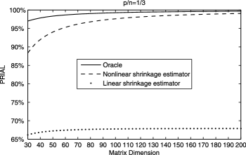
Figure 2: Comparison of the nonlinear vs. linear shrinkage estimators. $20\%$ of population eigenvalues are equal to $1$, $40\%$ are equal to $3$ and $40\%$ are equal to $10$. Every point is the result of $1000$ Monte Carlo simulations.

One can see that the performance of the nonlinear shrinkage estimator $\widehat{S}_{n}$ converges quickly toward that of the oracle and of $S^{*}_{n}$. Even for relatively small matrices of dimension $p=30$, it realizes $88\%$ of the possible gains over the sample covariance matrix. The optimal linear shrinkage estimator $\overline{S}_{n}$ also performs well relative to the sample covariance matrix, but the improvement is limited: in general, it does not converge to $100\%$ under large-dimensional asymptotics. This is because there are strong nonlinear effects in the optimal shrinkage of sample eigenvalues. These effects are clearly visible in Figure 3, which plots a typical simulation result for $p=100$.

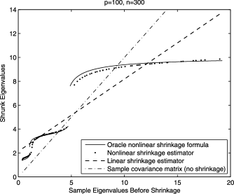
Figure 3: Nonlinearity of the oracle shrinkage formula. $20\%$ of population eigenvalues are equal to $1$, $40\%$ are equal to $3$ and $40\%$ are equal to $10$. $p=100$ and $n=300$.

One can see that the nonlinear shrinkage estimator $\widehat{S}_{n}$ shrinks the eigenvalues of the sample covariance matrix almost as if it “knew” the correct shape of the distribution of population eigenvalues. In particular, the various curves and gaps of the oracle nonlinear shrinkage formula are well picked up and followed by this estimator. By contrast, the linear shrinkage estimator can only use the best linear approximation to this highly nonlinear transformation. We also plot the $45$-degrees line as a visual reference to show what would happen if no shrinkage was applied to the sample eigenvalues, that is, if we simply used $S_{n}$.

6.2 Concentration

The next set of Monte Carlo simulations shows how the PRIAL of the shrinkage estimators varies as a function of the concentration ratio $\widehat{c}_{n}=p/n$ if we keep the product $p\times n$ constant and equal to $9000$. We keep the same population covariance matrix $\Sigma_{n}$ as in Section 6.1. For every value of $p/n$, we run $1000$ simulations with normally distributed variables. The respective PRIALs of $S_{n}^{or}$, $\widehat{S}_{n}$ and $\overline{S}_{n}$ are plotted in Figure 4.

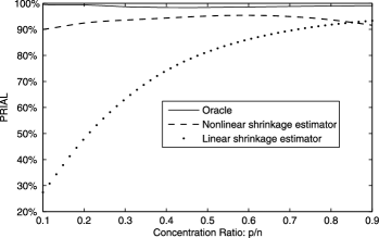
Figure 4: Effect of varying the concentration ratio $\widehat{c}_{n}=p/n$. $20\%$ of population eigenvalues are equal to $1$, $40\%$ are equal to $3$ and $40\%$ are equal to $10$. Every point is the result of $1000$ Monte Carlo simulations.

One can see that the nonlinear shrinkage estimator performs well across the board, closely in line with the oracle, and always achieves at least $90\%$ of the possible improvement over the sample covariance matrix. By contrast, the linear shrinkage estimator achieves relatively little improvement over the sample covariance matrix when the concentration is low. This is because, when the sample size is large relative to the matrix dimension, there is a lot of precise information about the optimal nonlinear way to shrink the sample eigenvalues that is waiting to be extracted by a suitable nonlinear procedure. By contrast, when the sample size is not so large, the information about the population covariance matrix is relatively fuzzy; therefore a simple linear approximation can achieve up to $93\%$ of the potential gains.

6.3 Dispersion

The third set of Monte Carlo simulations shows how the PRIAL of the shrinkage estimators varies as a function of the dispersion of population eigenvalues. We take a population covariance matrix $\Sigma_{n}$ with $20\%$ of its eigenvalues equal to $1$, $40\%$ equal to $1+2d/9$ and $40\%$ equal to $1+d$, where the dispersion parameter $d$ varies from $0$ to $20$. Thus, for $d=0$, $\Sigma_{n}$ is the identity matrix and, for $d=9$, $\Sigma_{n}$ is the same matrix as in Section 6.1. The sample size is $n=300$ and the matrix dimension is $p=100$. For every value of $d$, we run $1000$ simulations with normally distributed variables. The respective PRIALs of $S_{n}^{or}$, $\widehat{S}_{n}$ and $\overline{S}_{n}$ are plotted in Figure 5.

Figure 5: Effect of varying the dispersion of population eigenvalues. $20\%$ of population eigenvalues are equal to $1$, $40\%$ equal to $1+2d/9$ and $40\%$ equal to $1+d$, where the dispersion parameter $d$ varies from $0$ to $20$. $p=100$ and $n=300$. Every point is the result of $1000$ Monte Carlo simulations.

One can see that the linear shrinkage estimator $\overline{S}_{n}$ beats the nonlinear shrinkage estimator $\widehat{S}_{n}$ for very low dispersion levels. For example, when $d=0$, that is, when the population covariance matrix is equal to the identity matrix, $\overline{S}_{n}$ realizes $99.9\%$ of the possible improvement over the sample covariance matrix, while $\widehat{S}_{n}$ realizes “only” $99.4\%$ of the possible improvement. This is because, in this case, linear shrinkage is optimal or (when $d$ is strictly positive but still small) nearly optimal Hence there is nothing too little to be gained by resorting to a nonlinear shrinkage method. However, as dispersion increases, linear shrinkage delivers less and less improvement over the sample covariance matrix, while nonlinear shrinkage retains a PRIAL above $96\%$, and close to that of the oracle.

6.4 Fat tails

We also have some results on the effect of non-normality on the performance of the shrinkage estimators. We take the same population covariance matrix as in Section 6.1, that is, $\Sigma_{n}$ has $20\%$ of its eigenvalues equal to $1$, $40\%$ equal to $3$ and $40\%$ equal to $10$. The sample size is $n=300$, and the matrix dimension is $p=100$. We compare two types of random variates: a Student $t$ distribution with $\mathrm{df}=3$ degrees of freedom, and a Student $t$ distribution with $\mathrm{df}=\infty$ degrees of freedom (which is the Gaussian distribution). For each number of degrees of freedom $\mathrm{df}$, we run $1000$ simulations. The respective PRIALs of $S_{n}^{or}$, $\widehat{S}_{n}$ and $\overline{S}_{n}$ are summarized in Table 1.

==0pt Average squared PRIAL Frobenius loss $\mathbf{df}\bm{=3}$ $\mathbf{df}\bm{=\infty}$ $\mathbf{df}\bm{=3}$ $\mathbf{df}\bm{=\infty}$ Sample covariance matrix 5.856 5.837 0%.0 0%.0 Linear shrinkage estimator 1.883 1.883 67.84% 67.74% Nonlinear shrinkage estimator 0.128 0.133 97.81% 97.71% Oracle 0.043 0.041 99.27% 99.30%

Table 1: Effect of nonnormality. $20\%$ of population eigenvalues are equal to $1$, $40\%$ are equal to $3$ and $40\%$ are equal to $10$. $1000$ Monte Carlo simulations with $p=100$ and $n=300$

One can see that departure from normality does not have any noticeable effect on performance.

6.5 Precision matrix

The next set of Monte Carlo simulations focuses on estimating the precision matrix $\Sigma_{n}^{-1}$. The definition of the PRIAL, in this subsection only, is given by

$$\mathrm{PRIAL}\equiv\mathrm{PRIAL}(\widehat{\Pi}_{n})\equiv 100\times\biggl{\{}1-\frac{{\mathbb{E}}[\|\widehat{\Pi}_{n}-P^{*}_{n}\|^{2}]}{{\mathbb{E}}[\|S_{n}^{-1}-P^{*}_{n}\|^{2}]}\biggr{\}}\%,$$ (44)

where $\widehat{\Pi}_{n}$ is an arbitrary estimator of $\Sigma_{n}^{-1}$. By definition, the PRIAL of $S_{n}^{-1}$ is 0% while the PRIAL of $P_{n}^{*}$ is 100%.

We take the same population eigenvalues as in Section 6.1. The concentration ratio $\widehat{c}_{n}=p/n$ is set to the value $1/3$. For various values of $p$ between $30$ and $200$, we run 1000 simulations with normally distributed variables. The respective PRIALs of $P_{n}^{or}$, $\widehat{P}_{n}$, $\widehat{S}_{n}^{-1}$ and $\overline{S}_{n}^{-1}$ are plotted in Figure 6.

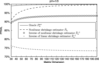
Figure 6: Estimating the precision matrix. $20\%$ of population eigenvalues are equal to $1$, $40\%$ are equal to $3$ and $40\%$ are equal to $10$. Every point is the result of $1000$ Monte Carlo simulations.

One can see that the nonlinear shrinkage method seems to be just as effective for the purpose of estimating the precision matrix as it is for the purpose of estimating the covariance matrix itself. Moreover, there is a clear benefit in directly estimating the precision matrix by means of $\widehat{P}_{n}$ as opposed to the indirect estimation by means of $\widehat{S}_{n}^{-1}$ (which on its own significantly outperforms $\overline{S}_{n}^{-1}$).

6.6 Shape

Next, we study how the nonlinear shrinkage estimator $\widehat{S}_{n}$ performs for a wide variety of shapes of population spectral densities. This requires using a family of distributions with bounded support and which, for various parameter values, can take on different shapes. The best-suited family for this purpose is the beta distribution. The c.d.f. of the beta distribution with parameters $(\alpha,\beta)$ is

$$\forall x\in[0,1]\qquad F_{(\alpha,\beta)}(x)=\frac{\Gamma(\alpha+\beta)}{\Gamma(\alpha)\Gamma(\beta)}\int_{0}^{x}t^{\alpha-1}(1-t)^{\beta-1}\,dt.$$

While the support of the beta distribution is $[0,1]$, we shift it to the interval $[1,10]$ by applying a linear transformation. Thanks to the flexibility of the beta family of densities, selecting different parameters $(\alpha,\beta)$ enables us to generate eight different shapes for the population spectral density: rectangular $(1,1)$, linearly decreasing triangle $(1,2)$, linearly increasing triangle $(2,1)$, circular $(1.5,1.5)$, U-shaped $(0.5,0.5)$, bell-shaped $(5,5)$, left-skewed $(5,2)$ and right-skewed $(2,5)$; see Figure 7 for a graphical illustration.

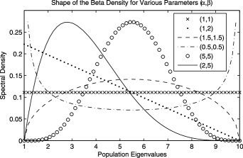
Figure 7: Shape of the beta density for various parameter values. The support of the beta density has been shifted to the interval $[1,10]$ by a linear transformation. To enhance clarity, the densities corresponding to the parameters $(2,1)$ and $(5,2)$ have been omitted, since they are symmetric to $(1,2)$ and $(2,5)$, respectively, about the mid-point of the support.

For every one of these eight beta densities, we take the population eigenvalues to be equal to

$$1+9F_{(\alpha,\beta)}^{-1}\biggl{(}\frac{i}{p}-\frac{1}{2p}\biggr{)},\qquad i=1,\ldots,p.$$

The concentration ratio $\widehat{c}_{n}=p/n$ is equal to $1/3$. For various values of $p$ between $30$ and $200$, we run $1000$ simulations with normally distributed variables. The PRIAL of the nonlinear shrinkage estimator $\widehat{S}_{n}$ is plotted in Figure 8.

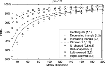
Figure 8: Performance of the nonlinear shrinkage with beta densities. The various curves correspond to different shapes of the population spectral density. The support of the population spectral density is $[1,10]$.

As in all the other simulations presented above, the PRIAL of the nonlinear shrinkage estimator always exceeds $88\%$, and more often than not exceeds $95\%$. To preserve the clarity of the picture, we do not report the PRIALs of the oracle and of the linear shrinkage estimator; but as usual, the nonlinear shrinkage estimator ranked between them.

6.7 Fixed-dimension asymptotics

Finally, we report a set of Monte Carlo simulations that departs from the large-dimensional asymptotics assumption under which the nonlinear shrinkage estimator $\widehat{S}_{n}$ was derived. The goal is to compare it against the sample covariance matrix $S_{n}$ in the setting where $S_{n}$ is known to have certain optimality properties (at least in the normal case): traditional asymptotics, that is, when the number of variables $p$ remains fixed while the sample size $n$ goes to infinity. This gives as much advantage to the sample covariance matrix as it can possibly have. We fix the dimension $p=100$ and let the sample size $n$ vary from $n=125$ to $n=10\mbox{,}000$. In practice, very few applied researchers are fortunate enough to have as many as $n=10\mbox{,}000$ i.i.d. observations, or a concentration ratio $c=p/n$ as low as $0.01$. The respective PRIALs of $S_{n}^{or}$, $\widehat{S}_{n}$ and $\overline{S}_{n}$ are plotted in Figure 9.

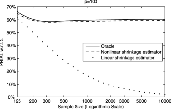
Figure 9: Fixed-dimension asymptotics. $20\%$ of population eigenvalues are equal to $1$, $40\%$ are equal to $3$ and $40\%$ are equal to $10$. Variables are normally distributed. Every point is the result of $1000$ Monte Carlo simulations.

One crucial difference with all the previous simulations is that the target for the PRIAL is no longer $S_{n}^{*}$, but instead the population covariance matrix $\Sigma$ itself, because now $\Sigma$ can be consistently estimated. Note that, since the matrix dimension is fixed, $\Sigma_{n}$ does not change with $n$; therefore, we can drop the subscript $n$. Thus, in this subsection only, the definition of the PRIAL is given by

$$\mathrm{PRIAL}\equiv\mathrm{PRIAL}(\widehat{\Sigma}_{n})\equiv 100\times\biggl{\{}1-\frac{{\mathbb{E}}[\|\widehat{\Sigma}_{n}-\Sigma\|^{2}]}{{\mathbb{E}}[\|S_{n}-\Sigma\|^{2}]}\biggr{\}}\%,$$

where $\widehat{\Sigma}_{n}$ is an arbitrary estimator of $\Sigma$. By definition, the PRIAL of $S_{n}$ is 0% while the PRIAL of $\Sigma$ is 100%.

In this setting, Ledoit and Wolf (2004) acknowledge that the improvement of the linear shrinkage estimator over the sample covariance matrix vanishes asymptotically, because the optimal linear shrinkage intensity vanishes. Therefore it should be no surprise that the PRIAL of $\overline{S}_{n}$ goes to zero in Figure 9. Perhaps more surprising is the continued ability of the oracle and the nonlinear shrinkage estimator to improve by approximately $60\%$ over the sample covariance matrix, even for a sample size as large as $n=10\mbox{,}000$, and with no sign of abating as $n$ goes to infinity. This is an encouraging result, as our simulation gave every possible advantage to the sample covariance matrix by placing it in the asymptotic conditions where it possesses well-known optimality properties, and where the earlier linear shrinkage estimator of Ledoit and Wolf (2004) is most disadvantaged.

Intuitively, this is because the oracle shrinkage formula becomes more and more nonlinear as $n$ goes to infinity for fixed $p$. Bai and Silverstein (1998) show that the sample covariance matrix exhibits “spectral separation” when the concentration ratio $p/n$ is sufficiently small. It means that the sample eigenvalues coalesce into clusters, each cluster corresponding to a Dirac of population eigenvalues. Within a given cluster, the smallest sample eigenvalues need to be nudged upward, and the largest ones downward, to the average of the cluster. In other words: full shrinkage within clusters, and no shrinkage between clusters. This is illustrated in Figure 10, which plots a typical simulation result for $n=10\mbox{,}000$.

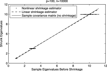
Figure 10: Nonlinear shrinkage under fixed-dimension aymptotics. $20\%$ of population eigenvalues are equal to $1$, $40\%$ are equal to $3$ and $40\%$ are equal to $10$. $p=100$ and $n=10\mbox{,}000$. The oracle is not shown because it is virtually identical to the nonlinear shrinkage estimator.

By detecting this intricate pattern automatically, that is, by discovering where to shrink and where not to shrink, the nonlinear shrinkage estimator $\widehat{S}_{n}$ showcases its ability to generate substantial improvements over the sample covariance matrix even for very low concentration ratios.

6.8 Additional Monte Carlo simulations

6.8.1 Comparisons with other estimators

So far, we have compared the nonlinear shrinkage estimator $\widehat{S}_{n}$ only to the linear shrinkage estimator $\overline{S}_{n}$ and the oracle estimator $S_{n}^{or}$ to keep the resulting figures concise and legible.

It is of additional interest to compare the nonlinear shrinkage estimator also to some other estimators from the literature. To this end we consider the following set of estimators:

• The estimator of Stein (1975);

• The estimator of Haff (1980);

• The estimator recently proposed by Won et al. (2009). This estimator is based on a maximum likelihood approach, assuming normality, with an explicit constraint on the condition number of the covariance matrix. The resulting estimator turns out to be a nonlinear shrinkage estimator as well: all “small” sample eigenvalues are brought up to a lower bound, all “large” sample eigenvalues are brought down to an upper bound, and all “intermediate” sample eigenvalues are left unchanged.

  Therefore, the corresponding transformation from sample eigenvalues to shrunk eigenvalues is step-wise linear: first flat, then a 45-degree line, and then flat again. The upper and lower bounds are determined by the desired constraint on the condition number $\kappa$. If such an explicit constraint is not available from a priori information, a suitable constraint number $\widehat{\kappa}$ can be computed in a data-dependent fashion by a $K$-fold cross-validation method, which is the method we use.

  In particular, the cross-validation method selects $\widehat{\kappa}$ by optimizing over a finite grid $\{\kappa_{1},\kappa_{2},\ldots,\kappa_{L}\}$ that has to be supplied by the user. To this end we choose $L=10$ and the $\kappa_{l}$ log-linearly spaced between 1 and $\kappa(S_{n})$, for $l=1,\ldots,L$; here $\kappa(S_{n})$ denotes the condition number of the sample covariance matrix. More precisely, for $l=1,\ldots,L$, $\kappa_{l}\equiv\exp(\omega_{l})$, where $\{\omega_{1},\omega_{2},\ldots,\omega_{L}\}$ is the equally-spaced grid with $\omega_{1}\equiv 0$ and $\omega_{L}\equiv\log(\kappa(S_{n}))$.

• The cross-validation version of the nonlinear shrinkage estimator $\widehat{S}_{n}$; see Remark 5.2.

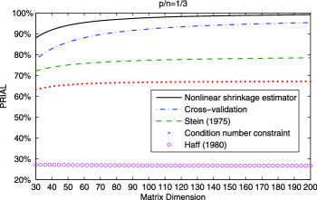
Figure 11: Comparison of various estimators. $20\%$ of population eigenvalues are equal to $1$, $40\%$ are equal to $3$ and $40\%$ are equal to $10$. Every point is the result of $1000$ Monte Carlo simulations.

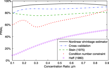
Figure 12: Effect of varying the concentration ratio $\widehat{c}_{n}=p/n$. $20\%$ of population eigenvalues are equal to $1$, $40\%$ are equal to $3$ and $40\%$ are equal to $10$. Every point is the result of $1000$ Monte Carlo simulations.

We repeat the simulation exercises of Sections 6.1–6.3, replacing the oracle estimator and the linear shrinkage estimator with the above set of other estimators. The respective PRIALs of the various estimators are plotted in Figures 11–13.

One can see that the nonlinear shrinkage estimator $\widehat{S}_{n}$ outperforms all other estimators, with the cross-validation version of $\widehat{S}_{n}$ in second place, followed by the estimators of Stein (1975), Won et al. (2009) and Haff (1980).

6.8.2 Comparisons based on a different loss function

So far, the PRIAL has been based on the loss function

$$L^{Fr}(\widehat{\Sigma}_{n},\Sigma_{n})\equiv\|\widehat{\Sigma}_{n}-\Sigma_{n}\|^{2}.$$

It is of additional interest to add some comparisons based on a different loss function. To this end we use the scale-invariant loss function proposed by James and Stein (1961), namely

$$L^{JS}(\widehat{\Sigma}_{n},\Sigma_{n})\equiv\operatorname{trace}(\widehat{\Sigma}_{n}\Sigma_{n}^{-1})-\log\det(\widehat{\Sigma}_{n}\Sigma_{n}^{-1})-p.$$ (45)

We repeat the simulation exercises of Sections 6.1–6.3, replacing $L^{Fr}$ with $L^{JS}$. The respective PRIALs of $S_{n}^{or}$, $\widehat{S}_{n}$, and $\overline{S}_{n}$ are plotted in Figures 14–16.

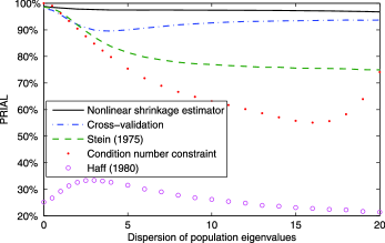
Figure 13: Effect of varying the dispersion of population eigenvalues. $20\%$ of population eigenvalues are equal to $1$, $40\%$ equal to $1+2d/9$ and $40\%$ equal to $1+d$, where the dispersion parameter $d$ varies from $0$ to $20$. $p=100$ and $n=300$. Every point is the result of $1000$ Monte Carlo simulations.

One can see that the results do not change much qualitatively. If anything, the comparisons are now even more favorable to the nonlinear shrinkage estimator, in particular when comparing Figure 5 to Figure 16.

Figure 14: Comparison of the nonlinear vs. linear shrinkage estimators. $20\%$ of population eigenvalues are equal to $1$, $40\%$ are equal to $3$ and $40\%$ are equal to $10$. The PRIALs are based on the James–Stein (1961) loss function (45). Every point is the result of $1000$ Monte Carlo simulations.

Figure 15: Effect of varying the concentration ratio $\widehat{c}_{n}=p/n$. $20\%$ of population eigenvalues are equal to $1$, $40\%$ are equal to $3$ and $40\%$ are equal to $10$. The PRIALs are based on the James–Stein (1961) loss function (45). Every point is the result of $1000$ Monte Carlo simulations.

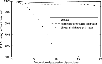
Figure 16: Effect of varying the dispersion of population eigenvalues. $20\%$ of population eigenvalues are equal to $1$, $40\%$ equal to $1+2d/9$ and $40\%$ equal to $1+d$, where the dispersion parameter $d$ varies from $0$ to $20$. $p=100$ and $n=300$. The PRIALs are based on the James and Stein (1961) loss function (45). Every point is the result of $1000$ Monte Carlo simulations.

7 Conclusion

Estimating a large-dimensional covariance matrix is a very important and challenging problem. In the absence of additional information concerning the structure of the true covariance matrix, a successful approach consists of appropriately shrinking the sample eigenvalues, while retaining the sample eigenvectors. In particular, such shrinkage estimators enjoy the desirable property of being rotation-equivariant.

In this paper, we have extended the linear approach of Ledoit and Wolf (2004) by applying a nonlinear transformation to the sample eigenvalues. The specific transformation suggested is motivated by the oracle estimator of Ledoit and Péché (2011), which in turn was derived by studying the asymptotic behavior of the finite-sample optimal rotation-equivariant estimator (i.e., the estimator with the rotation-equivariant property that is closest to the true covariance matrix when distance is measured by the Frobenius norm).

The oracle estimator involves the Stieltjes transform of the limiting spectral distribution of the sample eigenvalues, evaluated at various points on the real line. By finding a way to consistently estimate these quantities, in a uniform sense, we have been able to construct a bona fide nonlinear shrinkage estimator that is asymptotically equivalent to the oracle.

Extensive Monte Carlo studies have demonstrated the improved finite-sample properties of our nonlinear shrinkage estimator compared to the sample covariance matrix and the linear shrinkage estimator of Ledoit and Wolf (2004), as well as its fast convergence to the performance of the oracle. In particular, when the sample size is very large compared to the dimension, or the population eigenvalues are very dispersed, the nonlinear shrinkage estimator still yields a significant improvement over the sample covariance matrix, while the linear shrinkage estimator no longer does.

Many statistical applications require an estimator of the inverse of the covariance matrix, which is called the precision matrix. We have modified our nonlinear shrinkage approach to this alternative problem, thereby constructing a direct estimator of the precision matrix. Monte Carlo studies have confirmed that this estimator yields a sizable improvement over the indirect method of simply inverting the nonlinear shrinkage estimator of the covariance matrix itself.

The scope of this paper is limited to the case where the matrix dimension is smaller than the sample size. The other case, where the matrix dimension exceeds the sample size, requires certain modifications in the mathematical treatment, and is left for future research.

References

- Bai and Silverstein (1998) {barticle}[mr] \bauthor\bsnmBai, \bfnmZ. D.\binitsZ. D. and \bauthor\bsnmSilverstein, \bfnmJack W.\binitsJ. W. (\byear1998). \btitleNo eigenvalues outside the support of the limiting spectral distribution of large-dimensional sample covariance matrices. \bjournalAnn. Probab. \bvolume26 \bpages316–345. \biddoi=10.1214/aop/1022855421, issn=0091-1798, mr=1617051 \bptokimsref \endbibitem
- Bickel and Levina (2008) {barticle}[mr] \bauthor\bsnmBickel, \bfnmPeter J.\binitsP. J. and \bauthor\bsnmLevina, \bfnmElizaveta\binitsE. (\byear2008). \btitleRegularized estimation of large covariance matrices. \bjournalAnn. Statist. \bvolume36 \bpages199–227. \biddoi=10.1214/009053607000000758, issn=0090-5364, mr=2387969 \bptokimsref \endbibitem
- Cai and Zhou (2012) {bmisc}[author] \bauthor\bsnmCai, \bfnmT.\binitsT. and \bauthor\bsnmZhou, \bfnmH.\binitsH. (\byear2012). \bhowpublishedMinimax estimation of large covariance matrices under norm. Statist. Sinica. To appear. \bptokimsref \endbibitem
- El Karoui (2008) {barticle}[mr] \bauthor\bsnmEl Karoui, \bfnmNoureddine\binitsN. (\byear2008). \btitleSpectrum estimation for large dimensional covariance matrices using random matrix theory. \bjournalAnn. Statist. \bvolume36 \bpages2757–2790. \biddoi=10.1214/07-AOS581, issn=0090-5364, mr=2485012 \bptokimsref \endbibitem
- Fan, Fan and Lv (2008) {barticle}[mr] \bauthor\bsnmFan, \bfnmJianqing\binitsJ., \bauthor\bsnmFan, \bfnmYingying\binitsY. and \bauthor\bsnmLv, \bfnmJinchi\binitsJ. (\byear2008). \btitleHigh dimensional covariance matrix estimation using a factor model. \bjournalJ. Econometrics \bvolume147 \bpages186–197. \biddoi=10.1016/j.jeconom.2008.09.017, issn=0304-4076, mr=2472991 \bptokimsref \endbibitem
- Gill, Murray and Saunders (2002) {barticle}[mr] \bauthor\bsnmGill, \bfnmPhilip E.\binitsP. E., \bauthor\bsnmMurray, \bfnmWalter\binitsW. and \bauthor\bsnmSaunders, \bfnmMichael A.\binitsM. A. (\byear2002). \btitleSNOPT: An SQP algorithm for large-scale constrained optimization. \bjournalSIAM J. Optim. \bvolume12 \bpages979–1006 (electronic). \biddoi=10.1137/S1052623499350013, issn=1052-6234, mr=1922505 \bptokimsref \endbibitem
- Haff (1980) {barticle}[mr] \bauthor\bsnmHaff, \bfnmL. R.\binitsL. R. (\byear1980). \btitleEmpirical Bayes estimation of the multivariate normal covariance matrix. \bjournalAnn. Statist. \bvolume8 \bpages586–597. \bidissn=0090-5364, mr=0568722 \bptokimsref \endbibitem
- James and Stein (1961) {bincollection}[mr] \bauthor\bsnmJames, \bfnmW.\binitsW. and \bauthor\bsnmStein, \bfnmCharles\binitsC. (\byear1961). \btitleEstimation with quadratic loss. In \bbooktitleProc. 4th Berkeley Sympos. Math. Statist. and Prob., Vol. I \bpages361–379. \bpublisherUniv. California Press, \baddressBerkeley, Calif. \bidmr=0133191 \bptokimsref \endbibitem
- Khare and Rajaratnam (2011) {barticle}[mr] \bauthor\bsnmKhare, \bfnmKshitij\binitsK. and \bauthor\bsnmRajaratnam, \bfnmBala\binitsB. (\byear2011). \btitleWishart distributions for decomposable covariance graph models. \bjournalAnn. Statist. \bvolume39 \bpages514–555. \biddoi=10.1214/10-AOS841, issn=0090-5364, mr=2797855 \bptokimsref \endbibitem
- Ledoit and Péché (2011) {barticle}[mr] \bauthor\bsnmLedoit, \bfnmOlivier\binitsO. and \bauthor\bsnmPéché, \bfnmSandrine\binitsS. (\byear2011). \btitleEigenvectors of some large sample covariance matrix ensembles. \bjournalProbab. Theory Related Fields \bvolume151 \bpages233–264. \biddoi=10.1007/s00440-010-0298-3, issn=0178-8051, mr=2834718 \bptokimsref \endbibitem
- Ledoit and Wolf (2004) {barticle}[mr] \bauthor\bsnmLedoit, \bfnmOlivier\binitsO. and \bauthor\bsnmWolf, \bfnmMichael\binitsM. (\byear2004). \btitleA well-conditioned estimator for large-dimensional covariance matrices. \bjournalJ. Multivariate Anal. \bvolume88 \bpages365–411. \biddoi=10.1016/S0047-259X(03)00096-4, issn=0047-259X, mr=2026339 \bptokimsref \endbibitem
- Ledoit and Wolf (2012) {bmisc}[author] \bauthor\bsnmLedoit, \bfnmO.\binitsO. and \bauthor\bsnmWolf, \bfnmM.\binitsM. (\byear2012). \bhowpublishedSupplement to “Nonlinear shrinkage estimation of large-dimensional covariance matrices.” DOI:\doiurl10.1214/12-AOS989SUPP. \bptokimsref \endbibitem