Spontaneous Circulation of Confined Active Suspensions

Abstract

Many active fluid systems encountered in biology are set in total geometric confinement. Cytoplasmic streaming in plant cells is a prominent and ubiquitous example, in which cargo-carrying molecular motors move along polymer filaments and generate coherent cell-scale flow. When filaments are not fixed to the cell periphery, a situation found both in vivo and in vitro, we observe that the basic dynamics of streaming are closely related to those of a non-motile stresslet suspension. Under this model, it is demonstrated that confinement makes possible a stable circulating state; a linear stability analysis reveals an activity threshold for spontaneous auto-circulation. Numerical analysis of the long-time behavior reveals a phenomenon akin to defect separation in nematic liquid crystals, and a high-activity bifurcation to an oscillatory regime.

Cytoplasmic streaming is the deliberate, driven motion of the entire contents of large eukaryotic cells. It is effected by cargo-laden molecular motors walking along polymer filaments and entraining the surrounding fluid (Fig. 1a); the combined action of many of these motors can generate flow speeds in excess of $100$ $\mathrm{\mu m/s}$ for certain freshwater algae. While inroads are being made into understanding its function Protoplasma ; Goldstein2008 , surprisingly little is known about how it is initially established within cells.

In a remarkable, yet apparently little-known investigation into the development of streaming, Yotsuyanagi Yotsuyanagi in 1953 examined isolated droplets of cytoplasm forcibly extracted from algal cells. He observed a progression from isolated Brownian fluctuations to a coherent, global circulation of the entire droplet contents (Fig. 1b). However, we need not limit ourselves to ex vivo experiments: Kamiya Kamiya1959 describes a similar blooming of rotational cyclosis in the development of Lilium pollen cells, and Jarosch Jarosch1956 quantitatively analyzed the same disorder-to-order transition occurring within Allium cells over the course of a few hours. Based on these observations, one is led to ask: is it possible that a simple self-organization process could lie at the heart of streaming?

When the filaments are not locked in position, as is likely in Yotsuyanagi’s experiments, a cargo-carrying motor walking on a free filament constitutes a force dipole. Therefore, these cytoplasmic dynamics belong to the burgeoning field of active fluids. With roots in self-organizing flocking models Flocking , an active fluid is a suspension of force dipoles interacting via short- and long-range forces: a system like a liquid crystal but with continuous injection of energy at the microscale. Such systems generically possess spontaneous flow instabilities SimhaRamaswamy2002 and can exhibit complex patterns and flows Voituriez2005 , including asters and vortices Kruse2004 ; Elgeti2011 ; Kruse2005 , laning GiomiMarchetti2011 ; Giomi and density waves Kruse2005 ; GiomiMarchetti2011 ; Giomi . Spontaneous flow in particular is a key characteristic of flocking dynamics Flocking , and assumes an important role in applications such as cortex remodeling processes Salbreux2008 .

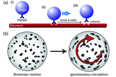
Figure 1: (color online). Cytoplasmic streaming in vivo and ex vivo. (a) A molecular motor attached to a vesicle (i) encounters a filament, (ii) binds and walks along it, entraining fluid, before (iii) unbinding stochastically. (b) A drop of cytoplasm extracted from a plant cell transitions from random Brownian fluctuations to ordered circulation Yotsuyanagi .

Despite the ubiquity of relevant situations, of which streaming is a major example, the influence of total confinement is relatively little-studied. Kruse et al. Kruse2004 included a finite domain in their study of single defect stability in polar gels, assuming perfect alignment everywhere bar the defect core, and found a dependence of aster and vortex stability on domain size. More recently, Schaller et al. Schaller2010 underlined the critical importance of long-range hydrodynamics in confined systems: swirling patterns were observed experimentally in a totally confined actin motility assay, but were absent in cellular automaton simulations. They concluded that confined flows are responsible for the formation and stability of the global circulation. It seems reasonable, therefore, to posit that combining confinement with the spontaneous flow characteristics of active fluids will lead to circulatory streaming states. Indeed, such effects were taken advantage of by Fürthauer et al. Furthauer2012 to construct theoretically a ‘Taylor–Couette motor’, albeit in a geometry topologically distinct from a single confined chamber.

Through theory and simulation, we show here that the combination of confinement and activity allows for the emergence of stable self-organized rotational streaming. This is achieved using a ground-up approach employing closure techniques new to active suspension theory. Our model assumes that short, rigid filaments are suspended in a Newtonian, zero Reynolds number fluid, and they exert extensile, or ‘pusher’, dipolar forces on the fluid; this can be viewed as the effect of processive molecular motors landing randomly along a filament and walking toward one end, implying an average motor location forward of the filament midpoint. The suspension is taken to be dilute, so filaments interact via hydrodynamics only, and is confined within a no-slip sphere of diameter $L$.

Working in $d$ dimensions we generalize the standard kinetic approach to these systems SaintillanShelley . The spatial and angular distribution function $\Psi({\mathbf{x}},{\mathbf{p}},t)$ of the filaments, where $|{\mathbf{p}}|=1$, satisfies a Smoluchowski equation

$$\frac{\partial\Psi}{\partial t}=-{\bm{\nabla}}_{\mathbf{x}}\cdot(\dot{\mathbf{x}}\Psi)-{\bm{\nabla}}_{\mathbf{p}}\cdot(\dot{\mathbf{p}}\Psi)$$ (1)

where ${\bm{\nabla}}_{\mathbf{x}}\equiv\partial/\partial{\mathbf{x}}$ and ${\bm{\nabla}}_{\mathbf{p}}\equiv({\mathbf{{I}}}-{\mathbf{p}}{\mathbf{p}})\cdot\partial/\partial{\mathbf{p}}$. The spatial and rotational fluxes are

$$\dot{\mathbf{x}} \equiv{\mathbf{u}}+V{\mathbf{p}}-{\bm{\mathsf{D}}}^{(s)}\cdot{\bm{\nabla}}_{\mathbf{x}}\log\Psi,$$

$$\dot{\mathbf{p}} \equiv({\mathbf{{I}}}-{\mathbf{p}}{\mathbf{p}})\cdot(\gamma{\bm{\mathsf{E}}}+{\bm{\mathsf{W}}})\cdot{\mathbf{p}}-D^{(r)}{\bm{\nabla}}_{\mathbf{p}}\log\Psi,$$

where $V$ is a self-advection speed, $\gamma\in[-1,1]$ is a shape parameter ($\gamma\rightarrow 1$ for a slender rod), ${\bm{\mathsf{D}}}^{(s)}$ is a spatial diffusion tensor and $D^{(r)}$ is a rotational diffusion constant. The fluid has velocity field ${\mathbf{u}}$, rate-of-strain tensor ${\bm{\mathsf{E}}}\equiv({\bm{\nabla}}{\mathbf{u}}+{\bm{\nabla}}{\mathbf{u}}^{\mathsf{T}})/2$ and vorticity tensor ${\bm{\mathsf{W}}}\equiv({\bm{\nabla}}{\mathbf{u}}-{\bm{\nabla}}{\mathbf{u}}^{\mathsf{T}})/2$. The filament pusher stresslet of strength $\sigma>0$ generates a stress tensor ${\bm{\Sigma}}\equiv-\sigma\int_{\mathbf{p}}d{\mathbf{p}}\,({\mathbf{p}}{\mathbf{p}}-{\mathbf{{I}}}/d)\Psi$ that drives fluid flow by the Stokes equation $-\mu\nabla^{2}{\mathbf{u}}+{\bm{\nabla}}\Pi={\bm{\nabla}}\cdot{\bm{\Sigma}}$ with viscosity $\mu$ and pressure $\Pi$, subject to incompressibility $\quad{\bm{\nabla}}\cdot{\mathbf{u}}=0$. Confinement induces the no-slip boundary condition ${\mathbf{u}}=0$ on $|{\mathbf{x}}|=L/2$.

While simulations of the full system (1) are possible SaintillanShelley ; HelzelOtto2006 ; PahlavanSaintillan2011 , here we develop evolution equations for the primary orientation moments DoiEdwards1988 ; DeGennesProst1995 ; BaskaranMarchetti2008 . Given the orientational average $\langle\phi\rangle\equiv\int_{\mathbf{p}}d{\mathbf{p}}\,\phi\Psi$, define the concentration $c\equiv\langle 1\rangle$, polar moment ${\mathbf{P}}\equiv\langle{\mathbf{p}}\rangle$ and nematic moment ${\bm{\mathsf{Q}}}\equiv\langle{\mathbf{p}}{\mathbf{p}}-{\mathbf{{I}}}/d\rangle$. Equations of motion for these fields in terms of higher moments can then be derived by taking appropriate weighted integrals of Eq. (1) WoodhouseGoldsteinToAppear .

We pare down complications by specializing to two dimensions ($d=2$), rodlike particles ($\gamma=1$) and isotropic diffusion (${\bm{\mathsf{D}}}^{(s)}=D^{(s)}{\mathbf{{I}}}$), and neglect self-advection ($V\equiv 0$). This last assumption decouples the $c$ dynamics into pure advection-diffusion and eliminates all polar interactions, so we take a constant concentration $c\equiv c_{0}$ and neglect ${\mathbf{P}}$. However, the remaining ${\bm{\mathsf{Q}}}$ dynamics still depends on the fourth moment contraction $\langle{\mathbf{p}}{\mathbf{p}}{\mathbf{p}}{\mathbf{p}}\rangle:{\bm{\mathsf{E}}}$, and a closure is needed. Typically this is done by taking the distribution $\Psi$ to be a functional purely of the first three moments, yielding a closure linear in ${\bm{\mathsf{Q}}}$ BaskaranMarchetti2008 . In dense active systems this is permissible, owing to the presence of local interaction terms in higher powers of ${\bm{\mathsf{Q}}}$; here, however, it is the above fourth moment term which provides all stabilizing nonlinearities, so greater care must be taken. Instead we adopt a new approach by adapting a closure of Hinch and Leal HinchLeal1976 to $d=2$, yielding

$$\langle{\mathbf{p}}{\mathbf{p}}{\mathbf{p}}{\mathbf{p}}\rangle:{\bm{\mathsf{E}}}\approx\frac{1}{4c_{0}}\left[4{\bm{\mathsf{Q}}}\cdot{\bm{\mathsf{E}}}\cdot{\bm{\mathsf{Q}}}+2c_{0}({\bm{\mathsf{E}}}\cdot{\bm{\mathsf{Q}}}+{\bm{\mathsf{Q}}}\cdot{\bm{\mathsf{E}}})\right.$$

$$\quad+\left.c_{0}^{2}{\bm{\mathsf{E}}}-2{\mathbf{{I}}}{\bm{\mathsf{Q}}}^{2}:{\bm{\mathsf{E}}}\right].$$

This is derived in HinchLeal1976 as an interpolation between exact closures for the regimes of total order and disorder, giving a simple approximation to the hydrodynamic nonlinearities. After non-dimensionalizing by rescaling ${\mathbf{x}}\rightarrow L{\mathbf{x}}$, $t\rightarrow(c_{0}L^{2}/\mu)t$, ${\mathbf{u}}\rightarrow(\mu/c_{0}L){\mathbf{u}}$, $\Pi\rightarrow(\mu^{2}/c_{0}L^{2})\Pi$, ${\bm{\Sigma}}\rightarrow(c_{0}L^{2}/\mu^{2}){\bm{\Sigma}}$ and ${\bm{\mathsf{Q}}}\rightarrow c_{0}{\bm{\mathsf{Q}}}$, the final model reads

$$\frac{D{\bm{\mathsf{Q}}}}{Dt}=d^{(s)}\nabla^{2}{\bm{\mathsf{Q}}}-4d^{(r)}{\bm{\mathsf{Q}}}+\tfrac{1}{2}{\bm{\mathsf{E}}}-2{\bm{\mathsf{Q}}}\cdot{\bm{\mathsf{E}}}\cdot{\bm{\mathsf{Q}}}$$ (2)

where $D/Dt\equiv\partial/\partial t+{\mathbf{u}}\cdot{\bm{\nabla}}$, with non-dimensional diffusion constants $d^{(s)}\equiv(c_{0}/\mu)D^{(s)}$ and $d^{(r)}\equiv(c_{0}L^{2}/\mu)D^{(r)}$. This is subject to the Stokes equation $-\nabla^{2}{\mathbf{u}}+{\bm{\nabla}}\Pi=-\sigma_{0}{\bm{\nabla}}\cdot{\bm{\mathsf{Q}}}$ and incompressibility ${\bm{\nabla}}\cdot{\mathbf{u}}=0$ with non-dimensional dipole stress $\sigma_{0}\equiv(c_{0}L/\mu)^{2}\sigma$. The fluid boundary condition reads ${\mathbf{u}}=0$ on $|{\mathbf{x}}|=1/2$. Among the variety of admissible boundary conditions on ${\bm{\mathsf{Q}}}$ we focus here on the natural condition ${\mathbf{N}}\cdot{\bm{\nabla}}{\bm{\mathsf{Q}}}=0$, where ${\mathbf{N}}$ is the boundary normal vector. Qualitatively similar results are found with fixed boundary-parallel or boundary-perpendicular conditions WoodhouseGoldsteinToAppear .

The model (2) has the structure of a Landau theory for the order parameter ${\bm{\mathsf{Q}}}$. As ${\bm{\mathsf{E}}}$ is linear in the velocity ${\mathbf{u}}$, and ${\mathbf{u}}$ is (nonlocally) linear in $\sigma_{0}{\bm{\mathsf{Q}}}$ via the Stokes equation, the term $(1/2){\bm{\mathsf{E}}}\propto\sigma_{0}{\bm{\mathsf{Q}}}$. It follows in the usual manner that there is an effective linear term in ${\bm{\mathsf{Q}}}$ that will become positive for sufficiently large activity $\sigma_{0}$ relative to $-4d^{(r)}$. If this is sufficient to overcome the diffusive stabilization $d^{(s)}$ then the amplitude of the ensuing instability will be limited by the nonlinear term $2{\bm{\mathsf{Q}}}\cdot{\bm{\mathsf{E}}}\cdot{\bm{\mathsf{Q}}}\propto{\bm{\mathsf{Q}}}^{3}$.

We first seek a steady non-flowing axisymmetric state ${\bm{\mathsf{Q}}}^{0}$. In polar coordinates $\alpha=(r,\theta)$ the tensor Laplacian of ${\bm{\mathsf{Q}}}$ has primary components

$$(\nabla^{2}{\bm{\mathsf{Q}}})_{r\alpha}={\mathcal{L}}Q_{r\alpha}\equiv\frac{1}{r}\frac{\partial}{\partial r}\left(r\frac{\partial Q_{r\alpha}}{\partial r}\right)-\frac{4}{r^{2}}Q_{r\alpha}~{},$$

while the others follow from symmetry and the tracelessness of ${\bm{\mathsf{Q}}}$. Eq. (2) therefore implies $Q^{0}_{rr}$ and $Q^{0}_{r\theta}$ each satisfy a (modified) Bessel equation in $z\equiv 2\Delta r$, viz. $z^{2}\partial_{z}^{2}Q^{0}_{r\alpha}+z\partial_{z}Q^{0}_{r\alpha}-(z^{2}+4)Q^{0}_{r\alpha}=0$, where $\Delta^{2}\equiv d^{(r)}/d^{(s)}$. Thus $Q^{0}_{r\alpha}\propto I_{2}(2\Delta r)$; since $I_{2}$ is monotonic, the boundary conditions imply ${\bm{\mathsf{Q}}}^{0}=0$ everywhere.

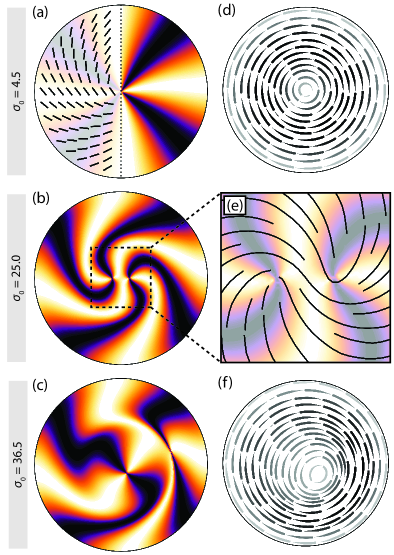
Figure 2: (color online). Numerical results beyond the spontaneous circulation threshold. (a,b,c) Simulated schlieren textures of nematic order director ${\mathbf{n}}$ (i.e. density plot of $(n_{x}n_{y})^{2}$). Lighter corresponds to diagonally-oriented filaments, darker to horizontal or vertical. (a) Steady circulation with a central spiral defect at low activity (left overlay shows order field ${\mathbf{n}}$), (b) steady central defect separation into a pair of hyperbolic defects, (c) snapshot of oscillatory behavior with widely separated mobile defects. (d) Flow streamlines for low activity, showing circulation about the system center; darker streamlines indicate faster flow. (e) Enlargement of nematic director field structure in texture (b), showing two hyperbolic defects. (f) Flow streamlines for high-activity oscillation associated with texture (c) exhibiting off-center flow circulation. In all cases, $d^{(r)}=d^{(s)}=0.025$.

Now, perturb axisymmetrically: let ${\bm{\mathsf{Q}}}=\epsilon{\bm{\mathsf{R}}}$, $\epsilon\ll 1$, and write ${\mathbf{u}}=\epsilon v\hat{\bm{\theta}}$, ${\bm{\mathsf{E}}}=\epsilon{\bm{\mathsf{e}}}$ for the induced flow (which has no radial component by incompressibility). Seek an exponentially growing state such that $\partial_{t}{\bm{\mathsf{R}}}=s{\bm{\mathsf{R}}}$. Then to $O(\epsilon)$, the perturbation obeys $s{\bm{\mathsf{R}}}=d^{(s)}\nabla^{2}{\bm{\mathsf{R}}}-4d^{(r)}{\bm{\mathsf{R}}}+\tfrac{1}{2}{\bm{\mathsf{e}}}$. To determine ${\bm{\mathsf{e}}}$ we employ the technique of Kruse et al. Kruse2004 and write the Stokes equation as ${\bm{\nabla}}\cdot(-\tilde{\Pi}{\mathbf{{I}}}+2{\bm{\mathsf{e}}}-\sigma_{0}{\bm{\mathsf{R}}})\equiv{\bm{\nabla}}\cdot{\bm{\Sigma}}^{\text{tot}}=0$. The $r$-component determines $\Pi$. The $\theta$-component reads $\partial_{r}\Sigma^{\text{tot}}_{r\theta}+(2/r)\Sigma^{\text{tot}}_{r\theta}=0$, so for $\Sigma^{\text{tot}}_{r\theta}$ analytic at $r=0$ we find $\Sigma^{\text{tot}}_{r\theta}=0$, i.e. $e_{r\theta}=(\sigma_{0}/2)R_{r\theta}$. Finally, $e_{rr}=0$ as there is no radial velocity component. The perturbation therefore satisfies

$$d^{(s)}{\mathcal{L}}R_{rr} =(4d^{(r)}+s)R_{rr},$$ (3)

$$d^{(s)}{\mathcal{L}}R_{r\theta} =\left(4d^{(r)}+s-\tfrac{\sigma_{0}}{4}\right)R_{r\theta},$$ (4)

which are still of Bessel form. When $s>-4d^{(r)}$, Eq. (3) has a solution in terms of $I_{2}$, so boundary conditions imply $R_{rr}=0$. Now, let $\lambda\equiv(4d^{(r)}+s-\sigma_{0}/4)/d^{(s)}$ and write Eq. (4) as ${\mathcal{L}}R_{r\theta}=\lambda R_{r\theta}$. For $\lambda>0$ this again gives solutions in terms of $I_{2}$ and so $R_{r\theta}=0$. However, for $\lambda<0$ (i.e. $\sigma_{0}$ sufficiently large) the solution is instead $R_{r\theta}\propto J_{2}(\sqrt{-\lambda}r)$. Applying the boundary condition $R_{r\theta}^{\prime}(1/2)=0$ yields the eigenvalue $\lambda=-4y_{0}^{2}$ in terms of $y_{0}\approx 3.054$, the first positive point satisfying $J_{2}^{\prime}(y_{0})=0$. This implies that the homogeneous disordered state is unstable to a spontaneously flowing mode when $\sigma>\sigma^{*}$, where (in physical units)

$$\sigma^{*}\simeq\frac{16\mu}{c_{0}}\left(9.33\frac{D^{(s)}}{L^{2}}+D^{(r)}\right),$$ (5)

which we verified numerically by simulations of Eq. (2).

Stability analysis in the unbounded case elicits instability of a long-wavelength band when $\sigma_{0}>16d^{(r)}$ (see also SaintillanShelley ), compatible with the $L\rightarrow\infty$ limit of Eq. (5). This illustrates the action of confinement as a strong constraint on the available excitation modes, allowing for selection of a single circulation mode as opposed to a band of wavenumbers. Similar spontaneous flows have been observed in active nematic models under periodic conditions Giomi but the excited modes exhibit ‘laning’ flows as opposed to the circulation seen here. To lend perspective, we consider typical values of the material properties. The stress amplitude can be expressed as $\sigma=f\ell$, where $f$ is the (typically pN) force exerted by motors and $\ell$ is the (typically $\mu$m) separation of the opposing forces of the stresslet. For micron-size rods we expect $D^{(r)}\sim 0.01$ s^-1 and $D^{(s)}\sim 10^{-9}$ cm²/s, so for system sizes $L\gtrsim 10$ $\mu$m rotational diffusion dominates in Eq. (2). Then for a fluid of the viscosity of water in an idealized slab geometry the instability will set in at $c_{0}\gtrsim 10^{8}$ cm^-3, corresponding to a volume fraction well below $10^{-3}$.

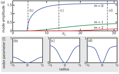
Figure 3: (color online). Details of the bifurcation to circulation. (a) Numerically-evaluated steady state amplitudes $|S_{0}^{(m)}|$ of Bessel series expansion for axisymmetric part of order parameter $S$ at varying activity $\sigma_{0}$, with $d^{(r)}=d^{(s)}=0.025$. (b-d) Profiles of $S$ at indicated points (b-d) in (a).

In order to confirm that the circulating configuration is steady at long times, we must turn to simulations of the fully nonlinear dynamics. In the following numerical studies we vary the dipolar activity $\sigma_{0}$ while fixing the diffusion constants at $d^{(r)}=d^{(s)}=0.025$, and use the eigendecomposition ${\bm{\mathsf{Q}}}=S({\mathbf{n}}{\mathbf{n}}-{\mathbf{{I}}}/2)$, where the order parameter $S$ and (headless) director ${\mathbf{n}}$ are the degree of local alignment and the average alignment direction, respectively. For sufficiently weak activity above $\sigma^{*}$, a stable steady state emerges of circulation about the system center (Fig. 2a&d). The spiral pattern of the nematic director field is reminiscent of the predictions of Kruse et al. Kruse2004 for polar systems (see also Marenduzzo2010, ; Elgeti2011, ). Higher mode contributions can be examined by expanding the order parameter as $S(r,\theta)=\sum_{n}S_{n}(r)e^{in\theta}$, and applying an appropriate $n=0$ mode expansion $S_{0}(r)=\sum_{m=0}^{\infty}S_{0}^{(m)}J_{2}(2y_{m}r)$ where $J_{2}^{\prime}(y_{m})=0$ and $y_{m}<y_{m+1}$. Mode amplitudes are extracted using orthogonality of the radial basis. Figure 3 shows the steady-state values of the first three amplitudes $|S_{0}^{(m)}|$ as functions of $\sigma_{0}$.

At larger values of $\sigma_{0}$, the steady state exhibits defect separation: the central axisymmetric spiral defect in the nematic director field (with topological charge $+1$) splits into two closely spaced hyperbolic defects (each of charge $+1/2$), illustrated in Fig. 2b&e. The system still possesses fluid circulation about the central axis, due to the symmetric positioning of the defects. Defect separation is perhaps unsurprising if we make contact with liquid crystal theory; for approximately isolated defects, the free energy penalty per defect is proportional to the square of its topological charge LubenskyProst1992 , rendering two $+1/2$ defects favorable over a single $+1$ spiral. Indeed, de las Heras et al. delasHeras2009 recently investigated the equivalent confined setup for a microscopic two-dimensional liquid crystal and always encountered defect separation.

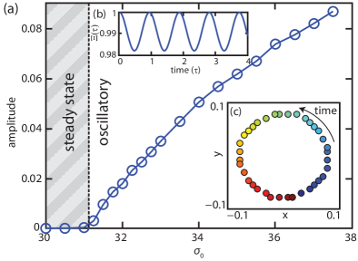
Figure 4: (color online). Secondary bifurcation to oscillatory dynamics. (a) Amplitude of oscillation of the velocity correlation function $\Xi(\tau)$ vs. $\sigma_{0}$, with $d^{(r)}=d^{(s)}=0.025$, showing a bifurcation from steady defect separation to oscillatory behavior at a critical value of $\sigma_{0}$. (b) $\Xi(\tau)$ for $\sigma_{0}=32$ showing periodic oscillatory behavior. (c) Position of flow circulation center over time for $\sigma_{0}=32.75$ during one oscillation period.

As $\sigma_{0}$ is increased beyond a new critical value, the steady state is unstable and the system bifurcates into a regime of periodic oscillation, where the time symmetry is broken. The $+1/2$ defect pair (Fig. 2c) execute periodic ‘orbits’ around each other, with the flow circulation center offset from the origin (Fig. 2f), following a quasi-circular trajectory (Fig. 4c). These states can be analyzed by examining the correlation function Schaller2010

$$\Xi(\tau)\equiv\left\langle\frac{\langle{\mathbf{v}}({\mathbf{x}},t)\cdot{\mathbf{v}}({\mathbf{x}},t-\tau)\rangle_{\mathbf{x}}}{\langle{\mathbf{v}}({\mathbf{x}},t)\cdot{\mathbf{v}}({\mathbf{x}},t)\rangle_{\mathbf{x}}}\right\rangle_{t}$$

where the temporal average is taken over late times when the oscillatory state is fully established. Extracting the amplitude $A$ of oscillation of $\Xi$ (Fig. 4b) we numerically determine a bifurcation diagram as a function of $\sigma_{0}$ as in Fig. 4a. There is a clear threshold for the onset of periodic oscillations. A similar oscillatory bifurcation has been observed by Giomi et al. Giomi for a dense active nematic in a channel geometry, suggesting that such behavior may be a fundamental property of active nematics, though the exact form taken will be heavily dependent on geometry and topology. Were this system an annulus, rather than a disc, behavior more closely resembling the ‘back and forth’ oscillations of Giomi could be conjectured as a regime beyond the spontaneous flow of Furthauer2012 .

Motivated by principles of cytoplasmic streaming, we have constructed a clean, simple model for a dilute suspension of extensile force-generating filaments in total geometric confinement, and have demonstrated that inclusion of elementary hydrodynamics is entirely sufficient to yield spontaneous self-organization, in spite of the absence of more complex local interaction terms. In an experimental realization, the prediction of a critical activity for transition from quiescence to circulation can be tested by varying the viscosity or motor activity, perhaps through temperature or ATP concentration. Modern realizations of the Yotsuyanagi’s experiment could provide a wealth of information on this type of bifurcation.

- (1) J. Verchot-Lubicz and R.E. Goldstein, Protoplasma 240, 99 (2009).
- (2) R.E. Goldstein, I. Tuval and J.W. van de Meent, Proc. Natl. Acad. Sci. USA 105, 3663 (2008).
- (3) Y. Yotsuyanagi, Cytologia 18, 146 (1953); 18, 202 (1953).
- (4) N. Kamiya, Protoplasmic Streaming (Springer-Verlag, Berlin, 1959).
- (5) R. Jarosch, Protoplasma 47, 478 (1956).
- (6) T. Vicsek, A. Czirók, E. Ben-Jacob, I. Cohen and O. Shochet, Phys. Rev. Lett. 75, 1226 (1995); J. Toner and Y. Tu, Phys. Rev. E 58, 4828 (1998); J. Toner, Y. Tu and S. Ramaswamy, Ann. Phys. 318, 170 (2005).
- (7) R. A. Simha and S. Ramaswamy, Phys. Rev. Lett. 89, 058101 (2002).
- (8) R. Voituriez, J.F. Joanny, and J. Prost, Europhys. Lett. 70, 404 (2005).
- (9) K. Kruse, J.F. Joanny, F. Jülicher, J. Prost, and K. Sekimoto, Phys. Rev. Lett. 92, 078101 (2004).
- (10) J. Elgeti, M.E. Cates and D. Marenduzzo, Soft Matter 7, 3177 (2011).
- (11) K. Kruse, J.F. Joanny, F. Jülicher, J. Prost and K. Sekimoto, Eur. Phys. J. E 16, 5 (2005).
- (12) L. Giomi and M.C. Marchetti, Soft Matter 8, 129 (2011).
- (13) L. Giomi, L. Mahadevan, B. Chakraborty and M.F. Hagan, Phys. Rev. Lett. 106, 218101 (2011); Nonlinearity 25, 2245 (2012).
- (14) G. Salbreux, J. Prost and J.F. Joanny, Phys. Rev. Lett. 103, 058102 (2009).
- (15) V. Schaller, C.Weber, C. Semmrich, E. Frey, and A.R. Bausch, Nature 467, 73 (2010).
- (16) S. Fürthauer, M. Neef, S.W. Grill, K. Kruse and F. Jülicher, New J. Phys. 14 023001 (2012).
- (17) D. Saintillan and M.J. Shelley, Phys. Fluids 20, 123304 (2008); Phys. Rev. Lett. 100, 178103 (2008).
- (18) C. Helzel and F. Otto, J. Comput. Phys. 216, 52 (2006).
- (19) A.A. Pahlavan and D. Saintillan, Phys. Fluids 23, 011901 (2011).
- (20) M. Doi and S.F. Edwards, The Theory of Polymer Dynamics (Oxford University Press, USA,1988).
- (21) P.G. de Gennes and J. Prost, The Physics of Liquid Crystals (Clarendon Press, Oxford, 1995).
- (22) A. Baskaran and M.C. Marchetti, Phys. Rev. E 77, 011920 (2008).
- (23) F.G. Woodhouse and R.E. Goldstein, in preparation.
- (24) E.J. Hinch and L.G. Leal, J. Fluid Mech. 76, 187 (1976).
- (25) D. Marenduzzo and E. Orlandini, Soft Matter 6, 774 (2010).
- (26) T. Lubensky and J. Prost, J. Phys. II 2, 371 (1992).
- (27) D. de las Heras, E. Velasco and L. Mederos, Phys. Rev. E 79, 061703 (2009).