Gutzwiller Magnetic Phase Diagram of the Undoped $t-t^{\prime}-U$ Hubbard Model

Abstract

We calculate the magnetic phase diagram of the half-filled $t-t^{\prime}-U$ Hubbard model as a function of $t^{\prime}$ and $U$, within the Gutzwiller approximation RPA (GA+RPA). As $U$ increases, the system first crosses over to one of a wide variety of incommensurate phases, whose origin is clarified in terms of double nesting. We evaluate the stability regime of the incommensurate phases by allowing for symmetry-breaking with regard to the formation of spin spirals, and find a crossover to commensurate phases as $U$ increases and a full gap opens. The results are compared with a variety of other recent calculations, and in general good agreement is found. For parameters appropriate to the cuprates, double occupancy should be only mildly suppressed in the absence of magnetic order, inconsistent with a strong coupling scenario.

I Introduction

An important issue in the Hubbard model is the nature of the metal-insulator transition, whether it is more Mott-like (driven by suppression of double occupancy, with no accompanying magnetic order) or more Slater-like (associated with magnetic order and a Stoner-factor instability). The question is rather subtle, since for instance a Mott phase can have a significant exchange coupling, which can lead to a parasitic magnetic order at low temperatures. Alternatively, critical fluctuations in a two-dimensional system will drive the magnetic ordering temperature to zero (Mermin-Wagner theorem) while leaving behind a finite temperature pseudogap. Recently Tocchio, Becca, Parola, and Sorella (TBPS)TBPS ; BTS carried out a variational calculation of the $t-t^{\prime}-U$ Hubbard model at half filling, and found that the whole $T=0$ phase diagram, Fig. 1(a) is dominated either by paramagnetic phases or by phases with long-range magnetic order (solid green line), except for a small window of nonmagnetic insulator (‘spin liquid’ – dashed green line). Here we show that the ordered magnetic phase boundaries can be well reproduced by simpler Gutzwiller calculations, and that all of these instabilities are only weakly renormalized from the RPA values. These calculations are sufficiently simple that full allowance can be made for incommensurability [TBPS only studied antiferromagnetic order at $(\pi,\pi)$ and $(\pi,0)$], leading to a much richer phase diagram. The domain where TBPS found the spin liquid phase is characterized by a large number of competing phases, leading to potential frustration.

Using a Gutzwiller approximation (GA), Brinkman and Rice (BR)BR found a sharp metal-insulator transition at a critical $U=U_{BR}$, where the effective mass diverges and the average double occupancy $n_{d}$ goes continuously to zero. The BR line is $U_{BR}=8|E_{k}|$, where $E_{k}$ is the average kinetic energy per carrier below the Fermi energy $E_{F}$. While the sharp second order transition is now known to be an artifact of the simplified variational schemeFaz , $U_{BR}$ signals a crossover to a regime of small $n_{d}$, and hence can still serve as a measure of strong correlations.

However, we will show in the present paper that the BR transition usually takes place at much larger $U$ than a magnetic instability towards an incommensurate magnetic state. We will give a detailed analyis of these instabilites in terms of double nesting and discuss the differences between Hartree-Fock (HF) and the GA approach concerning the magnetic phase diagram. Before presenting the corresponding results in Sec. III we briefly introduce the model and formalism in Sec. II and conclude our discussion in Sec. IV.

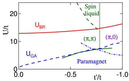
Figure 1: (Color online.) Phase diagram, as a function of $U$ and $t^{\prime}$, showing $U_{BR}$ (red solid line), and calculations from Ref. TBPS (green lines). Shown also are GA+RPA calculations $\tilde{U}_{GA}$ in which the momentum of the instability is restricted to be $(\pi,\pi)$ [dashed blue lines] or $(\pi,0)$ [dot-dashed blue lines].

II Model and Formalism

Starting point is the two-dimensional one-band Hubbard model

$$H=\sum_{i,j,\sigma}t_{ij}c_{i,\sigma}^{\dagger}c_{j,\sigma}+U\sum_{i}n_{i,\uparrow}n_{i,\downarrow},$$ (1)

where $c_{i,\sigma}$ ($c^{\dagger}_{i,\sigma}$) destroys (creates) an electron with spin $\sigma$ at site $i$, and $n_{i,\sigma}=c_{i,\sigma}^{\dagger}c_{i,\sigma}$. $U$ is the on-site Hubbard repulsion and $t_{ij}$ denotes the hopping parameter between sites $i$ and $j$. In the present paper we restrict to hopping between nearest ($\sim t$) and next-nearest ($\sim t^{\prime}$)neighbors leading to a dispersion in momentum space $\epsilon^{0}_{\bf k}=-2t[\cos(k_{x})+\cos(k_{y})]-4t^{\prime}\cos(k_{x})\cos(k_{y})$.

Our approach is based on a generalized GA GEBHARD supplemented with Gaussian fluctuations (GA+RPA) goetz01 in order to evaluate the magnetic instabilities. Since in the following we will also calculate spiral states we use a spin-rotational invariant Gutzwiller energy functional as derived e.g. in Ref. jose06,

$$E^{GA}=\sum_{i,j}t_{ij}\langle{\bf\Psi_{i}}^{\dagger}{\bf z_{i}}{\bf z_{j}}{\bf\Psi_{j}}\rangle+U\sum_{i}D_{i}$$ (2)

and $D_{i}$ denote the variational (’double occupancy’) parameters.

We have also defined the spinor operators

$${\bf\Psi_{i}}^{\dagger}=(c_{i\uparrow}^{\dagger},c_{i\downarrow}^{\dagger})\,\,\,\,\,\,{\bf\Psi_{i}}=\left(\begin{array}[]{c}c_{i\uparrow}\\ c_{i\downarrow}\end{array}\right)$$

and the ${\bf z}$-matrix

$${\bf z}_{i}=\left(\begin{array}[]{cc}z_{i\uparrow}\cos^{2}\frac{\varphi_{i}}{2}+z_{i\downarrow}\sin^{2}\frac{\varphi_{i}}{2}&\frac{S_{i}^{-}}{2S_{i}^{z}}[z_{i\uparrow}-z_{i\downarrow}]\cos\varphi_{i}\\ \frac{S_{i}^{+}}{2S_{i}^{z}}[z_{i\uparrow}-z_{i\downarrow}]\cos\varphi_{i}&z_{i\uparrow}\sin^{2}\frac{\varphi_{i}}{2}+z_{i\downarrow}\cos^{2}\frac{\varphi_{i}}{2}\end{array}\right)$$

with

$$\tan^{2}\varphi_{i}=\frac{S_{i}^{+}S_{i}^{-}}{(S_{i}^{z})^{2}}.$$

In the limit of a vanishing rotation angle $\varphi$ the ${\bf z}$-matrix becomes diagonal and the renormalization factors

$$z_{i\sigma}=\frac{\sqrt{(1-\rho_{i}+D_{i})(\frac{1}{2}\rho_{i}+\frac{S_{i}^{z}}{\cos(\varphi_{i})}-D_{i})}+\sqrt{D_{i}(\frac{1}{2}\rho_{i}-\frac{S_{i}^{z}}{\cos(\varphi_{i})}-D_{i})}}{\sqrt{(\frac{1}{2}\rho_{i}+\frac{S_{i}^{z}}{\cos(\varphi_{i})})(1-\frac{1}{2}\rho_{i}-\frac{S_{i}^{z}}{\cos(\varphi_{i})})}}$$

reduce to those of the standard GA ($\equiv z_{0}$ for a paramagnetic system). Spiral solutions are then computed by minimizing $E^{GA}$ with respect to a homogeneous rotation of spins with wave-vecor ${\bf Q}$

$$S_{i}^{x} = S_{0}\cos({\bf QR}_{i})$$ (3)

$$S_{i}^{y} = S_{0}\sin({\bf QR}_{i}).$$ (4)

In order to compute the magnetic instabilites one can derive an equation similar to the Stoner criterion $U_{HF}=1/max\{\chi_{0}(q)\}$ in HF+RPA. Here

$$\chi_{0}(q)=-{1\over N}\sum_{{\bf k},\sigma}{n_{{\bf k}+{\bf q},\sigma}-n_{{\bf k},\sigma}\over\epsilon^{0}_{{\bf k}+{\bf q}}-\epsilon^{0}_{{\bf k}}}$$

denotes the bare static susceptibility, and the maximum is taken over all $q$-values.

In order to derive the corresponding condition within the GA one has to calculate the response of the system to an external perturbation which couples to the spin degrees of freedom. This can be achieved by expanding the energy functional Eq. 2 up to quadratic order in the (spin)density fluctuations sei04 which yields the generalized GA Stoner criterion

$$max\{U_{GA}\chi_{0}(q)\}=1,$$ (5)

with an effective magnetic interaction

$$U_{GA}=\left[N_{q}+M_{q}[2\bar{E}_{1}+M_{q}(\bar{E}_{1}^{2}-\bar{E}_{2}^{2})\chi_{0}/z_{0}^{2}]\right]/z_{0}^{2}.$$ (6)

The parameters $N_{\bf q}$ and $M_{\bf q}=z_{0}(z^{\prime}-z^{\prime}_{+-})$ are defined in the Appendix of Ref.DLGS, and

$$\bar{E}_{i=1,2}=-{1\over N\chi_{0}}\sum_{{\bf k},\sigma}(\epsilon^{0}_{{\bf k}+{\bf q}}+\epsilon^{0}_{{\bf k}})^{i}{n_{{\bf k}+{\bf q},\sigma}-n_{{\bf k},\sigma}\over\epsilon^{0}_{{\bf k}+{\bf q}}-\epsilon^{0}_{{\bf k}}}.$$ (7)

As discussed in Refs. MGu, ; DLGS, the effective magnetic interaction $U_{GA}\leq U$ and saturates as the bare $U\rightarrow\infty$ whereas in HF+RPA, $U$ can be arbitrarily large. As a consequence, for a given momentum ${\bf q}$ HF+RPA yields a magnetic transition at any doping whereas the corresponding instabilities within the GA are usually confined to a specific doping range.

In the next section we compare our results with those of TBPS which are based on a Gutzwiller variational calculation (without making the GA). In their approach magnetic phases are based on HF groundstates while the spin liquid phase is based on a BCS ground state. The calculations go beyond simple Gutzwiller by including a Jastrow factor and a backflow correction.

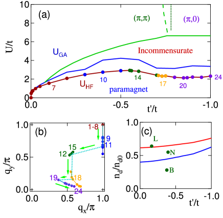
Figure 2: (Color online.) (a) Phase diagram obtained including the regime of incommensurate phases, comparing $U_{HF}$ (brown line) and $U_{GA}$ (blue line). Shown also is the line of first order transitions to commensurate $(\pi,\pi)$ or $(\pi,0)$ order (light green solid line) and the $(\pi,\pi)$ to $(\pi,0)$ crossover line (light green dashed line). For ease in comparisons, the TBPS crossover line (green dotted line) from Fig. 1 is reproduced. To illustrate the dominant $q$-vector (Fig. 2(b)), the HF+RPA points are color coded and numbered consecutively, although only some of the numbers are indicated. (b) Position of the dominant susceptibility peak in HF+RPA, color code and numbers match the values in (a). Note that some extra, metastable points are included, not shown in (a). Blue dotted line traces evolution of stable points. (c) $n_{d}/n_{d0}$ as a function of $t^{\prime}$, assuming a constant $U=8t$ (red line) or $10t$ (blue line). Here $n_{d}$ is the double occupancy, and $n_{d0}=0.25$ is its uncorrelated value. Symbols indicate experimental dispersion renormalization $Z_{disp}$ as a function of $t^{\prime}$, from Ref. Arun3, , which should be an experimental measure of $n_{d}/n_{d0}$. Letters refer to L = La_2-xSr_xCuO₄; N = Nd_2-xCe_xCuO_4±δ; B = Bi₂Sr₂CaCu₂O₈.

III Results

Figure 1 compares the $t^{\prime}/t-U$ phase diagram of TBPSTBPS ; BTS (green lines) with the Brinkman-Rice transition $U_{BR}$ (red solid line) and with the Gutzwiller transition $\tilde{U}_{GA}$, restricted to only $(\pi,\pi)$ [$(\pi,0)$] magnetic order (dashed [dotted] blue line). It is seen that while the spin liquid phase falls above $U_{BR}$, magnetic phases arise for much lower $U$s, and the commensurate GA transitions are in excellent agreement with $U_{TBPS}$. Since the phase boundaries depend only on $|t^{\prime}|$, we illustrate only the situation $t^{\prime}<0$ appropriate to the cuprates.

However, in general competing incommensurate phases become unstable first, due to Fermi surface nesting, Fig. 2(a), which compares the full $U_{GA}$ (blue line) with $U_{HF}$ (brown line). While the HF+RPA calculation overestimates the stability of the magnetic phase, the overestimate is not very large.foot1 Moreover, in all cases the most unstable $q$ vector (along these symmetry lines) is the same for the HF+RPA and the GA+RPA calculations. Thus the main effect of the GA is to renormalize $U\rightarrow U_{GA}<U$, thereby reducing the range of the magnetic ordered phases. In Fig. 2(a) the HF+RPA calculations are coded with variously colored circles which match the points in Fig. 2(b), denoting the ordering $q$-vectors. These changes are associated with the evolution of the Fermi surface (FS) with $t^{\prime}$, as discussed below.

Since the experimental $U$’s in cuprates fall in the range $\sim 6-8t$, Fig. 1 suggests the cuprates are closer to Slater than to Mott physics. Within the BR model, the double occupancy at half filling is given by $n_{d}/n_{d0}=1-(U/U_{BR})^{2}=m/m^{*}$, where $n_{d0}=0.25$ is the uncorrelated double occupancy and $m^{*}$ the renormalized mass. In Fig. 2(c) estimates for the double occupancy $n_{d}$ are plotted within the GA, for an assumed $U=8t$, $10t$, representative of the cuprates. The relatively small reduction of $n_{d}$ explains why the HF+RPA results are so accurate. Since $n_{d}\sim 1/m^{*}$, the present results are consistent with the small observed enhancement of the effective mass (circles in Fig. 2(c))Arun3 ; foot2 . Thus, in cuprates the double occupancy $n_{d}$ is reduced not by Mott physics but by strong AFM fluctuations. In fact, the mean-field AFM suppresses double occupancy so well that Gutzwiller projection on an AFM ground state actually increases double occupancy.Faz

In Fig. 2, it must be kept in mind that $U_{HF}$ and $U_{GA}$ define the onset of the magnetic instability, via a Stoner criterion. As $U$ increases beyond the onset, a finite gap is opened and the optimal $q$ can change. At large $U$ the entire Fermi surface is gapped, and the $q$’s which produce the largest gaps are favored.

In order to access this crossover to commensurate phases we compute the energies of spiral textures within the spin rotational invariant extension of the GA fres92 ; sei04 as outlined in Sec. II. The most stable spiral is determined by searching for the spiral wave-vector ${\bf Q}_{min}$ which minimizes the GA energy. For values slightly larger than $U_{GA}$ we consistently find the minimum of the energy landscape $E_{min}({\bf Q}_{min})$ close to the momenta of the instabilities as shown in Fig. 2a. Upon further increasing $U/t$ and depending on $t^{\prime}/t$ the momenta ${\bf Q}_{min}$ shift either towards the diagonal $(0,0)\to(\pi,\pi)$ or towards the line $(\pi,0)\to(\pi,\pi)$. For a critical $U/t$ one then finally finds a first order transition towards either Néel order ${\bf Q}=(\pi,\pi)$ or towards linear antiferromagnetic (LAF) order at ${\bf Q}=(\pi,0)$ [or equivalently ${\bf Q}=(0,\pi)$].WhiSc This first order transition involves a topological transition of the Fermi surface, from a spiral phase with pockets to a fully gapped commensurate phase.

In Fig. 2a we show the first order line (light green) as an upper boundary for the incommensurate regime together with $U_{GA}$ as the lower transition (blue line) between incommensurate spin spirals and paramagnet. The boundary between Néel and LAF order (light green dashed line) is close to the corresponding transition found by TBPSTBPS ; BTS (green dotted line). Note that the (charge-rotationally invariant) GA samples all possible incommensuabilities, so we confirm that the two ordered phases found by TBPS are indeed the only allowed ordered phases for large enough $U$. However, within the present scheme there is no energy gain for projected BCS wave-functions in the repulsive Hubbard model. Therefore, while our simplified scheme allows for a detailed determination of magnetic phase boundaries we cannot access the spin liquid regime found by TBPS (cf. 2c). We also would like to point out that besides spiral textures the incommensurate regime may also contain spin density wave solutions with an associated small charge density modulation. However, for selected solutions we have checked that this has only a marginal influence on the first order transition line which in Fig. 2 is of the order of the line width.

Figures 3 and 4 show how the FS evolves with $t^{\prime}$, and how this is reflected in the peak susceptibility. Fig. 3(a) displays a map of $\chi_{0}({\bf q})$ for $t^{\prime}=-0.55t$, showing that $\chi_{0}$ is dominated by a complex series of ridges, partly defining a diamond-shaped plateau centered at $(\pi,\pi)$. The origin of these structures is readily apparent from Fig. 3(b) using the concept of nesting curves. For the generic case of two Fermi surface segments, a nesting curve can be defined as the locus of all points ${\bf q}={\bf k_{F1}}-{\bf k_{F2}}$, where ${\bf k_{Fi}}$ is a point on the $i$th FS, FS_i, with the restriction that when FS₁ is shifted by ${\bf q}$ it is tangent to FS₂. For the parameters of Fig. 2(a,b) one has one Fermi surface and the nesting curve is simply given by ${\bf q}=2{\bf k}_{F}$ where ${\bf k}_{F}$ is the (anisotropic) Fermi wave vector. The case of two Fermi surfaces is discussed below. The dashed lines are extensions of the nesting curves folded back into the first BZ. It can be seen that all of the sharp structure in $\chi_{0}$ falls along this nesting curve, and the susceptibility peaks correspond to points where two branches of the curve cross. These values indicate $q$-vectors which nest the FS, and the crossing points correspond to double nesting, along two separate regions of the FS (see Fig. 4, below).

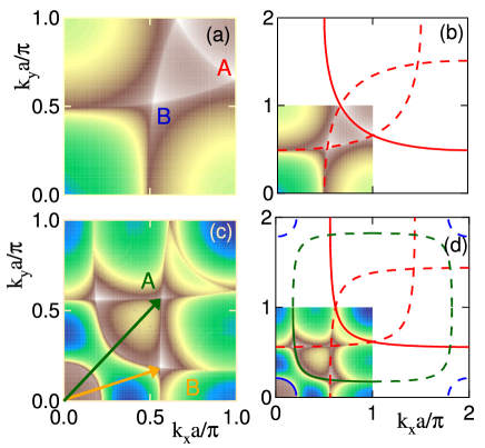
Figure 3: (Color online.) (a) Plot of bare susceptibility $\chi_{0}$ in the first Brillouin zone, for $t^{\prime}=-0.55$, at half filling. (b) Similar plot with nesting curve (solid line) and its folded replicas (dashed lines). (c,d) Similar plots for $t^{\prime}=-0.73$, with additional susceptibility peaks and nesting curves, as discussed in text.

Figures 3(a,b) illustrate the typical behavior at small $|t^{\prime}|$ (appropriate for cuprates). From Fig. 2(a), the peak susceptibility is seen to be approximately commensurate at $(\pi,\pi)$ for $|t^{\prime}|\leq 0.23t$ [brown circles], then becomes vertically incommensurate $(\pi-\delta,\pi)$ for $0.23<|t^{\prime}/t|\leq 0.55$ [blue circles]. For $0.55<|t^{\prime}/t|\leq 0.72$, a diagonal incommensurate $(\pi-\delta,\pi-\delta)$ phase arises [green circles]. Competition between these two phases, corresponding to the points $A$ and $B$ in Fig. 3(a), is also found in hole-doped cupratesMGu . The positions of $A$ and $B$ are readily determined, Fig. 3(b). Peak $A$ lies along the zone boundary ($q_{x}a=\pi$) with

$$q_{y}a=2arccos[{2t-E_{F}\over 2(t-2t^{\prime})}],$$ (8)

while peak $B$ follows the zone diagonal ($q_{x}=q_{y}$) with

$$q_{x}a=2arccos\Bigl{[}\sqrt{E_{F}\over 4t^{\prime}}\Bigr{]}.$$ (9)

The only exception to this rule is the extended nearly-commensurate region near $(\pi,\pi)$ for small $|t^{\prime}|$.

The topology of the band dispersion undergoes a drastic change at $|t^{\prime}|=0.5t$. At that ratio the Van Hove singularity (VHS) moves down to the bottom of the band, leading to a dispersionless band along the $x$ and $y$ axes. Beyond $|t^{\prime}/t|=0.5$, the VHS moves away from the band bottom, but now the point $\Gamma$ changes from the band minimum to a local maximum, opening the possibility of a second FS section. At $|t^{\prime}|=0.71t$, this section crosses the Fermi level at half filling, leading to a more complicated susceptibility map, Fig. 3(c,d), with a second ${\bf q}=2{\bf k}_{F2}$ nesting curve (blue line) centered on $\Gamma$, as well as a ${\bf q}={\bf k}_{F2}-{\bf k}_{F1}$ nesting curve (green line). In all cases the nesting curves match the positions of sharp structure in $\chi_{0}$. [For the inter-FS nesting, the $q$-value corresponds to shifting one FS until it is tangent to the second.] This leads to a greatly increased number of nesting curve intersections, and the $\chi_{0}$ peak shifts, first, briefly, to a $k_{F1}$-mixed nesting curve intersection (orange line in Fig. 2(b)), then to a $k_{F2}$-mixed nesting curve (violet line). Figure 3 provides an example of double nesting, showing two competing $q$-peaks, corresponding to $A$ and $B$ in Fig. 3(c). Here nesting vector A [green arrows] involves double nesting of the large FS [green FSs], while in B [orange arrows] one nesting involves the large FS [brown FS], but the other involves nesting between the large FS and the $\Gamma$-centered pocket [orange FS].

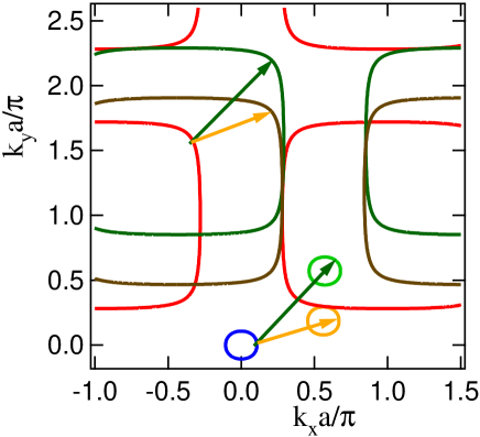
Figure 4: (Color online.) Fermi surfaces (red and blue lines) and the $q$-shifted versions, illustrating two (competing) examples of double nesting. Data are for $t^{\prime}=-0.73t$, $x=0$, as in Fig. 2 (c,d) [arrows].

IV Conclusions

Increasingly, it is becoming clear that many of the complications of strongly correlated systems have to do with competing phases, whether leading to nanoscale phase separation, ‘stripes’, or frustration. However, part of the problem is a very incomplete understanding of phase competition even at weak coupling, and how the competing phases evolve between weak and strong coupling. In this sense the magnetic instability of the two-dimensional Hubbard model provides an ideal case study, having a parameter space which is two-dimensional ($q_{x}$, $q_{y}$). In HF+RPA $U$ is constant and the competition reduces to finding the maximum of $\chi_{0}$ (Stoner criterion). We find that the Gutzwiller correction leads only to quantitative (close to numerical results) and not qualitative (gain/loss of new phase) changes. Hence, the nesting curves introduced herein should provide valuable tools for determining the optimal nesting vectors for many different correlated materials, and how these evolve with doping, temperature, impurity scattering, etc.

In commenting on the calculation of TBPS, Becca, Tocchio, and SorellaBTS summarized earlier attempts to characterize the phase diagram of the model: “Remarkably, all these numerical approaches give very different results for the ground-state properties of this simple correlated model. In fact, there are huge discrepancies for determining the boundaries of various phases, but also for characterizing the most interesting non-magnetic insulator.” Here, we have presented two additional phase diagrams, in HF and GA+RPA approximations. A key point is that with increasing U the first instability is generically to an incommensurate phase controlled by Fermi surface nesting. For larger $U$ the FS is fully gapped, nesting is unimportant, and the only stable magnetic phases are the two commensurate phases found by TBPS. For the rest our phase boundaries agree with TBPS except for the spin liquid phase which is beyond the capabilities of a simple mean field approximation.

- (1) L.F. Tocchio, F. Becca, A. Parola, and S. Sorella, Phys. Rev. B78, 041101(R) (2008).
- (2) F. Becca, L.F. Tocchio, and S. Sorella, Proc. HFM2008 Conf., arXiv:0810.0665.
- (3) W.F. Brinkman and T.M. Rice, Phys. Rev. B2, 4302 (1970).
- (4) P. Fazekas, “Lecture Notes on Electron Correlation and Magnetism,” (World Scientific, Singapore, 1999).
- (5) F. Gebhard, Phys. Rev. B 41, 9452 (1990).
- (6) G. Seibold and J. Lorenzana, Phys. Rev. Lett. 86, 2605 (2001).
- (7) J. Lorenzana and G. Seibold, Low Temp. Physics 32, 320 (2006).
- (8) G. Seibold, F. Becca, P. Rubin, and J. Lorenzana, Phys. Rev. B 69, 155113 (2004).
- (9) C. Kusko and R.S. Markiewicz, Phys. Rev. B65, 041102(R) (2001).
- (10) R.S. Markiewicz, J. Lorenzana, G. Seibold, and A. Bansil, unpublished.
- (11) A. Di Ciolo, J. Lorenzana, M. Grilli, and G. Seibold, Phys. Rev. B79, 085101 (2009).
- (12) G. Kotliar and A.E. Ruckenstein, Phys. Rev. Lett. 57, 1362 (1986).
- (13) Part of this difference is due to the fact that the RPA calculation samples all values (Fig. 2(a), while the Gutzwiller calculation was restricted to the high symmetry axes, .
- (14) R.S. Markiewicz, S. Sahrakorpi, M. Lindroos, Hsin Lin, and A. Bansil, Phys. Rev. B72, 054519 (2005). In Fig. 2(c) we introduce an effective , which controls the energy of the Van Hove singularity.
- (15) While is determined at finite doping, for [] is not expected to vary greatly with dopingFaz .
- (16) R. Frésard and P. Wölfle, J. Phys. Condens. Matter 4, 3625 (1992).
- (17) S. Sahrakorpi, R. S. Markiewicz, Hsin Lin, M. Lindroos, X. J. Zhou, T. Yoshida, W. L. Yang, T. Kakeshita, H. Eisaki, S. Uchida, Seiki Komiya, Yoichi Ando, F. Zhou, Z. X. Zhao, T. Sasagawa, A. Fujimori, Z. Hussain, Z.-X. Shen, and A. Bansil, Phys. Rev. B78, 104513 (2008).