Abstract

Chaos transition, as an important topic, has become an active research subject in non-linear science. By considering a Dicke Hamiltonian coupled to a bath of harmonic oscillator, we have been able to introduce a logistic map with quantum corrections. Some basic dynamical properties, such as Lyapunov exponents and bifurcation diagram of the model are studied. we show that in this model, the transition from integrable motion to periodic, chaotic and hyperchaotic as the control parameter $r$ is increased.

PACS number(s): 05.45.+b, 87.23.Cc

1 Introduction

Investigation in the area of quantum dots couple with another quantum dot or one external field has received a great deal of attention in recent years. Deterministic equations have been used nowadays in many applications [1] . For instance, a chaotic system is one which displays complex and unpredictable behavior. These systems with some of properties such as sensitivity to initial condition [2], system parameter, ergodicity [3] and mixing [4]. One of the popular fields of quantum chaos addresses quantum maps. Classical maps exhibit the properties of chaotic dynamical systems. Various chaotic maps use in Cryptography, Watermarking, Random number generators and lots of other fields. On the other hand, a big number of researches have been dedicated so far to quantum maps as paradigms of quantum chaos [5, 6]. M.Goggin et al. in their work, the quantum correction were made by introducing a periodic noise to a model of oscillatory system coupled to a bath of oscillators. They derive a new logistic map with quantum computing that illustrate a period-doubling route to chaos [7]. The quantization schemes for maps are different and many classically chaotic maps have been quantized including the standard map [8, 9], logistic map [7], baker map on the torus [10, 11, 12] and on sphere [13]. In present paper we introduce generalized Dick model has been considered to present a new quantum map which demonstrates positive lyapunov exponents.The comparison between analytically studied and simulation results indicate that the propose methods provide good estimates. The paper is organized as follows. In section 2, introduces the model. In section 3, we calculate the lyapunov exponents and KS-entropy. Finally, in section 4, we conclude the paper. Respective appendix can be found at the end of paper.

2 The model

We start with the hamiltonian:

$$H=a^{{\dagger}}a+\omega_{A}J_{z}+\frac{\gamma}{\sqrt{N}}(a^{{\dagger}}+a)(J_{-}+J_{+})+\frac{\gamma}{\sqrt{N}}V(J_{-},J_{+})\Sigma_{n}\delta(t-nT),$$ (1)

this hamiltonian is the generalized Dick Hamiltonian. In fact we add a delta function to Dick Hamiltonian. Therefore, $a$ and $a^{{\dagger}}$ bosonic annihilation and creation operators, energy separation of N two-level atoms equal to $\hbar$${\tilde{\omega}}_{A}$ , $\hbar=1$ , field of frequency ${\tilde{\omega}}_{f}$, ${\omega}_{A}={\tilde{\omega}}_{A}/{\tilde{\omega}}_{f}\geq 0$ is given in units of the frequency of the field, ${\gamma}={\tilde{\gamma}}/{\tilde{\omega}}_{f}$ is the coupling parameter. ${J}_{z}$ the atomic relative population operator, and ${J}_{\pm}$ the atomic transition operators. The commutation relations for the fermionic operator J are:

$[{J_{+},J_{-}}]=2J_{z}$ , $[J_{z},J_{\pm}]=\pm J_{\pm}$ , $[a,a^{{\dagger}}]=1$.

Heisenberg equation of motion reads:

$$\dot{J_{+}}=i[H,J_{+}],$$ (2)

by considering $(-i\frac{\gamma}{\sqrt{N}}[J_{+},V(J_{+},J_{-})]=f(J_{-},J_{+}))$,
we have :

$$\left\{\begin{array}[]{l}$$\dot{J_{+}}=i\omega_{A}J_{z}-i\frac{\gamma}{\sqrt{N}}(a^{{\dagger}}+a)(2J_{z})+f(J_{+},J_{-})\Sigma_{n}\delta(t-nT),\;\;\;\;\;\;\;(A1)$$\\ \\ \dot{a}=-ia-i\frac{\gamma}{\sqrt{N}}(J_{-}+J_{+}).\;\;\;\;\;\;\;\;\;\;\;\;\;\;\;\;\;\;\;\;\;\;\;\;\;\;\;\;\;\;\;\;\;\;\;\;\;\;\;\;\;\;\;\;\;\;\;\;\;\;\;\;\;\;\;\;(A2)\end{array}\right.$$

In order to obtain an equation for ${J_{+}}(t)$, we substitute the solution of (A2) into (A1):

$$\dot{J_{+}}=i\omega_{A}J_{+}-i\frac{\gamma}{\sqrt{N}}a^{{\dagger}}(0)(\exp(it))(2J_{z})-i\frac{\gamma}{\sqrt{N}}a(0)(\exp(-it))(2J_{z})$$

$$+f(J_{+},J_{-})\Sigma_{n}\delta(t-nT),$$ (3)

we integrate of Eq. (3) from t= nT to t= (n+1)T, so as to obtain

$$J_{+}((n+1)T)-J_{+}(nT)\exp(i\omega_{A}T)=\left[-i\frac{\gamma}{\sqrt{N}}a^{{\dagger}}(0){\int_{nT}}^{(n+1)T}(2J_{z})\exp(i(1-\omega_{A})t)dt\right.$$

$$\left.-i\frac{\gamma}{\sqrt{N}}a(0){\int_{nT}}^{(n+1)T}(2J_{z})\exp(-i(1+\omega_{A})t)dt\right]+f(J_{+}(nT),J_{-}(nT))\exp(i\omega_{A}T).$$ (4)

We assume that $<a(0)>=0$ , $<a^{{\dagger}}(0)>=0$, the expectation value of $J_{+}$ can be expressed in:

$$<J_{+}((n+1)T)>=\left(<J_{+}(nT)>+<f(J_{+}(nT),J_{-}(nT))>\right)\exp(i\omega_{A}T).$$ (5)

For comparison our quantum results to the familiar logistic map we choose the “force”:

$$f(J_{+(n)},J_{-(n)})=-J_{+(n)}+r\left(J_{+(n)}-J_{-(n)}J_{+(n)}\right)\exp(-i\omega_{A}T),$$ (6)

where r is an adjustable parameter. Eq. (5) then becomes :

$$<J_{+(n+1)}>=r\left(<J_{+(n)}>-<J_{-(n)}J_{+(n)}>\right),$$ (7)

where $x=<J_{+}>=<J_{-}>$ , then:

$$x_{n+1}=r(x_{n}-{x_{n}}^{2}).$$

Which is the classical logistic map .

The logistic map is one of the most studied discrete chaotic maps. It was first proposed as pseudo random number generator by Von Neumann in 1947 partly because it had a known algebraic distribution and mentioned later, in 1969, by Knuth[14, 15]. The logistic map is given by:

$$x_{n+1}=rx_{n}(1-x_{n})$$ (8)

where $x_{n}\in(0,1)$ and $r$ are the system variable and parameter, respectively, and $n$ is the number of iterations. Thus, given an initial value $x_{0}$ and a parameter $r$. In this paper, we refer to $x_{0}$ and $r$ as the initial state of the logistic map.

$$x_{n+1}=rx_{n}(1-x_{n}),\;\;\;\;\;for\;\;\;\;\ x_{n}\in(0,1),\;\;\;and\;\;\;r\in(3.99996,4]$$

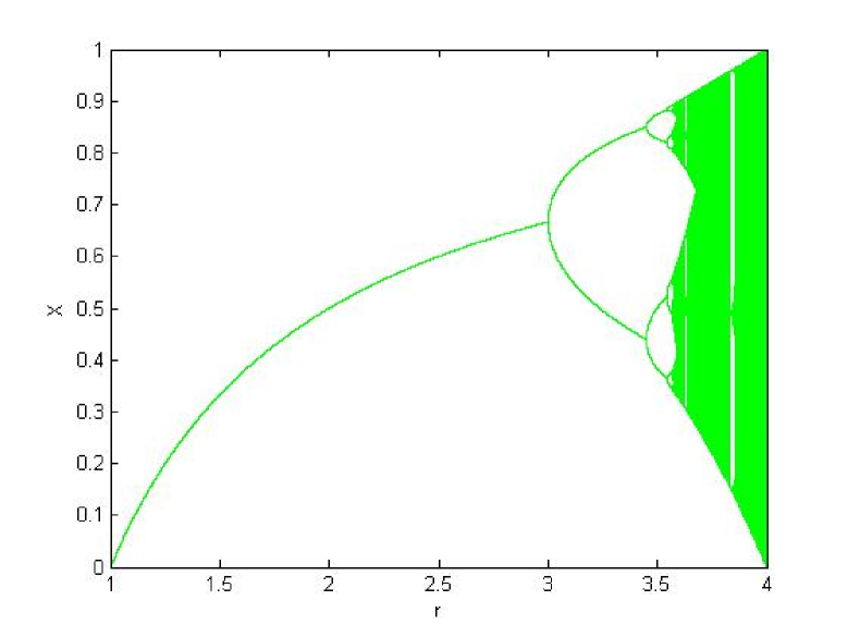
Figure 1: Bifurcation diagram for the logistic map, $x_{n+1}=rx_{n}(1-x_{n})$ when the parameter $r$ is varied from 1 to 4.

and its behavior is full chaotic(Fig 1). The choice of $r$ in the equation above guarantees the existence of a chaotic orbit that can be shadowed by only one map as stated in [16]. The lyapunov exponent h is taken as a measure of the “chaoticness” of N quantum dots coupled with a single bosonic mode. The dynamical systems, even the discrete-time and one-variable ones have different types of behaviour. The system can be in a fixed point and nothing changes, the trajectory of the system may also be a cycle with a certain period. Fixed point and periodic orbits may be stable or unstable. We are usually interested in an invariant measure , i.e. a probability measure that does not change under the dynamics. The probability measure $\rho(x)=\frac{1}{\pi\sqrt{x(1-x)}}$ on [0; 1] is a Sinai-Rulle-Bowen (SRB) measure which is an invariant measure which describes statistically the stationary states of the system and absolutely continues with respect to Lebesgue measure. Entropy sometimes is called uncertainty and sometimes information . In order to study the stability, entropy can be used as an acceptable parameter. Also, by considering SRB measure, it is possible to continue this study with KS-entropy, the well-known measure for chaos in dynamical system. This section introduces the KS-entropy for hierarchy of pair-coupled maps with dynamical parameter. We try to calculate Lyapunov exponent as another tool to study the stability.

$$h={\int_{0}}^{1}\ln|F^{{}^{\prime}}(x)|\rho(x)dx=2{\int_{0}}^{1/2}\frac{\ln|r(1-2x)|}{\pi\sqrt{x(1-x)}}dx,$$ (9)

with change of variable $x={\sin}^{2}(\theta)$ , $dx=2\sin(\theta)\cos(\theta)d\theta$, and using Eq. (9) becomes

$$h=2{\int_{0}}^{\pi/4}\frac{\ln|r(1-2{\sin}^{2}(\theta))|}{\pi\sin(\theta)\cos(\theta)}2\sin(\theta)\cos(\theta)d\theta$$

. (10)

KS-entropy, may also can be written as:

$$h=\ln{r}-\ln{2},$$ (11)

for $r=4\rightarrow h=\ln{2}>0$, it is positive.

For appearance the effect of the quantum correlations by using $J_{+}=<J_{+}>+\delta J_{+}$ and $J_{-}=<J_{-}>+\delta J_{-},$ one gets

$$<J_{+(n+1)}>=r\left(<J_{+(n)}>-<J_{-(n)}><J_{+(n)}>\right)-r<\delta J_{-}\delta J_{+}>.$$ (12)

First, the time derivative of$(\delta J_{+}\delta J_{-})$ is

$${\frac{d}{dt}}(\delta J_{+}\delta J_{-})=\delta\dot{J_{+}}\delta J_{-}+\delta J_{+}\delta\dot{J_{-}}.$$ (13)

Inserting these two expressions $J_{+}=<J_{+}>+\delta J_{+}$ and $J_{-}=<J_{-}>+\delta J_{-}$ into Eq. (6) we end up with

$$f(J_{+},J_{-})=-<J_{+}>-\delta J_{+}+\exp(-iw_{A}T)r(<J_{+}>+\delta J_{+}-<J_{-}><J_{+}>-$$

$$\delta J_{-}\delta J_{+}-<J_{-}>\delta J_{+}-\delta J_{-}<J_{+}>).$$ (14)

Inserting $\dot{J_{+}}=\delta\dot{J_{+}}$ and $\dot{J_{-}}=\delta\dot{J_{-}}$ , into Eq. (3) we obtain:

$$\delta\dot{J_{+}}=iw_{A}(<J_{+}>+\delta J_{+})-i\frac{\gamma}{\sqrt{N}}a^{{\dagger}}(0)(\exp(it))[\delta J_{+}\delta J_{-}-\delta J_{-}\delta J_{+}]-i\frac{\gamma}{\sqrt{N}}a(0)$$

$$(\exp(-it))[\delta J_{+}\delta J_{-}-\delta J_{-}\delta J_{+}]+[-<J_{+}>-\delta J_{+}+\exp(-iw_{A}T)r(<J_{+}>+\delta J_{+}$$

$$-<J_{-}><J_{+}>-\delta J_{-}\delta J_{+}-<J_{-}>\delta J_{+}-\delta J_{-}<J_{+}>)]\Sigma_{n}\delta(t-nT).$$ (15)

Due to

$$\delta\dot{J_{-}}=\delta\dot{J_{+}}^{{\dagger}}=-iw_{A}(<J_{-}>+\delta J_{-})+i\frac{\gamma}{\sqrt{N}}a(0)(\exp(-it))[\delta J_{-}\delta J_{+}-\delta J_{+}\delta J_{-}]+i\frac{\gamma}{\sqrt{N}}{a^{{\dagger}}}(0)$$

$$(\exp(it))[\delta J_{-}\delta J_{+}-\delta J_{+}\delta J_{-}]+[-<J_{-}>-\delta J_{-}+\exp(iw_{A}T)r(<J_{-}>+\delta J_{-}-$$

$$<J_{+}><J_{-}>-\delta J_{+}\delta J_{-}-<J_{+}>\delta J_{-}-\delta J_{+}<J_{-}>)]\Sigma_{n}\delta(t-nT),$$ (16)

Finally, inserting Eq. (15) and Eq. (16) into Eq. (13), we end up with

$${\frac{d}{dt}}(\delta J_{+}\delta J_{-})=\left[iw_{A}(<J_{+}>+\delta J_{+})-i\frac{\gamma}{\sqrt{N}}a^{{\dagger}}(0)(\exp(it))[\delta J_{+}\delta J_{-}-\delta J_{-}\delta J_{+}]-i\frac{\gamma}{\sqrt{N}}a(0)\right.$$

$$(\exp(-it))[\delta J_{+}\delta J_{-}-\delta J_{-}\delta J_{+}]+[-<J_{+}>-\delta J_{+}+\exp(-iw_{A}T)r(<J_{+}>+\delta J_{+}-<J_{-}>$$

$$<J_{+}>-\delta J_{-}\delta J_{+}-<J_{-}>\delta J_{+}-\delta J_{-}<J_{+}>)]\left.\Sigma_{n}\delta(t-nT)\right]{\delta J_{-}}+\delta J_{+}\left[-iw_{A}(<J_{-}>+\delta J_{-})\right.$$

$$+i\frac{\gamma}{\sqrt{N}}a(0)(\exp(-it))[\delta J_{-}\delta J_{+}-\delta J_{+}\delta J_{-}]+i\frac{\gamma}{\sqrt{N}}{a^{{\dagger}}}(0)(\exp(it))[\delta J_{-}\delta J_{+}-\delta J_{+}\delta J_{-}]+[-<J_{-}>$$

$$-\delta J_{-}+\exp(iw_{A}T)r(<J_{-}>+\delta J_{-}-<J_{+}><J_{-}>-\delta J_{+}\delta J_{-}-<J_{+}>\delta J_{-}-\delta J_{+}<J_{-}>)]$$

$$\left.\Sigma_{n}\delta(t-nT)\right].$$ (17)

By integrating Eq. (17), from (nT) to ((n+1)T), and take the expectation value, by taking into account $<\delta J_{-}(nT)>=<\delta J_{+}(nT)>=0$ , $<{a^{{\dagger}}}(0)>=<a(0)>=0$ we obtain:

$$<\delta J_{+}((n+1)T)\delta J_{-}((n+1)T)>=-<\delta J_{+}(nT)\delta J_{-}(nT)>+r\exp(-iw_{A}T)<\delta J_{+}(nT)\delta J_{-}(nT)>$$

$$-r\exp(-iw_{A}T)<J_{-}><\delta J_{+}(nT)\delta J_{-}(nT)>-r\exp(-iw_{A}T)<\delta J_{-}(nT)\delta J_{-}(nT)><J_{+}>+r$$

$$\exp(iw_{A}T)<\delta J_{+}(nT)\delta J_{-}(nT)>-r\exp(iw_{A}T)<\delta J_{+}(nT)\delta J_{-}(nT)><J_{+}>-r\exp(iw_{A}T)$$

$$<\delta J_{+}(nT)\delta J_{+}(nT)><J_{-}>.$$ (18)

The calculation of $<\delta J_{+}\delta J_{+}>$ goes as follows:

$${\frac{d}{dt}}(\delta J_{+}\delta J_{+})=\delta\dot{J_{+}}\delta J_{+}+\delta J_{+}\delta\dot{J_{+}}.$$ (19)

appearance the effect of the quantum correlations by using $J_{+}=<J_{+}>+\delta J_{+}$ and $J_{-}=<J_{-}>+\delta J_{-}$ Eq. (6), one gets:

$$f(J_{+},J_{-})=-<J_{+}>-\delta J_{+}+\exp(-iw_{A}T)r(<J_{+}>+\delta J_{+}-<J_{-}><J_{+}>-$$

$$\delta J_{-}\delta J_{+}-<J_{-}>\delta J_{+}-\delta J_{-}<J_{+}>),$$ (20)

Inserting $\dot{J_{+}}=\delta\dot{J_{+}}$ , into Eq. (3) we obtain:

$$\delta\dot{J_{+}}=iw_{A}(<J_{+}>+\delta J_{+})-i\frac{\gamma}{\sqrt{N}}a^{{\dagger}}(0)(\exp(it))[\delta J_{+}\delta J_{-}-\delta J_{-}\delta J_{+}]-i\frac{\gamma}{\sqrt{N}}a(0)$$

$$(\exp(-it))[\delta J_{+}\delta J_{-}-\delta J_{-}\delta J_{+}]+[-<J_{+}>-\delta J_{+}+\exp(-iw_{A}T)r(<J_{+}>+\delta J_{+}$$

$$-<J_{-}><J_{+}>-\delta J_{-}\delta J_{+}-<J_{-}>\delta J_{+}-\delta J_{-}<J_{+}>)]\Sigma_{n}\delta(t-nT),$$ (21)

Finally, inserting Eq. (21) into Eq. (19), we end up with:

$${\frac{d}{dt}}(\delta J_{+}\delta J_{+})=[iw_{A}(<J_{+}>+\delta J_{+})-i\frac{\gamma}{\sqrt{N}}a^{{\dagger}}(0)(\exp(it))[\delta J_{+}\delta J_{-}-\delta J_{-}\delta J_{+}]-i\frac{\gamma}{\sqrt{N}}a(0)$$

$$(\exp(-it))[\delta J_{+}\delta J_{-}-\delta J_{-}\delta J_{+}]+[-<J_{+}>-\delta J_{+}+\exp(-iw_{A}T)r(<J_{+}>+\delta J_{+}-<J_{-}>$$

$$<J_{+}>-\delta J_{-}\delta J_{+}-<J_{-}>\delta J_{+}-\delta J_{-}<J_{+}>)]\Sigma_{n}\delta(t-nT)]\delta J_{+}+\delta J_{+}[iw_{A}(<J_{+}>+$$

$$\delta J_{+})-i\frac{\gamma}{\sqrt{N}}a^{{\dagger}}(0)(\exp(it))[\delta J_{+}\delta J_{-}-\delta J_{-}\delta J_{+}]-i\frac{\gamma}{\sqrt{N}}a(0)$$

$$(\exp(-it))[\delta J_{+}\delta J_{-}-\delta J_{-}\delta J_{+}]+[-<J_{+}>-\delta J_{+}+\exp(-iw_{A}T)r(<J_{+}>+\delta J_{+}-<J_{-}>$$

$$<J_{+}>-\delta J_{-}\delta J_{+}-<J_{-}>\delta J_{+}-\delta J_{-}<J_{+}>)]\Sigma_{n}\delta(t-nT)].$$ (22)

By integrating Eq. (22), from (nT) to ((n+1)T), and take the expectation value, by taking into account $<\delta J_{-}(nT)>=<\delta J_{+}(nT)>=0$ , $<{a^{{\dagger}}}(0)>=<a(0)>=0$ we obtain:

$$<\delta J_{+}((n+1)T)\delta J_{+}((n+1)T)>\exp(-2i\omega_{A}(n+1)T)-<\delta J_{+}(nT)\delta J_{+}(nT)>\exp(-2i\omega_{A}nT)=$$

$$\exp(-2i\omega_{A}nT)(-<\delta J_{+}(nT)\delta J_{+}(nT)>+\exp(-i\omega_{A}T)r(<\delta J_{+}(nT)\delta J_{+}(nT)>-<J_{-}(nT)>$$

$$<\delta J_{+}(nT)\delta J_{+}(nT)>-<J_{+}(nT)><\delta J_{-}(nT)\delta J_{+}(nT)>))+\exp(2i\omega_{A}nT)(-<\delta J_{+}(nT)$$

$$\delta J_{+}(nT)>+\exp(-i\omega_{A}T)r(<\delta J_{+}(nT)\delta J_{+}(nT)>-<J_{-}(nT)><\delta J_{+}(nT)\delta J_{+}(nT)>-$$

$$<\delta J_{+}(nT)\delta J_{-}(nT)><J_{+}(nT)>)).$$ (23)

By taking into account $<\delta J_{+}(nT)\delta J_{-}(nT)>$=$Y_{n}$ , $<\delta J_{+}\delta J_{+}>$=$Z_{n}$ , $<J_{+}(nT)>$=$X_{n}$ and inserting these values into Eqs. (12), (18) and (23), we obtain:

$$\left\{\begin{array}[]{l}$$\par X_{(n+1)}=r(X_{(n)}-{X_{(n)}}^{2})-rY_{(n)}\;\;\;\;\;\;\;\;\;\;\;\;\;\;\;\;\;\;\;\;\;\;\;\;\;\;\;\;\;\;\;\;\;\;\;\;\;\;\;\;\;\;\;\;\;\;\;\;\;\;\;\;\;\;\;\;\;\;\;\;\;\;\;\;\;(B1)\\ \\ Y_{(n+1)}=-Y_{n}+r\exp(-iw_{A}T)([(1-{X_{(n)}}^{*}\\ +\exp(2iw_{A}T)-X_{(n)}\exp(2iw_{A}T))Y_{n}]\par\par-{Z_{n}}^{*}X_{n}-\exp(2iw_{A}T)Z_{n}{X_{n}}{*})\;\;\;\;\;\;\;\;\;\;(B2)\\ \\ Z_{(n+1)}=-Z_{n}\exp(2iw_{A}T)+r\exp(iw_{A}T)(2Z_{n}-2{X_{n}}{*}Z_{n}-X_{n}{Y_{n}}^{*}-Y_{n}X_{n})\;\;(B3).\end{array}\right.$$

These equations give us lowest-order quantum corrections.We consider $\beta=iw_{A}T$.

3 The onset of quantum chaos

The research on the chaos of Eq. (B) can begin with the analysis on the stability of the fixed point. Assume $(x,y,z)$ is the fixed point of Eq. (B), then $(x,y,z)$ is the solution of the equations below:

$$\left\{\begin{array}[]{l}$$\par x=r(x-{x}^{2})-ry\;\;\;\;\;\;\;\;\;\;\;\;\;\;\;\;\;\;\;\;\;\;\;\;\;\;\;\;\;\;\;\;\;\;\;\;\;\;\;\;\;\;\;\;\;\;\;\;\;\;\;\;\;\;\;\;\;\;\;\;\;\;\;\;\;(C1)\\ \\ y=-y+r\exp(-\beta)([(1-x\\ +\exp(2\beta)-x\exp(2\beta))y]\par\par-zx-\exp(2\beta)zx)\;\;\;\;\;\;\;\;\;\;(C2)\\ \\ z=-z\exp(2\beta)+r\exp(\beta)(2z-2xz-xy-yx)\;\;(C3).\end{array}\right.$$

By considering $\exp(\beta)=a$ and solution Eq. (C) we obtain:

$x=0,$
$(r-1)/r,$
$-(-a^{4}*r+2*a^{3}*r^{2}+2*a^{3}-6*a^{2}*r+2*a*r^{2}+2*a-r)/(a^{4}*r-4*a^{3}*r^{2}+6*a^{2}*r-4*a*r^{2}+r),$

$y=0,$
$0,$

$(-a^{8}*r-2*a^{7}*r^{3}+6*a^{7}*r^{2}+2*a^{7}*r+2*a^{7}+4*a^{6}*r^{4}-8*a^{6}*r^{3}-20*a^{6}*r-4*a^{6}-14*a^{5}*r^{3}+42*a^{5}*r^{2}+14*a^{5}*r+14*a^{5}+8*a^{4}*r^{4}-16*a^{4}*r^{3}-54*a^{4}*r-8*a^{4}-14*a^{3}*r^{3}+42*a^{3}*r^{2}+14*a^{3}*r+14*a^{3}+4*a^{2}*r^{4}-8*a^{2}*r^{3}-20*a^{2}*r-4*a^{2}-2*a*r^{3}+6*a*r^{2}+2*a*r+2*a-r)/(a^{8}*r^{2}-8*a^{7}*r^{3}+16*a^{6}*r^{4}+12*a^{6}*r^{2}-56*a^{5}*r^{3}+32*a^{4}*r^{4}+38*a^{4}*r^{2}-56*a^{3}*r^{3}+16*a^{2}*r^{4}+12*a^{2}*r^{2}-8*a*r^{3}+r^{2}),$

$z=0,$
$0,$
$(2*a^{9}*r^{2}+4*a^{8}*r^{4}-8*a^{8}*r^{3}-4*a^{8}*r^{2}-8*a^{8}*r-16*a^{7}*r^{3}+48*a^{7}*r^{2}+16*a^{7}*r+8*a^{7}+12*a^{6}*r^{4}-24*a^{6}*r^{3}+4*a^{6}*r^{2}-88*a^{6}*r-16*a^{6}-32*a^{5}*r^{3}+92*a^{5}*r^{2}+32*a^{5}*r+48*a^{5}+12*a^{4}*r^{4}-24*a^{4}*r^{3}+4*a^{4}*r^{2}-88*a^{4}*r-16*a^{4}-16*a^{3}*r^{3}+48*a^{3}*r^{2}+16*a^{3}*r+8*a^{3}+4*a^{2}*r^{4}-8*a^{2}*r^{3}-4*a^{2}*r^{2}-8*a^{2}*r+2*a*r^{2})/(a^{1}0*r^{2}-8*a^{9}*r^{3}+16*a^{8}*r^{4}+13*a^{8}*r^{2}-64*a^{7}*r^{3}+48*a^{6}*r^{4}+50*a^{6}*r^{2}-112*a^{5}*r^{3}+48*a^{4}*r^{4}+50*a^{4}*r^{2}-64*a^{3}*r^{3}+16*a^{2}*r^{4}+13*a^{2}*r^{2}-8*a*r^{3}+r^{2}).$

In the thermodynamic limit $\beta\rightarrow 0$ or $a=1$, we have following fixed points:

$(x_{0},y_{0},z_{0})=(0,0,0)$
$(x_{1},y_{1},z_{1})=((r-1)/r,0,0)$
$(x_{2},y_{2},z_{2})=(-(r^{2}-3*r+2)/(4*r-3*r^{2}),(2*r^{4}-10*r^{3}+18*r^{2}-14*r+4)/(9*r^{4}-24*r^{3}+16*r^{2}),(r^{4}-6*r^{3}+13*r^{2}-12*r+4)/(9*r^{4}-24*r^{3}+16*r^{2}))$


We substitute $X_{(n+1)}=X$, $X_{n}=x$, $Y_{(n+1)}=Y$, $Y_{n}=y$, $Z_{(n+1)}=Z$ and $Z_{(n+1)}=z$ into Eq. (B) obtain:

$$\left\{\begin{array}[]{l}$$\par X=r(x-{x}^{2})-ry\;\;\;\;\;\;\;\;\;\;\;\;\;\;\;\;\;\;\;\;\;\;\;\;\;\;\;\;\;\;\;\;\;\;\;\;\;\;\;\;\;\;\;\;\;\;\;\;\;\;\;\;\;\;\;\;\;\;\;\;\;\;\;\;\;(D1)\\ \\ Y=-y+r\exp(-\beta)([(1-x\\ +\exp(2\beta)-x\exp(2\beta))y]\par\par-zx-\exp(2\beta)zx)\;\;\;\;\;\;\;\;\;\;(D2)\\ \\ Z=-z\exp(2\beta)+r\exp(\beta)(2z-2xz-xy-yx)\;\;(D3).\end{array}\right.$$

The corresponding bifurcation diagram of state x with respect to $r$ is giving in Fig. 2.

In order to calculate the lyapunov exponents at $x=x_{0}$, $y=y_{0}$ and $z=z_{0}$, we need to calculate the characteristic roots of the matrix:

$$A=\left[\begin{array}[]{ccc}\frac{\partial X}{\partial x}&\frac{\partial X}{\partial y}&\frac{\partial X}{\partial z}\\ \frac{\partial Y}{\partial x}&\frac{\partial Y}{\partial y}&\frac{\partial Y}{\partial z}\\ \frac{\partial Z}{\partial x}&\frac{\partial Z}{\partial y}&\frac{\partial Z}{\partial z}\end{array}\right]=\\ \left[\begin{array}[]{ccc}r(1-2x_{0})&-r&0\\ \frac{r}{a}(y_{0}+z_{0})(-1-a^{2})&-1+\frac{r}{a}(1-x_{0})(1+a^{2})&\frac{r}{a}x_{0}(-1-a^{2})\\ 2ar(-z_{0}-y_{0})&-2rax_{0}&-a^{2}+2ra(1-x_{0})\end{array}\right]$$ (24)

Substituting $x_{0}=0$, $y_{0}=0$ and $z_{0}=0$ , into A:

$$A=\left[\begin{array}[]{cccc}r&-r&0\\ 0&-1+\frac{r}{a}(1+a^{2})&0\\ 0&0&-a^{2}+2ra\end{array}\right],$$ (25)

and obtain three eigenvalues as below:

$$\left|\begin{array}[]{ccc}r-\lambda&-r&0\\ 0&-1+\frac{r}{a}(1+a^{2})-\lambda&0\\ 0&0&-a^{2}+2ar-\lambda\end{array}\right|=(r-\lambda)(-1+\frac{r}{a}(1+a^{2})-\lambda)(-a^{2}+2ar-\lambda)=0$$ (26)

$${\lambda}_{1}=r,{\lambda}_{2}=-1+\frac{r}{a}(1+a^{2}),{\lambda}_{3}=-a^{2}+2ar$$ (27)

for $a=1$, ${\lambda}_{1}=r,{\lambda}_{2}=-1+2r,{\lambda}_{3}=-1+2r$.

As increased $r$, the stability of system (D) is summarized as follows:
(1)  $r=0$,  $\lambda_{1}=0$,  $\lambda_{2}=\lambda_{3}<0$,  system $(D)$ is periodic.
(2)  $0<r<0.5$,  $\lambda_{1}>0$,  $\lambda_{2}=\lambda_{3}<0$,  the stability of system $(D)$ is chaotic.
(3)  $r>0.5$,  $\lambda_{1}>0$,  $\lambda_{2}=\lambda_{3}>0$,  the stability of system $(D)$ is hyperchaotic [17].

Obviously, the coupled system is ergodic at $(x=x_{0},y=y_{0},z=z_{0})$ according to Pessin theorem [18, 19]. Due to ergodcity of one-dimensional map, $x_{n+1}=rx_{n}(1-x_{n})$, we have $\lambda_{1}$, $\lambda_{2}$, $\lambda_{3}$, and the KS-entropy is equal to sum of positive Lyapunov exponents.

Now comparing the KS-entropy with sum of Lyapunov exponents, one can show that:

$$h_{KS}={\lambda}_{1}+{\lambda}_{2}+{\lambda}_{3}=5r-2.$$ (28)

For $r=0.4$
$h_{KS}=0$,
therefore the system is not chaotic. The measurable dynamical system is chaotic for $h_{KS}>0$ and predictive for $h_{KS}=0$. For $r>0.4$, positive KS-entropy occurs. For each $r>1$, set ${\lambda}_{2}={\lambda}_{3}>{\lambda}_{1}$. By considering $0.5<r<1$ $\Rightarrow$ ${\lambda}_{1}>{\lambda}_{2}={\lambda}_{3}>0$.

The corresponding bifurcation diagram of state x with respect to $r$ is giving in Fig. 3. Substituting $x=\frac{r-1}{r}$, $y=0$ and $z=0$ we into A:

$$A=\left[\begin{array}[]{cccc}-r+2&-r&0\\ 0&-1+\frac{1}{a}+a&\frac{r-1}{a}\\ 0&-2a(r-1)&-a^{2}+2a\end{array}\right]$$ (29)

and obtain three eigenvalues as below:

$${\left|\begin{array}[]{ccc}-r+2-\lambda&-r&0\\ 0&-1+\frac{1}{a}+a-\lambda&\frac{r-1}{a}\\ 0&-2a(r-1)&-a^{2}+2a-\lambda\end{array}\right|}=\\ (-r+2-\lambda)(-1+\frac{1}{a}+a-\lambda)(-a^{2}+2a-\lambda)=0$$

$${\lambda}_{1}=-r+2,{\lambda}_{2}=-1+\frac{1}{a}+a,{\lambda}_{3}=-a^{2}+2a$$ (30)

for $a=1$, ${\lambda}_{1}=2-r,{\lambda}_{2}=1,{\lambda}_{3}=1$.

As increased $r$, the stability of system (D) is summarized as follows:
(1)  $r<2$,  $\lambda_{1}>0$,  $\lambda_{2}=\lambda_{3}=1>0$,  system $(D)$ is hyperchaotic.
(2)  $r=2$,  $\lambda_{1}=0$,  $\lambda_{2}=\lambda_{3}=1>0$,  the stability of system $(D)$ is hyperchaotic.
(3)  $r>2$,  $\lambda_{1}<0$,  $\lambda_{2}=\lambda_{3}=1>0$,  the stability of system $(D)$ is hyperchaotic.

Now comparing the KS-entropy with sum of Lyapunov exponents, one can show that:

$$h_{KS}={\lambda}_{1}+{\lambda}_{2}+{\lambda}_{3}=4-r.$$ (31)

For $r=4$
$h_{KS}=0$,
therefore the system is not chaotic. The measurable dynamical system is chaotic for $h_{KS}>0$ and predictive for $h_{KS}=0$. For $r<4$, positive KS-entropy occurs. For each $r>1$, set ${\lambda}_{2}={\lambda}_{3}>{\lambda}_{1}$. By considering $r<1$ $\Rightarrow$ ${\lambda}_{1}>{\lambda}_{2}={\lambda}_{3}>0$.
The corresponding bifurcation diagram of state x with respect to $\beta$ is giving in Fig. 5. In accordance with this figure, the system is chaotic for positive $\beta$.

4 Conclusion

In this article, a new scheme for studying the effects of quantum correlations on a Dicke Hamiltonian coupled to a bath of harmonic oscillator has been presented. By calculating Some basic dynamical properties, such as Lyapunov exponents and bifurcation diagram of the model, the proposed scheme is proved to be the transition from integrable motion to periodic, chaotic and hyperchaotic as the control parameter $r$ is increased.

Further, we do hope that our obtained results through this paper will pave the way for further studies on quantum chaos.

5 Appendix

Here we derive the Lyapunov exponents of chaotic maps by using fixed point $(x_{2},y_{2},z_{2})$. For $a=1$, we have following fixed points:

$(x_{2},y_{2},z_{2})=(-(r^{2}-3*r+2)/(4*r-3*r^{2}),(2*r^{4}-10*r^{3}+18*r^{2}-14*r+4)/(9*r^{4}-24*r^{3}+16*r^{2}),(r^{4}-6*r^{3}+13*r^{2}-12*r+4)/(9*r^{4}-24*r^{3}+16*r^{2}))$

for $r=4$,
$(x_{2},y_{2},z_{2})=(0.19,0.105,0.352)$.

The corresponding bifurcation diagram of state $x$ with respect to $r$ is giving in Fig. 4. Substituting $x=0.19$, $y=0.105$ and $z=0.352$ we into A:

$$A=\left[\begin{array}[]{cccc}2.48&-4&0\\ -3.656&5.48&-1.52\\ -3.656&-1.52&5.48\end{array}\right]$$ (32)

and obtain three eigenvalues as below:

$${\left|\begin{array}[]{ccc}2.48-\lambda&-4&0\\ -3.656&5.48-\lambda&-1.52\\ -3.656&-1.52&5.48-\lambda\end{array}\right|}=\\ (-\lambda^{3}+13.44\lambda^{2}-40.276\lambda-33.618)=0$$

${\lambda}_{1}$=$24919/(3750*(-2138981/125000+(10298398109^{(}1/2)*16875000000^{(}1/2)*i)/16875000000)^{(}1/3))+(-2138981/125000+(10298398109^{(}1/2)*16875000000^{(}1/2)*i)/16875000000)^{(}1/3)+112/25$

${\lambda}_{2}$=$112/25-(-2138981/125000+(10298398109^{(}1/2)*16875000000^{(}1/2)*i)/16875000000)^{(}1/3)/2-24919/(7500*(-2138981/125000+(10298398109^{(}1/2)*16875000000^{(}1/2)*i)/16875000000)^{(}1/3))+(3^{(}1/2)*(24919/(3750*(-2138981/125000+(10298398109^{(}1/2)*16875000000^{(}1/2)*i)/16875000000)^{(}1/3))-(-2138981/125000+(10298398109^{(}1/2)*16875000000^{(}1/2)*i)/16875000000)^{(}1/3))*i)/2$

${\lambda}_{3}$=$112/25-(-2138981/125000+(10298398109^{(}1/2)*16875000000^{(}1/2)*i)/16875000000)^{(}1/3)/2-24919/(7500*(-2138981/125000+(10298398109^{(}1/2)*16875000000^{(}1/2)*i)/16875000000)^{(}1/3))-(3^{(}1/2)*(24919/(3750*(-2138981/125000+(10298398109^{(}1/2)*16875000000^{(}1/2)*i)/16875000000)^{(}1/3))-(-2138981/125000+(10298398109^{(}1/2)*16875000000^{(}1/2)*i)/16875000000)^{(}1/3))*i)/2$

Figure 2: Bifurcation diagram for increasing $r$, with $a=1$, $x_{0}=0$, $y_{0}=0$ and $z_{0}=0$.

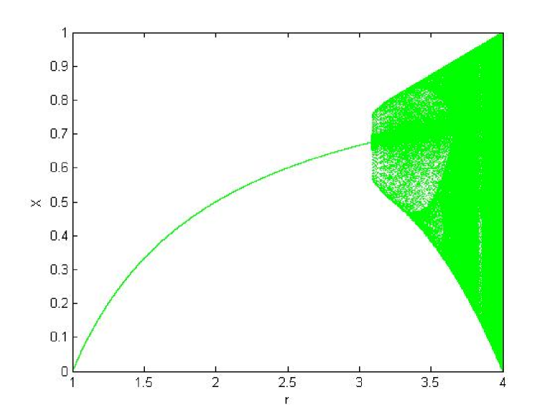
Figure 3: Bifurcation diagram for increasing $r$, with $a=1$, $x_{0}=\frac{r-1}{r}$, $y_{0}=0$ and $z_{0}=0$.

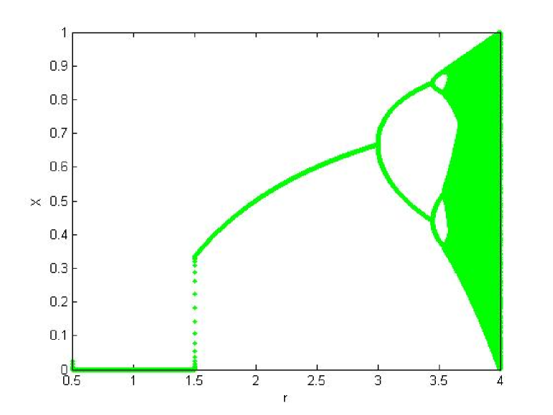
Figure 4: Bifurcation diagram for $r=4$, with $a=1$, $x_{0}=0.19$, $y_{0}=0.105$ and $z_{0}=0.352$.

Figure 5: Bifurcation diagram for increasing $\beta$, with $r=4$, $x_{0}=0.2$, $y_{0}=0$ and $z_{0}=0$.