Dynamical eigenfunctions and critical density
in loop quantum cosmology

Abstract

We offer a new, physically transparent argument for the existence of the critical, universal maximum matter density in loop quantum cosmology for the case of a flat Friedmann-Lemaître-Robertson-Walker cosmology with scalar matter. The argument is based on the existence of a sharp exponential ultraviolet cutoff in momentum space on the eigenfunctions of the quantum cosmological dynamical evolution operator (the gravitational part of the Hamiltonian constraint), attributable to the fundamental discreteness of spatial volume in loop quantum cosmology. The existence of the cutoff is proved directly from recently found exact solutions for the eigenfunctions for this model. As a consequence, the operators corresponding to the momentum of the scalar field and the spatial volume approximately commute. The ultraviolet cutoff then implies that the scalar momentum, though not a bounded operator, is in effect bounded on subspaces of constant volume, leading to the upper bound on the expectation value of the matter density. The maximum matter density is universal (i.e. independent of the quantum state) because of the linear scaling of the cutoff with volume. These heuristic arguments are supplemented by a new proof in the volume representation of the existence of the maximum matter density. The techniques employed to demonstrate the existence of the cutoff also allow us to extract the large-volume limit of the exact eigenfunctions, confirming earlier numerical and analytical work showing that the eigenfunctions approach superpositions of the eigenfunctions of the Wheeler-DeWitt quantization of the same model. We argue that generic (not just semiclassical) quantum states approach symmetric superpositions of expanding and contracting universes.

I Introduction

Loop quantized cosmological models generically predict that the “big bang” of classical general relativity is replaced by a quantum “bounce” in the deep-Planckian regime, at which the density of matter is bounded by a maximum density, typically called the “critical density” $\rho_{\textit{crit}}$. (See Refs. Ashtekar and Singh (2011); Bojowald (2011) for recent reviews of loop quantum cosmology [LQC] and what is currently known about these bounds in various models, as well as references to the earlier literature.) In most models, the value of this critical density is inferred from numerical simulations of quasiclassical states. So far it has been possible in only a single model – the exactly solvable loop quantization, dubbed “sLQC” Ashtekar et al. (2008), of a flat Friedmann-Lemaître-Robertson-Walker cosmology sourced by a massless, minimally coupled scalar field – to demonstrate analytically the existence of $\rho_{\textit{crit}}$ for generic quantum states. In this model, it was shown that $\rho_{\textit{crit}}\approx 0.41\rho_{p}$, where $\rho_{p}$ is the Planck density. As in other models, the bound for the density was first found numerically in Refs. Ashtekar et al. (2006a, b). This value was then confirmed and given a clean analytic proof in Ref. Ashtekar et al. (2008).

In this paper we offer a new demonstration of the existence of a critical density in this model with the hope of enriching the understanding of existing results. The argument is rooted in a study of the behavior of the dynamical eigenfunctions of the model’s evolution operator, the gravitational part of the Hamiltonian constraint, based on an explicit analytical solution for these eigenfunctions found recently in Refs. Ashtekar et al. (2010a, b). We will show from this solution that the eigenfunctions exhibit an exponential cutoff in momentum space that is proportional to the spatial volume. This ultraviolet cutoff may be understood as a consequence of the fundamental discreteness of spatial volume exhibited by these models. As a consequence of the cutoff, the quantum operators corresponding to the scalar momentum and spatial volume approximately commute. The ultraviolet cutoff then implies that the scalar momentum – even though its spectrum is not bounded – is in effect bounded on subspaces of constant volume. The proportionality of the cutoff to the spatial volume then leads to the existence of a critical density that is universal in the sense that it is independent of the quantum state.

It has long been understood in the loop quantum cosmology community that the behavior of the eigenfunctions of the gravitational Hamiltonian constraint operator is the key to understanding the physics of loop quantum models. In particular, the quantum “repulsion” generated by quantum geometry at small volume – leading to the signature quantum bounce – was clearly recognized in the decay of the eigenfunctions at small volume in many examples Ashtekar et al. (2006a, b). (See also e.g. Refs. Ashtekar et al. (2007); Bentivegna and Pawlowski (2008); Kamiński and Pawlowski (2010), among many others.) It was also recognized numerically that the onset of this decay as a function of volume depended linearly on the constraint eigenvalue. (See e.g. Refs. Ashtekar et al. (2007); Bentivegna and Pawlowski (2008).) What is new in this work is the shift in focus to the behavior of the eigenfunctions as functions of the continuous variable $k$ labeling the constraint/momentum eigenvalues. This allows certain insights that may not be as evident when they are considered as functions of the discrete volume variable $\nu$. From the exact solutions for the eigenfunctions of sLQC, we are able to show a genuinely exponential cutoff in the eigenfunctions as functions of $k$ that sets in at a value of $k$ that is proportional to the spatial volume, thus confirming and grounding the numerical observations analytically. This, of course, is the same cutoff that manifests as the decay of the eigenfunctions at small volume, considered as functions of the volume – this is clearly evident in, for example, Fig. 3 – but seen from a complementary perspective that is in some ways cleaner because of the continuous nature of the variable $k$. From there, we go on to show how the linear scaling of the cutoff gives rise to the universal upper limit on the matter density. To our knowledge, this connection between the linear scaling of the cutoff on the eigenfunctions and the existence and value of the universal critical density has not previously been noted.

Though appealingly intuitive, this argument is essentially heuristic, so we supplement it with a new proof in the volume representation of the existence of a $\rho_{\textit{crit}}$ in this model. (The proof of Ref. Ashtekar et al. (2008) is in a different representation of the physical operators.)

Thus we are able to offer a clear physical and mathematical account of the origin and value of the critical density, grounded analytically in the exact solutions for this model, that complements and confirms extensive numerical and analytic results extant in the literature. This perspective may be of some use in numerical and analytical investigations into the existence of a critical density in more complex models for which full analytical solutions are not available. We expand on this point in the discussion at the end, after we have developed the necessary details.

As a by-product of the methods employed to reveal the ultraviolet cutoff on the dynamical eigenfunctions, the semi-classical (large volume) limit of the eigenfunctions is also obtained from the exact eigenfunctions. The result confirms the essence of the result obtained on the basis of analytical and numerical considerations in Refs. Ashtekar et al. (2006a, b), that the exact eigenfunctions approach a linear combination of the eigenfunctions for the Wheeler-DeWitt quantization of the same physical model. (See also Ref. Kamiński and Pawlowski (2010), in which a careful analysis of the asymptotic limit of solutions to the gravitational constraint arrived at the same result as demonstrated here from the explicit solutions for the eigenfunctions.) The domain of applicability of this approximation is described. This result is then used to argue that, in the limit of large spatial volume, generic states in LQC – not just quasiclassical ones – become symmetric superpositions (in a precise sense to be specified) of expanding and contracting universes. The symmetry exhibited in numerical evolutions of semiclassical states – see e.g. Refs. Ashtekar et al. (2006a, b, 2008); Ashtekar and Singh (2011) – is therefore not an artifact of semiclassicality, but a generic property of all states in loop quantum cosmology. (Compare Refs. Corichi and Singh (2008); Kamiński and Pawlowski (2010) for analytic results bounding dispersions of states, showing they remain small on both sides of the bounce.)

The plan of the paper is as follows. In Sec. II we summarize the loop quantization of a flat FLRW spacetime sourced by a massless scalar field. Sec. III studies the dynamical eigenfunctions $e^{(s)}_{k}(\nu)$ of the model in detail, exhibiting various explicit forms for the solutions, and works out the asymptotic behavior of the $e^{(s)}_{k}(\nu)$ in the limits $|\nu|\gg\lambda|k|$ and $\lambda|k|\gg|\nu|$, where $\lambda$, defined in Eq. (7), is related to the LQC “area gap”. (The ultraviolet cutoff on the $e^{(s)}_{k}(\nu)$ emerges from this analysis in Sec. III.1.3.) In Sec. III.2 the cutoff is employed to place bounds on the matrix elements of the physical operators and argue that the scalar momentum is approximately diagonal in the volume representation. Section IV applies these results to show that generic states in sLQC are symmetric superpositions of expanding and contracting Wheeler-DeWitt universes at large volume. Finally, Sec. V offers an intuitive argument for the existence of a critical density in this model based on the UV cutoff for the eigenfunctions, as well as a new analytic proof in the volume representation. Section VI closes with some discussion.

II Flat scalar FRW and its loop quantization

In this section we briefly describe the loop quantization of a flat ($k=0$) Friedmann-Robertson-Walker universe with a massless, minimally coupled scalar field as a matter source. The model is worked out in detail in Refs. Ashtekar et al. (2006a, b, 2008) (see also Ref. Livine and Martín-Benito (2012)); see Ref. Ashtekar et al. (2010a) for a summary with a useful perspective and Refs. Ashtekar and Singh (2011); Bojowald (2011) for recent general reviews of results concerning loop quantizations of cosmological models.

II.1 Classical homogeneous and isotropic models

The starting point is a flat, fiducial metric $\mathring{q}_{ab}$ on a spatial manifold $\Sigma$ in terms of which the physical 3-metric is given by $q_{ab}=a^{2}\,\mathring{q}_{ab}$, where $a$ is the scale factor. The full metric is given by

$$g_{ab}=-n_{a}n_{b}+q_{ab},$$ (1)

where the normal $n_{a}=-N\,dt_{a}$ to the fixed (${\mathcal{L}}_{t}\mathring{q}_{ab}=0$) spatial slices is given in terms of a global time $t$ and lapse $N(t)$, so that $a=a(t)$.

For the Hamiltonian formulation of the quantum theory spatial integrals over a finite volume are required. We may therefore either choose $\Sigma$ to have topology $\mathbb{T}^{3}$ with volume $\mathring{V}$ with respect to $\mathring{q}_{ab}$, or topology $\mathbb{R}^{3}$ and choose a fixed fiducial cell ${\mathcal{V}}$, also with volume $\mathring{V}$ with respect to $\mathring{q}_{ab}$. The choice plays no role in the sequel and we will proceed in the language of the latter choice. The physical volume of ${\mathcal{V}}$ is therefore $V=a^{3}\,\mathring{V}$.

For a massless, minimally coupled scalar field, after the integration over the spatial cell ${\mathcal{V}}$ has been carried out the classical action is

$$S=\mathring{V}\int dt\left\{-\frac{3}{8\pi G}\frac{a\dot{a}^{2}}{N}+\frac{1}{2}a^{3}\frac{\dot{\phi}^{2}}{N}\right\}.$$ (2)

The classical Hamiltonian is thus

$$H=\frac{1}{\mathring{V}}\left\{-\frac{2\pi G}{3}\frac{N}{a}p_{a}^{2}+\frac{1}{2}\frac{N}{a^{3}}p_{\phi}^{2}\right\},$$ (3)

where $p_{a}$ and $p_{\phi}$ are the canonical momenta conjugate to the scale factor and scalar field.

Solving Hamilton’s equations yields the classical dynamical trajectories, for which $p_{\phi}$ is a constant of the motion, and

$$\phi=\pm\,\frac{1}{\sqrt{12\pi G}}\,\ln\left|\frac{V}{V_{o}}\right|+\phi_{o},$$ (4)

where $V_{o}$ and $\phi_{o}$ are constants of integration. Regarding the value of the scalar field $\phi$ as an emergent internal physical “clock”, the classical trajectories correspond to disjoint expanding ($+$) and contracting ($-$) branches. The expanding branch has a past singularity (the big bang) in the limit $\phi\rightarrow-\infty$, and the contracting branch a future singularity (big crunch) as $\phi\rightarrow+\infty$. (See Fig. 1.) Note that all classical solutions of this model are singular in one of these limits.

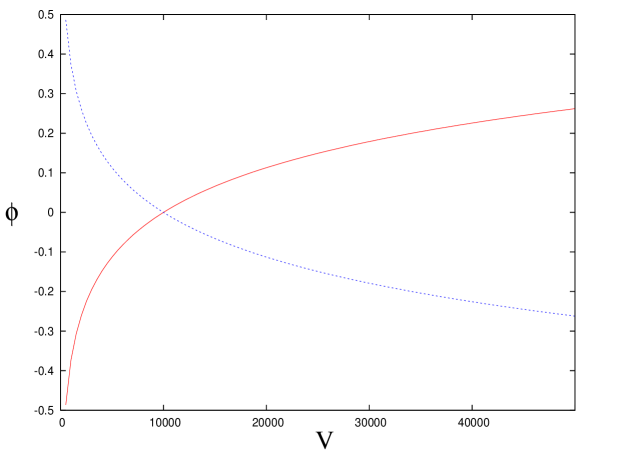
Figure 1: Two classical trajectories (Eq. (4)) for a massless scalar field in a flat homogeneous isotropic universe are shown. The solid (red) curve corresponds to an expanding branch and the dashed (blue) curve to the corresponding disjoint contracting branch. The branches are singular in the “past” and “future” given by the internal time $\phi$, respectively. (Figure taken from Ref. Craig and Singh (2010).)

Finally, we observe that the matter density $\rho$ on the spatial slices $\Sigma$ at scalar field value $\phi$ is given in the classical theory by the ratio of the energy in the scalar field to the volume at that $\phi$:

$$\rho|_{\phi}=\frac{p_{\phi}^{2}}{2V|_{\phi}^{2}}.$$ (5)

Here $\rho=T_{ab}u^{a}u^{b}$, where $u^{a}=(d/d\tau)^{a}$ and $d\tau=N\,dt$.

II.2 Loop quantization

In the quantum theory, following Ref. Ashtekar et al. (2008) we will discuss volume in terms of the variable $\nu$,

$$\nu=\varepsilon\frac{V}{2\pi\gamma l_{p}^{2}},$$ (6)

where $\gamma$ is the Barbero-Immirzi parameter, $l_{p}=\sqrt{G\hbar}$ is the Planck length (we take $c=1$), and $\varepsilon=\pm 1$ determines the orientation of the physical triad relative to the fiducial (co-)triad $\mathring{\omega}^{i}_{a}$ determining $\mathring{q}_{ab}$ ($=\mathring{\omega}^{i}_{a}\mathring{\omega}^{j}_{b}\delta_{ij}$) – see Refs. Ashtekar et al. (2006a, b, 2008); Ashtekar and Singh (2011). Thus $-\infty<\nu<+\infty$. Note that $\nu$ is dimensionful. For comparison to other work, note that $\nu=\lambda\cdot v$, where $v$ is the dimensionless volume variable of Refs. Ashtekar et al. (2006a, b), and

$$\lambda = \sqrt{\Delta}\cdot l_{p}$$ (7a)

$$= \sqrt{4\sqrt{3}\pi\gamma}\cdot l_{p}.$$ (7b)

Here $\Delta\cdot l_{p}^{2}$ is the “area gap” of loop quantum gravity.

Remarkably, when the physical model given by Eq. (2) is loop-quantized in these variables, the classical “harmonic” gauge choice $N(t)=a(t)^{3}$ leads to an exactly solvable quantum theory, referred to as “sLQC” (for “solvable LQC”) Ashtekar et al. (2008); Ashtekar and Singh (2011). One finds that physical states $\Psi(\nu,\phi)$ may be chosen to be “positive frequency” solutions to the quantum constraint,

$$-i\partial_{\phi}\Psi(\nu,\phi)=\sqrt{\smash[b]{\Theta_{\nu}}}\Psi(\nu,\phi),$$ (8)

where the positive, self-adjoint “evolution operator” $\Theta$ (the quantized gravitational constraint) is given in the $\nu$-representation by a second-order difference operator,

$$(\Theta\Psi)(\nu,\phi)=-\frac{3\pi G}{4\lambda^{2}}\left\{\sqrt{|\nu(\nu+4\lambda)|}|\nu+2\lambda|\Psi(\nu+4\lambda,\phi)-2\nu^{2}\Psi(\nu,\phi)\right.\\ \left.+\sqrt{|\nu(\nu-4\lambda)|}|\nu-2\lambda|\Psi(\nu-4\lambda,\phi)\right\}.$$ (9)

Solutions to the full quantum constraint ($\hat{\mathcal{C}}=-[\partial_{\phi}^{2}+\Theta]$) therefore decompose into disjoint sectors with support on the $\epsilon$-lattices given by $\nu=4\lambda n+\epsilon$, where $\epsilon\in[0,4\lambda)$ Ashtekar et al. (2006a, b). In order not to exclude the classical singularity at $\nu=0$ from the start, we work exclusively on the lattice $\epsilon=0$, so that in this quantum cosmological model, the volume is discrete:

$$\nu=4\lambda n,\qquad n\in\mathbb{Z}.$$ (10)

Group averaging yields the physical inner product

$$\langle{\Psi}\!\mid\!{\Phi}\rangle=\sum_{\nu=4\lambda n}\Psi(\nu,\phi_{o})^{*}\Phi(\nu,\phi_{o})$$ (11)

for some fiducial (but irrelevant) $\phi_{o}$. According to Eq. (8), states at different values of the scalar field $\phi$ may be mapped onto one another by the unitary evolution

$$\Psi(\nu,\phi)=e^{i\sqrt{\smash[b]{\Theta_{\nu}}}(\phi-\phi_{o})}\,\Psi(\nu,\phi_{o}),$$ (12)

It is natural therefore – though not essential Ashtekar et al. (2006a) – to regard the scalar field $\phi$ as an emergent physical “clock” or “internal time” in which states evolve in this model. Eq. (12) shows that the inner product of Eq. (11) is independent of the choice of $\phi_{o}$, and is therefore preserved under evolution from one $\phi$-“slice” to another.

Finally, we note that in the absence of fermions, the action, dynamics, and other physics of the model are insensitive to the orientation of the physical triads Ashtekar et al. (2006a, b, 2008); Martín-Benito et al. (2009). We may therefore restrict attention to the volume-symmetric sector of the theory in which

$$\Psi(\nu,\phi)=\Psi(-\nu,\phi).$$ (13)

Many further details concerning the quantization of this model and its observables may be found in Refs. Ashtekar et al. (2006a, b, 2008); Ashtekar and Singh (2011); Livine and Martín-Benito (2012).

II.3 Observables

The basic variables in this representation are the scalar field $\phi$ and the volume $\nu$. Employing $\phi$ as an internal time, the primary operators of interest are the volume, which acts as a multiplication operator,

$$\hat{\nu}\,\Psi(\nu,\phi) = \nu\,\Psi(\nu,\phi),$$ (14a)

$$\hat{V}\,\Psi(\nu,\phi) = 2\pi\gamma l_{p}^{2}\,|\nu|\,\Psi(\nu,\phi),$$ (14b)

and the scalar momentum $\hat{p}_{\phi}$,

$$\hat{p}_{\phi}\,\Psi(\nu,\phi) = -i\hbar\,\partial_{\phi}\Psi(\nu,\phi)$$ (15a)

$$= \hbar\sqrt{\smash[b]{\Theta_{\nu}}}\,\Psi(\nu,\phi).$$ (15b)

(In this paper we will not have need of the (exponential of the) momentum $\boldsymbol{\mathrm{b}}$ conjugate to $\nu$ Ashtekar et al. (2006a, b).) As in the classical theory, the scalar momentum $\hat{p}_{\phi}$ is a constant of the motion – it obviously commutes with the effective “dynamics” given by $\sqrt{\Theta}$ – and is therefore a Dirac observable. The volume $\hat{\nu}$ is not, but the corresponding “relational” observable $\hat{\nu}|_{\phi^{*}}$ giving the volume at a fixed value $\phi^{*}$ of the internal time $\phi$ is. Defining

$$U(\phi)=e^{i\sqrt{\Theta}\phi},$$ (16)

the “Heisenberg” operator $\hat{\nu}|_{\phi^{*}}(\phi)$ acting on states at $\phi$ is given by

$$\hat{\nu}|_{\phi^{*}}(\phi)=U(\phi^{*}-\phi)^{\dagger}\hat{\nu}U(\phi^{*}-\phi),$$ (17)

so that, for example, the physical volume $\hat{V}=2\pi\gamma l_{p}^{2}\,|\hat{\nu}|$ of the cell ${\mathcal{V}}$ at $\phi^{*}$ is given by the operator

$$\hat{V}|_{\phi^{*}}(\phi)\,\Psi(\nu,\phi)=2\pi\gamma l_{p}^{2}e^{i\sqrt{\smash[b]{\Theta_{\nu}}}(\phi-\phi^{*})}|\nu|\Psi(\nu,\phi^{*}).$$ (18)

It is straightforward to verify that $\hat{p}_{\phi}$ and $\hat{V}|_{\phi^{*}}(\phi)$ commute with $U(\phi)$, and are therefore Dirac observables.

III Eigenfunctions of the evolution operator

General physical states $\Psi(\nu,\phi)$ may be readily expressed in terms of the eigenfunctions of the dynamical evolution operator $\Theta$ – the gravitational part of the Hamiltonian constraint – given by

$$\Theta_{\nu}e_{k}(\nu)=\omega_{k}^{2}\,e_{k}(\nu),$$ (19)

where

$$\omega_{k} = \sqrt{12\pi G}\,|k|$$ (20a)

$$\equiv \kappa\,|k|,$$ (20b)

and $-\infty<k<\infty$ is a dimensionless number labelling the 2-fold degenerate eigenvalues. Restricting to the symmetric lattice $\nu=4\lambda n$ and physical states which satisfy Eq. (13), we usually choose to work with a symmetric basis of eigenfunctions $e^{(s)}_{k}(\nu)$ which satisfy $e^{(s)}_{k}(\nu)=e^{(s)}_{k}(-\nu)$. In terms of these physical states may be expressed simply as

$$\Psi(\nu,\phi)=\int_{-\infty}^{+\infty}dk\,\tilde{\Psi}(k)\,e^{(s)}_{k}(\nu)\,e^{i\omega_{k}\phi}.$$ (21)

For normalized states, $\sum_{\nu=4\lambda n}|\Psi(\nu,\phi)|^{2}=1$,

$$\int_{-\infty}^{+\infty}dk\,|\tilde{\Psi}(k)|^{2}=1.$$ (22)

Explicit analytic expressions for the eigenfunctions of $\Theta$ have recently been found Ashtekar et al. (2010a, b). The symmetric eigenfunctions will eventually be expressed in terms of the primitive eigenfunctions Ashtekar et al. (2010a)

$$e_{0}(\nu) = \delta_{0,\nu}$$ (23a)

$$e_{k}(\nu) = A(k)\sqrt{\frac{\lambda|\nu|}{\pi}}\int_{0}^{\pi/\lambda}db\,e^{-i\frac{\nu b}{2}}e^{ik\ln(\tan\frac{\lambda b}{2})}\qquad(k\neq 0),$$ (23b)

where $A(k)$ is a normalization factor which for consistency will always be chosen to be

$$A(k)=\frac{1}{\sqrt{4\pi k\sinh(\pi k)}}.$$ (24)

The functions $e_{k}(\nu)$ have support on both positive and negative $\nu$ and are not symmetric in $\nu$. It is convenient to seek linear combinations $e^{\pm}_{k}(\nu)$ of $e_{k}(\nu)$ and $e_{-k}(\nu)$ which have support only for $\nu\gtrless 0$. The correct combinations turn out to be Ashtekar et al. (2010a)

$$e^{\pm}_{k}(\nu)=\frac{1}{2}\left\{e^{\pm\frac{\pi k}{2}}e_{k}(\nu)+e^{\mp\frac{\pi k}{2}}e_{-k}(\nu)\right\}.$$ (25)

Clearly $\sum_{\nu}e^{\pm}_{k}(\nu)^{*}e^{\mp}_{k^{\prime}}(\nu)=0$. The choice of $A(k)$ in Eq. (24) corresponds to the normalization

$$\sum_{\nu=4\lambda n}e^{\pm}_{k}(\nu)^{*}e^{\pm}_{k^{\prime}}(\nu)=\delta^{(s)}(k,k^{\prime}),$$ (26)

where $\delta^{(s)}(k,k^{\prime})$ is the symmetric delta distribution

$$\delta^{(s)}(k,k^{\prime})=\frac{1}{2}\left\{\delta(k,k^{\prime})+\delta(k,-k^{\prime})\right\}.$$ (27)

(In contrast to Ref. Ashtekar et al. (2010a), we choose to work with the full range of $k$, $-\infty<k<\infty$. This leads to the second delta function appearing in Eq. (26) relative to Eq. (C13) of that reference. Since as we will see these functions are symmetric in $k$, the two approaches are of course equivalent, but do lead to some differences in choices of normalization.)

The $e^{\pm}_{k}(\nu)$ can be given explicitly as Ashtekar et al. (2010a)

$$e^{\pm}_{k}(\nu) = A(k)\sqrt{\frac{\pi|\nu|}{\lambda}}I(k,\pm\nu/4\lambda)$$ (28a)

$$= A(k)\sqrt{\frac{\pi|\nu|}{\lambda}}I(k,\pm n),$$ (28b)

recalling $\nu=4\lambda n$. Here $I(k,n)=0$ for $n<0$, and for $n\geq 0$ is given by

$$I(k,n) = ik\sum_{m=0}^{2n}\frac{1}{m!(2n-m)!}\prod_{l=1}^{2n-1}(ik+m-l)$$ (29a)

$$= -ik\frac{\Gamma(2n-ik)}{\Gamma(1+2n)\Gamma(1-ik)}\,_{2}F_{1}(ik,-2n;1-2n+ik;-1),$$ (29b)

where the second form follows from the first by simple manipulations of the definition of the hypergeometric function ${}_{2}F_{1}(a,b;c;z)$ Abramowitz and Stegun (1964).

We will discuss the properties of $I(k,n)$ in detail later. For now, note from Eq. (28) that

$$e^{\pm}_{k}(-\nu)=e^{\mp}_{k}(\nu),$$ (30)

and from Eq. (25) that

$$e^{\pm}_{-k}(\nu)=e^{\pm}_{k}(\nu).$$ (31)

Given the symmetry relation Eq. (30) it is clear that the symmetric eigenfunctions $e^{(s)}_{k}(\nu)$ are finally

$$e^{(s)}_{k}(\nu) = \frac{1}{\sqrt{2}}\left\{e^{+}_{k}(\nu)+e^{-}_{k}(\nu)\right\}$$ (32a)

$$= A(k)\sqrt{\frac{\pi|\nu|}{2\lambda}}\ I(k,|\nu|/4\lambda)$$ (32b)

$$= \sqrt{\frac{|n|}{2|k\sinh(\pi k)|}}\ I(k,|n|).$$ (32c)

The following symmetry properties may be verified:

$$e^{(s)}_{k}(-\nu) = e^{(s)}_{k}(\nu)$$ (33a)

$$e^{(s)}_{-k}(\nu) = e^{(s)}_{k}(\nu)$$ (33b)

$$e^{(s)}_{k}(\nu)^{*} = e^{(s)}_{k}(\nu).$$ (33c)

The $e^{(s)}_{k}(\nu)$ with $A(k)$ chosen as in Eq. (24) then satisfy the completeness relations

$$\sum_{\nu=4\lambda n}e^{(s)}_{k}(\nu)^{*}e^{(s)}_{k^{\prime}}(\nu) = \delta^{(s)}(k,k^{\prime})$$ (34a)

$$\int_{-\infty}^{+\infty}dk\,e^{(s)}_{k}(\nu)e^{(s)}_{k}(\nu^{\prime})^{*} = \delta^{(s)}_{\nu,\nu^{\prime}},$$ (34b)

where the symmetric Kronecker delta is defined analogously to Eq. (27). (The domains of these expressions are understood to be even functions of $k$ and $\nu$, respectively.) The symmetrized deltas arise because the functions $e^{(s)}_{k}(\nu)$ are symmetric in both $\nu$ and $k$.

An expression for $e^{(s)}_{k}(\nu)$ we will find useful later is

$$e^{(s)}_{k}(\nu)=\frac{\cosh(\pi k/2)}{\sqrt{2}}\left\{e_{k}(\nu)+e_{-k}(\nu)\right\},$$ (35)

which follows from Eqs. (32a) and (25). As a useful aside, note it is easy to see from Eq. (23) that $e^{(s)}_{k}(\nu)^{*}=e^{(s)}_{-k}(-\nu)$. Additionally, the change of variable $b^{\prime}=-b+\pi/\lambda$ in Eq. (23) – remembering $\nu=4\lambda n$ – reveals that

$$e_{k}(-\nu)=e_{-k}(\nu).$$ (36)

Thus $e_{k}(\nu)^{*}=e_{-k}(-\nu)=e_{k}(\nu)$, and both $e_{k}(\nu)$ and $e^{(s)}_{k}(\nu)$ are therefore real.

This completes the catalog of properties of the eigenfunctions we will require. We now describe the behavior of the functions $e^{(s)}_{k}(\nu)$ we seek to explain in the sequel. The results of the analysis will confirm and complement the understanding of earlier numerical and analytical work arrived at prior to the discovery of the exact solutions for this model.

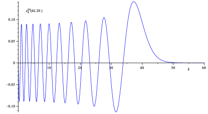
(a) $n=20$

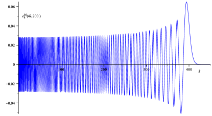
(b) $n=200$

Figure 2: Plot of $e^{(s)}_{k}(\nu=4\lambda n)$ as a function of $k\geq 0$ for $n=20$ and $n=200$. Regarded as a function of $k$, $e^{(s)}_{k}(\nu)$ is symmetric in $k$ and always exhibits exactly $n-1$ nodes in addition to the node at $k=0$. The largest zero and last maximum of $e^{(s)}_{k}(\nu)$ always appears at a value $|k_{\textit{max}}|\lesssim 2|n|$, after which $e^{(s)}_{k}(\nu)$ is exponentially damped in $k$. This ultraviolet cutoff at $|k|=2|n|=|\nu/2\lambda|$ in the eigenfunctions will be explained analytically in the sequel.

Plots of $e^{(s)}_{k}(\nu)$ are shown in Figs. 2, 3 and 4. Two behaviors are clearly evident in these plots. First, the dynamical eigenfunctions are exponentially damped as functions of $k$ for $|k|>2|n|=|\nu/2\lambda|$ (Figs. 2-3). This is the ultraviolet momentum space cutoff in the eigenfunctions described in the introduction. The cutoff can be understood as a consequence of the fundamental discreteness of volume in these quantum theories. Second, for $|n|>|k|$, the eigenfunctions $e^{(s)}_{k}(\nu)$ settle quickly into a decaying sinusoidal oscillation in $n$ (Fig. 4). We will see that this oscillation corresponds to a specific symmetric superposition of the eigenfunctions for the Wheeler-DeWitt quantization of the same physical model. As a consequence, generic quantum states in this loop quantum cosmology will evolve to a symmetric superposition of an expanding and a collapsing Wheeler-DeWitt universe.

Figure 3: Plot of the functions $e^{(s)}_{k}(\nu=4\lambda n)$ in the $(k,n)$ plane for $0\leq n\leq 75$ and $|k|<75$. They are symmetric in both $k$ and $n$. The volume variable $\nu=4\lambda n$ is fundamentally discrete; the values of the eigenfunctions are plotted as continuous in both variables $k$ and $n$ for reasons of visual clarity only. (The functions $e^{(s)}_{k}(\nu)$ were evaluated only at integer values of $n$ to construct this surface, of course.) The plots in Fig. 2 showing the dependence of the $e^{(s)}_{k}(\nu)$ on $k$ at fixed $n$ may be viewed as constant-$n$ cross-sections of this surface. Similarly, Fig. 4, showing the dependence of the $e^{(s)}_{k}(\nu)$ on $n$ at fixed $k$, may be viewed as constant-$k$ cross-sections of this surface. The exponential ultraviolet cutoff along the lines $|k|=2|n|=|\nu/2\lambda|$ is clearly evident. The dynamical eigenfunctions $e^{(s)}_{k}(\nu)$ may therefore be regarded to an excellent approximation as having support only in the “wedge” $|k|\lesssim 2|n|$. It is this feature of the eigenfunctions that is ultimately responsible for the existence of a universal upper bound to the matter density.

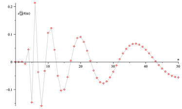
(a) $k=10$

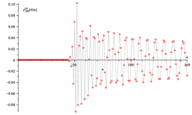
(b) $k=100$

Figure 4: Plot of $e^{(s)}_{k}(\nu=4\lambda n)$ as a function of $n\geq 0$ for $k=10$ and $k=100$. Regarded as a function of $n\in\mathbb{Z}$, the $e^{(s)}_{k}(\nu)$ are symmetric in $n$ and have support only on the lattice $\nu=4\lambda n$; the points are connected for visual clarity only. Note $e^{(s)}_{k}(0)=0$ for $k\neq 0$. The functions $e^{(s)}_{k}(\nu=4\lambda n)$ for fixed $k$ decay rapidly to essentially zero for $|n|\lesssim|k|/2$, the ultraviolet cutoff in the eigenfunctions also visible in Figs. 4-3. (The cutoff is not as sharp viewed on slices of constant $k$ as it is on slices of constant $n$, on which the cutoff is truly exponential.) For $|n|\gtrsim|k|/2$, they settle rapidly into a regular decaying oscillation. This latter behavior corresponds precisely to a symmetric superposition of Wheeler-DeWitt eigenfunctions to be elaborated in the sequel.

III.1 Asymptotics

It is evident from Fig. 3 that, to an excellent approximation, the dynamical eigenfunctions $e^{(s)}_{k}(\nu)$ may be regarded as having support only in the wedge $|k|\lesssim 2|n|$ in the $(k,n)$ plane. We now seek to explain this behavior based on an analysis of the exact solutions, Eq. (32), as well as the large volume limit and other features visible in Figs. 2-4.

From Eqs. (32) and (29), $e^{(s)}_{k}(\nu)$ is given by $\sqrt{|n|/2|k\cdot\sinh(\pi k)|}$ times the polynomial $I(k,|n|)$. Indeed, examination of $I(k,|n|)$, regarded as a polynomial in $k$, shows that it is an even polynomial in $k$ with no constant term, whose terms alternate in sign. Thus we see immediately that $e^{(s)}_{k}(0)=0$ and $e^{(s)}_{0}(\nu)=0$ for $\nu\neq 0$ (cf. Eq. (23a)). Examination of plots of $I(k,|n|)$ (as in Fig. 2) shows that it always exhibits the maximum number of roots possible $(2n-1)$ for such a polynomial; the alternating signs of the coefficients lead to the oscillations.

Writing the product in Eq. (29a) as a “falling factorial” Abramowitz and Stegun (1964), it is possible to arrive at an explicit expression for $I(k,|n|)$ which is useful for some computations:

$$I(k,|n|)=\sum_{j=1}^{|n|}a(|n|,j)\,k^{2j},$$ (37)

where the coefficients $a(|n|,j)$ are given by

$$a(n,j)=(-1)^{j}\sum_{l=2j}^{2n}s(2n-1,l-1)\cdot\binom{l-1}{2j-1}\cdot\left(\sum_{m=0}^{2n}\frac{(m-1)^{l-2j}}{m!(2n-m)!}\right).$$ (38)

Here the $s(p,q)$ denote the (signed) Stirling numbers of the first kind. It should be noted that the factor to the right of $(-1)^{j}$ is always positive, leading to the alternating signs of these coefficients.

For large $|k|$, $I(k,|n|)$ is dominated by $k^{2|n|}$, and therefore

$$e^{(s)}_{k}(\nu=4\lambda n) \sim \frac{1}{\sqrt{k\sinh(\pi k)}}\cdot k^{2|n|}$$ (39a)

$$\sim |k|^{2n-\frac{1}{2}}\cdot e^{-\pi k/2},$$ (39b)

and the decay of the eigenfunctions is indeed exponential in $k$ past the largest root of $e^{(s)}_{k}(\nu)$.

III.1.1 Steepest descents

To identify the value of $k$ at which the decay of the symmetric eigenfunctions $e^{(s)}_{k}(\nu)$ sets in requires a bit more work. Recall from Eq. (35) that the $e^{(s)}_{k}(\nu)$ may be expressed in terms of the primitive eigenfunctions $e_{k}(\nu)$ given by Eq. (23). The integral in this equation is of the form

$${\mathcal{I}}(k,\nu)=\int_{0}^{\frac{\pi}{\lambda}}db\ e^{if(b,k,\nu)},$$ (40)

where

$$f(b,k,\nu)=k\cdot\ln(\tan\frac{\lambda b}{2})-\frac{\nu b}{2}.$$ (41)

This was the form from which the exact expression Eq. (28) was extracted in Ref. Ashtekar et al. (2010a). We however wish to evaluate this integral in the limits of large $|k|$ and $|\nu|$. While Eq. (40) is not quite of the same form for which the steepest descents approximation is normally discussed – a single large parameter multiplying an overall phase – the same arguments for the validity of the approximation apply. In regions where $f(b,k,\nu)$ is large, the integrand oscillates rapidly and contributions from neighboring values of $b$ cancel one another. The dominant contributions to ${\mathcal{I}}(k,\nu)$, therefore, come from regions close to the stationary points of $f(b,k,\nu)$ where $f$ changes only slowly with $b$ and the cancellations are not strong. This is the usual steepest-descents approximation, and in general one has Dennery and Krzywicki (1995)

$$\int dz\,e^{if(z)}g(z)\approx\sum_{i}\sqrt{\frac{2\pi}{|f^{\prime\prime}(z_{i})|}}\,e^{if(z_{i})}\,g(z_{i})\,e^{i\frac{\pi}{4}\operatorname{sgn}(f^{\prime\prime}(z_{i}))},$$ (42)

where the $z_{i}$ locate the stationary points $f^{\prime}(z_{i})=0$ along the relevant contour.

It is clear that when $|k|$ or $|\nu|$ are large, $f(b,k,\nu)$ can become large, suppressing the value of ${\mathcal{I}}(k,\nu)$, and so we seek the stationary points of $f$.

First observe that $f(b,k,\nu)$ diverges at $b=0$ and $b=\pi/\lambda$, so there is no contribution to ${\mathcal{I}}(k,\nu)$ from the endpoints of the integration due to the rapid oscillation of the integrand there. Next, one finds

$$\frac{\partial f}{\partial b}(b,k,\nu)=\frac{\lambda k}{\sin\lambda b}-\frac{\nu}{2}$$ (43)

and

$$\frac{\partial^{2}f}{\partial b^{2}}(b,k,\nu)=-\frac{\lambda^{2}k\cos\lambda b}{\sin^{2}\lambda b}.$$ (44)

The stationary points therefore satisfy

$$\sin\lambda b=\frac{2\lambda k}{\nu}.$$ (45)

When solutions exist there are two roots $b_{1}$ and $b_{2}$, given in the limit $|\nu|\gg\lambda|k|$ by

$$b_{1} \approx \frac{2k}{\nu},$$ (46a)

$$b_{2} \approx \frac{\pi}{\lambda}-\frac{2k}{\nu}.$$ (46b)

In this limit

$$f(b_{1},k,\nu) \approx -k\left[\ln\frac{\nu}{\lambda k}+1\right],$$ (47a)

$$f(b_{2},k,\nu) \approx +k\left[\ln\frac{\nu}{\lambda k}+1\right]-\frac{\pi\nu}{2\lambda},$$ (47b)

and

$$\frac{\partial^{2}f}{\partial b^{2}}(b_{1},k,\nu) \approx -\frac{\nu^{2}}{4k},$$ (48a)

$$\frac{\partial^{2}f}{\partial b^{2}}(b_{2},k,\nu) \approx +\frac{\nu^{2}}{4k}.$$ (48b)

We now piece together these results to study the asymptotic limits of ${\mathcal{I}}(k,\nu)$ and consequently $e^{(s)}_{k}(\nu)$.

III.1.2 Wheeler-DeWitt limit

We will begin by considering the case in which $k$ and $\nu$ are both positive, and return to the other possibilities shortly. When $\nu\gg\lambda k>0$, from Eq. (42) we find

$${\mathcal{I}}(k,\nu) \approx \sqrt{\frac{2\pi}{|f^{\prime\prime}(b_{1})|}}\,e^{if(b_{1})}\,e^{i\frac{\pi}{4}\operatorname{sgn}(f^{\prime\prime}(b_{1}))}+\sqrt{\frac{2\pi}{|f^{\prime\prime}(b_{2})|}}\,e^{if(b_{2})}\,e^{i\frac{\pi}{4}\operatorname{sgn}(f^{\prime\prime}(b_{2}))}$$ (49a)

$$\cong \sqrt{\frac{8\pi|k|}{\nu^{2}}}\left\{e^{-ik\left[\ln\frac{\nu}{\lambda k}+1\right]}e^{-i\frac{\pi}{4}}+e^{+ik\left[\ln\frac{\nu}{\lambda k}+1\right]}e^{+i\frac{\pi}{4}}e^{-i\frac{\pi\nu}{2\lambda}}\right\}$$ (49b)

$$= 2\sqrt{\frac{8\pi|k|}{\nu^{2}}}\cos\left(k\left[\ln\frac{\nu}{\lambda k}+1\right]+\frac{\pi}{4}\right),$$ (49c)

where to get to the last line we recall $\nu=4\lambda n$, so the final exponential factor in Eq. (49b) is unity.

In the case where $k$ and $\nu$ are both negative, the same results obtain, but now

$$f(b_{1},k,\nu) \approx +|k|\left[\ln\frac{\nu}{\lambda k}+1\right]\phantom{-\frac{\pi\nu}{2\lambda}}\qquad\ \operatorname{sgn}(f^{\prime\prime}(b_{1}))=+,$$ (50a)

$$f(b_{2},k,\nu) \approx -|k|\left[\ln\frac{\nu}{\lambda k}+1\right]-\frac{\pi\nu}{2\lambda}\qquad\operatorname{sgn}(f^{\prime\prime}(b_{2}))=-,$$ (50b)

again leading to a cosine, but with $k\rightarrow|k|$. Thus, from Eqs. (23), (24), and (49c), we find

$$e_{k}(\nu)\cong\frac{2}{\sqrt{|\sinh(\pi k)}|}\sqrt{\frac{2\lambda}{\pi|\nu|}}\cos\left(|k|\ln\left|\frac{\nu}{\lambda}\right|+\alpha(|k|)\right)\text{ when }\left\{\begin{array}[]{lcl}|\nu|\gg\lambda|k|\\ \nu\cdot k>0\end{array}\right.,$$ (51)

where

$$\alpha(k)=k(1-\ln k)+\frac{\pi}{4}.$$ (52)

We have yet to consider the case where $k$ and $\nu$ are opposite in sign. In this case note that since $0\leq b\leq\pi/\lambda$, there are no solutions to Eq. (45), and $f(b,k,\nu)$ has no stationary points in the domain of integration. Thus ${\mathcal{I}}(k,\nu)$, and hence $e_{k}(\nu)$, are strongly suppressed by the rapid oscillations of the integrand when $k$ and $\nu$ are opposite in sign.

We note from Eq. (35) that the symmetric eigenfunctions $e^{(s)}_{k}(\nu)$ are a linear combination of $e_{k}(\nu)$ and $e_{-k}(\nu)$. The functions $e_{-k}(\nu)$ are, mutatis mutandis as above, strongly suppressed when $\nu$ and $k$ have the same sign, and assume the limit Eq. (51) when $k$ and $\nu$ are opposite in sign. The $|\nu|\gg\lambda|k|$ limit of $e^{(s)}_{k}(\nu)$ will therefore pick up precisely one contribution of the form of Eq. (51) no matter the signs of $k$ and $\nu$. Observing that $\cosh(\pi k/2)/\sqrt{\sinh(\pi|k|)}\approx 1/\sqrt{2}$ for even very modest values of $k\gtrsim 1$, we arrive finally at

$$e^{(s)}_{k}(\nu)\cong\sqrt{\frac{2\lambda}{\pi|\nu|}}\cos\left(|k|\ln\left|\frac{\nu}{\lambda}\right|+\alpha(|k|)\right)\qquad|\nu|\gg\lambda|k|.$$ (53)

Fig. 5 shows that the exact eigenfunctions settle down to this asymptotic form very quickly. We will employ Eq. (53) to study in Sec. IV the large volume limit of flat scalar loop quantum universes.

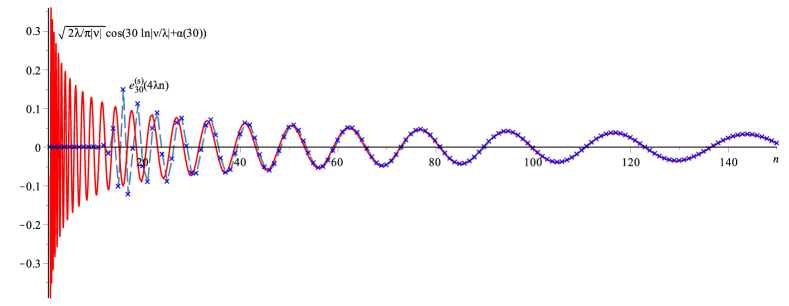
Figure 5: Plot as a function of $n$ of both the dynamical eigenstate $e^{(s)}_{k}(\nu=4\lambda n)$ and the asymptotic form Eq. (53) for $k=30$. The volume variable $\nu=4\lambda n$ is fundamentally discrete; the values of $e^{(s)}_{k}(n)$ are marked with blue ${\scriptstyle\times}$’s; the points are connected by a dashed blue line for visual clarity. The solid red curve is the corresponding asymptotic form. The rapid convergence to the asymptotic form for $|n|\gg|k|$ on the lattice $\nu=4\lambda n$ is clear. Note this asymptotic form corresponds to the particular superposition of eigenstates of the Wheeler-DeWitt quantization of the same model given by Eq. (69). The rapid oscillations visible at small volume are the correct physical behavior of the Wheeler-DeWitt states, and are ultimately responsible for the fact that these models are singular in the Wheeer-DeWitt quantization. See Refs. Craig and Singh (2010, 2013) for further discussion.

The asymptotic expression Eq. (53) was, in effect, arrived at on the basis of analytical and numerical considerations in Ref. Ashtekar et al. (2006b), with a numerically motivated fit for the phase $\alpha(k)$. In Ref. Kamiński and Pawlowski (2010) an expression equivalent to Eq. (53) was derived from a careful analysis of the asymptotic limit of solutions to the constraint equation, including an expression for the phase $\alpha(k)$ equivalent to Eq. (52). (See Ref. Martín-Benito et al. (2009) for a related analysis of this limit.) Here we have instead derived this asymptotic form from the exact eigenfunctions, explicitly confirming these prior analyses with the exact solutions for the model.

III.1.3 Ultraviolet Cutoff

Figures 2-3 clearly exhibit the exponential ultraviolet cutoff in the eigenfunctions $e^{(s)}_{k}(\nu)$ for values of $|k|>2|n|=|\nu/2\lambda|$. We know already from Eq. (39) that an exponential decay will eventually set in. The only question is, at what value of $k$ does that occur? We have, in fact, already seen the origin of this cutoff and its value. Eq. (45) shows that $f(b,k,|\nu|)$ has no stationary points when $|2\lambda k/\nu|>1$. In other words, ${\mathcal{I}}(k,\nu)$, hence $e_{k}(\nu)$ and $e^{(s)}_{k}(\nu)$, are strongly suppressed unless

$$|k| \lesssim \left|\frac{\nu}{2\lambda}\right|$$ (54a)

$$= 2|n|.$$ (54b)

This cutoff – in particular, its linear scaling with volume – may be understood physically as a consequence of the underlying discreteness of the quantum geometry. States with wave numbers $|k|>2|n|$ (i.e. wavelengths shorter than the scale set by $|\lambda/\nu|$) are not supported. Alternately, it may be viewed as the manifestation in the eigenfunctions of the “quantum repulsion” generated by quantum geometry at volumes smaller than the wave number.

III.1.4 Small volume limit

The same argument shows that the eigenstates will, equivalently, decay rapidly for small volume, when $|n|\lesssim|k|/2$, as is clear in Fig. 4. Eq. (39) tells us the decay in $e^{(s)}_{k}(\nu)$ as a function of $k$ is exponential. The precise functional form of the decay as a function of $n$ is less evident, but the figures show it is also quick.

At this point a comment may be in order. It is tempting to study this question by regarding $e^{(s)}_{k}(\nu)$ as a function of a continuous variable $\nu$. However, plotting the exact expressions for $e^{(s)}_{k}(\nu)$ for continuous values of $\nu$ on top of the values for $\nu=4\lambda n$ should quickly disabuse one of the notion that there is a simple sense in which $e^{(s)}_{k}(\nu)$ is well approximated by its naive continuation to the continuum. In fact, as discussed in detail in Ref. Ashtekar et al. (2008), the convergence to the Wheeler-DeWitt theory in the continuum is not uniform, and must be extracted with some care in the limit the “area gap” set by $\lambda$ – fixed in loop quantum cosmology to the value of Eq. (7) – tends to 0.

As noted in the Introduction, and as is clearly evident in Fig. 3, the ultraviolet cutoff in momentum space is the “same” cutoff as the rapid decay at small volume as a function of volume that has long been known in loop quantum cosmology based on numerical solutions for the eigenfunctions Ashtekar et al. (2006a, b). It was also known numerically that the onset of this decay was proportional to the eigenvalue $\omega_{k}$. (See e.g. Refs. Ashtekar et al. (2007); Bentivegna and Pawlowski (2008).) What is new in the present work, facilitated by the change in perspective to consideration of the behavior of the eigenfunctions as functions of the continuous variable $k$, is an analytic understanding of the linear cutoff grounded in a study of the model’s exact solutions, its precise value, and its specific relation to the critical density.

III.2 Representation of operators

As noted above in Eq. (13), we have restricted attention to the volume-symmetric sector of the theory. This is only possible because the physical operators preserve the symmetry of the quantum states.

From Eq. (9), the matrix elements of $\Theta$ in the volume basis may be expressed as

$$\langle{\nu}|{\Theta}|{\nu^{\prime}}\rangle=12\pi G\sqrt{|n\cdot n^{\prime}|}|n+n^{\prime}|\cdot\left\{\delta_{n,n^{\prime}}-\frac{1}{2}\left[\delta_{n,n^{\prime}+1}+\delta_{n,n^{\prime}-1}\right]\right\},$$ (55)

where $\nu=4\lambda n$ and $\nu^{\prime}=4\lambda n^{\prime}$. Note these matrix elements satisfy the following properties:

$$\langle{\nu}|{\Theta}|{\nu}\rangle = \langle{-\nu}|{\Theta}|{-\nu}\rangle$$ (56a)

$$\langle{\nu}|{\Theta}|{\nu^{\prime}}\rangle = \langle{\nu}|{\Theta}|{\nu^{\prime}}\rangle^{*}$$ (56b)

$$= \langle{\nu^{\prime}}|{\Theta}|{\nu}\rangle.$$ (56c)

Owing to these relations, the operator $\Theta$ preserves the subspaces ${\mathcal{H}}_{\mathrm{phys}}^{(s)}$ and ${\mathcal{H}}_{\mathrm{phys}}^{(a)}$ of states that are even and odd in $\nu$, so that $P^{(s)}\Theta P^{(a)}=0$, where $P^{(s)}$ and $P^{(a)}$ are the corresponding projections. (In other words, $\Theta$ commutes with the parity operator $\Pi_{\nu}=P^{(s)}-P^{(a)}$ Ashtekar et al. (2006a, b).) On the symmetric subspace ${\mathcal{H}}_{\mathrm{phys}}^{(s)}$ to which we have restricted ourselves, $\Theta|_{{\mathcal{H}}_{\mathrm{phys}}^{(s)}}=P^{(s)}\Theta P^{(s)}\equiv\Theta^{(s)}$ (and correspondingly $p_{\phi}^{(s)}=\hbar\sqrt{\Theta^{(s)}}$) may be decomposed in terms of the symmetric basis of eigenstates $|{k^{(s)}}\rangle$,

$$\Theta^{(s)}=\kappa^{2}\int dk\,k^{2}|{k^{(s)}}\rangle\langle{k^{(s)}}|,$$ (57)

where $e^{(s)}_{k}(\nu)\equiv\langle{\nu}\!\mid\!{k^{(s)}}\rangle$. The matrix elements of $\Theta^{(s)}$ in the volume representation are related to those of $\Theta$ by

$$\langle{\nu}|{\Theta^{(s)}}|{\nu^{\prime}}\rangle = \frac{1}{2}\left\{\langle{\nu}|{\Theta}|{\nu^{\prime}}\rangle+\langle{\nu}|{\Theta}|{-\nu^{\prime}}\rangle\right\}$$ (58a)

$$= \langle{\nu}|{\Theta^{(s)}}|{-\nu^{\prime}}\rangle.$$ (58b)

The actions of $\Theta$ and $\Theta^{(s)}$ on ${\mathcal{H}}_{\mathrm{phys}}^{(s)}$ are of course completely equivalent. Since $\hat{p}_{\phi}^{2}=\hbar^{2}\Theta$ on ${\mathcal{H}}_{\mathrm{phys}}$, these expressions give the matrix elements of $\hat{p}_{\phi}^{2}$ on ${\mathcal{H}}_{\mathrm{phys}}^{(s)}$ as well.

The matrix elements of $\hat{p}_{\phi}=\hbar\sqrt{\Theta}$ are more complex. These are given in terms of derivatives of a generating function in Appendix C of Ref. Ashtekar et al. (2010a). Explicit expressions for the physical observables in another representation are also given in Ref. Ashtekar et al. (2008). Here we note that on ${\mathcal{H}}_{\mathrm{phys}}^{(s)}$ we may employ the $e^{(s)}_{k}(\nu)$ to calculate $\hat{p}^{(s)}_{\phi}$ explicitly in the volume representation. Indeed, the polynomial solution Eq. (37) for $I(k,n)$ makes it a straightforward matter to evaluate these matrix elements. The result is (with $\nu=4\lambda n$ and $\nu^{\prime}=4\lambda m$)

$$\int_{-\infty}^{\infty}\!dk\,|k|\,e^{(s)}_{k}(\nu)e^{(s)}_{k}(\nu^{\prime})^{*}=\\ \sqrt{|n\cdot m|}\,\sum_{j=1}^{|n|}\sum_{l=1}^{|m|}a(|n|,j)a(|m|,l)\frac{2^{2(j+l)+1}-1}{2^{2(j+l)}\pi^{2(j+l)+1}}\Gamma(2(j+l)+1)\zeta(2(j+l)+1)\\ \approx\sqrt{|n\cdot m|}\,\sum_{j=1}^{|n|}\sum_{l=1}^{|m|}a(|n|,j)a(|m|,l)\frac{2}{\pi^{2(j+l)+1}}\Gamma(2(j+l)+1),$$ (59)

where $\zeta(z)$ is the Riemann zeta-function. This expression gives the $(\nu,\nu^{\prime})$ matrix elements of $\hat{p}^{(s)}_{\phi}/\hbar\kappa$, or equivalently $\smash{\sqrt{\Theta^{(s)}}}/\kappa$.

We observe from Eq. (55) that $\Theta$ is nearly diagonal in the volume representation, with only the $n^{\prime}=n,n\pm 1$ elements not exactly zero. The same is therefore true of $\hat{p}_{\phi}^{2}$. Direct numerical evaluation of the expression Eq. (59) reveals that $\hat{p}_{\phi}$ – and therefore $\sqrt{\Theta}$ – are also nearly diagonal in the volume representation, with only the $n^{\prime}=n,n\pm 1$ matrix elements significantly different from zero. (See Fig. 6.) In this case, however, the off-diagonal elements of $\hat{p}_{\phi}$ are merely very small, rather than precisely zero.

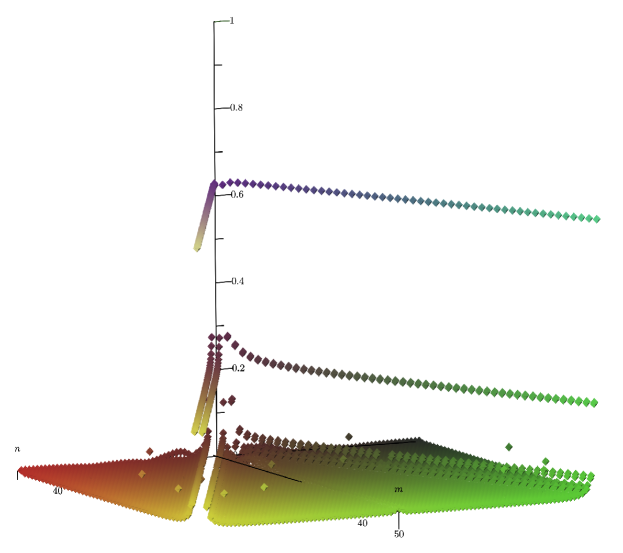
Figure 6: Plot of the norm of the scalar momentum matrix element overlap integral appearing in Eq. (63) normalized by the estimated maximum value $\tfrac{1}{2}|\nu/2\lambda|=|n|$ of this integral on the diagonal $|\nu|=|\nu^{\prime}|$, taking $|\nu=4\lambda n|\leq|\nu^{\prime}=4\lambda m|$: $|\int_{-\infty}^{\infty}dk|k|e^{(s)}_{k}(\nu)e^{(s)}_{k}(\nu^{\prime})^{*}|/|n|$. The integrals have been calculated numerically from the exact eigenfunctions over the range $0<|n|\leq 50$ and $0<m\leq 50$. According to the upper bound expressed in Eq. (62), this normalized matrix element is bounded above by one, and as argued is strongly suppressed off the diagonal $|\nu|=|\nu^{\prime}|$. In effect, these plots show that $\hat{p}_{\phi}$ approximately commutes with $|\hat{\nu}|$ since it is nearly diagonal in the $\nu$-representation. This is essentially the reason the “moral” argument expressed in Eq. (84) for the existence of a critical density in this model yields the correct result.

The values of these matrix elements can be understood as a consequence of the ultraviolet cutoff, Eq. (54). Indeed, the exponential cutoff $|k|\lesssim|\nu/2\lambda|$ implies that the diagonal matrix elements are bounded,

$$\int_{-\infty}^{\infty}\!dk\,|k|\,e^{(s)}_{k}(\nu)e^{(s)}_{k}(\pm\nu)^{*}\lesssim\frac{1}{2}\left|\frac{\nu}{2\lambda}\right|.$$ (60)

(The $1/2$ is a consequence of the symmetric normalization of the eigenfunctions, Eq. (34).) This bound on $\smash{\sqrt{\Theta^{(s)}}}/\kappa$ may be compared with that set by the exact expression for $\Theta$, Eq. (55). From Eq. (58),

$$\langle{\nu}|{\Theta^{(s)}}|{\nu}\rangle = \frac{1}{2}\langle{\nu}|{\Theta}|{\nu}\rangle$$ (61a)

$$= \frac{\kappa^{2}}{4}\left|\frac{\nu}{2\lambda}\right|^{2}.$$ (61b)

As it is always the case that $\langle{\hat{A}^{2}}\rangle\geq\langle{\hat{A}}\rangle^{2}$, we see that a strict bound on the diagonal matrix elements of $\smash{\sqrt{\Theta^{(s)}}}/\kappa$ is

$$\int_{-\infty}^{\infty}\!dk\,|k|\,e^{(s)}_{k}(\nu)e^{(s)}_{k}(\pm\nu)^{*}\leq\frac{1}{2}\left|\frac{\nu}{2\lambda}\right|,$$ (62)

in agreement with the bound inferred from the UV cutoff.

The off-diagonal elements may be bounded in a similar manner. For simplicity assume $|\nu|<|\nu^{\prime}|$. The exponential UV cutoff effectively restricts the range of integration to $|k|\lesssim|\nu/2\lambda|$. The Cauchy-Schwarz inequality then gives

$$\left|\int_{-\infty}^{\infty}\!dk\,|k|e^{(s)}_{k}(\nu)e^{(s)}_{k}(\nu^{\prime})^{*}\right|\lesssim\left|\frac{\nu}{2\lambda}\right|\sqrt{\int_{-|\nu/2\lambda|}^{|\nu/2\lambda|}\!dk\,|e^{(s)}_{k}(\nu)|^{2}}\sqrt{\int_{-|\nu/2\lambda|}^{|\nu/2\lambda|}\!dk\,|e^{(s)}_{k}(\nu^{\prime})|^{2}}.$$ (63)

Again, because the $e^{(s)}_{k}(\nu)$ are symmetrically normalized, the value of the first square root is essentially $1/\sqrt{2}$. As for the second, we note from Fig. 2 that the $e^{(s)}_{k}(\nu)$ execute approximately uniform amplitude oscillations, growing slowly with increasing $k$ with a short lived increase before the exponential cutoff sets in at $|k|=|\nu/2\lambda|$. Therefore, for $|\nu|<|\nu^{\prime}|$ we may estimate that at most

$$\int_{-|\nu/2\lambda|}^{|\nu/2\lambda|}\!dk\,|e^{(s)}_{k}(\nu^{\prime})|^{2}\lesssim\frac{1}{2}\left|\frac{\nu}{\nu^{\prime}}\right|,$$ (64)

showing that the cutoff alone implies that the off-diagonal terms are suppressed relative to the diagonal terms. Interference effects only reduce their values further; Fig. 6 shows that except for the $n=n^{\prime}\pm 1$ elements – as with $\Theta$ itself – this suppression is dramatic.

As a shorthand to express these bounds, we can say that $\hat{p}_{\phi}$ and $|\hat{\nu}|$ – and therefore $|\hat{\nu}|_{\phi}$ – approximately commute, in the sense that $\langle{\nu}|{\hat{p}_{\phi}}|{\nu^{\prime}}\rangle$ is approximately diagonal. (See Fig. 6.) We will see in Sec. V that this helps explain why the matter density in these models remains bounded even though the spectrum of the scalar momentum $\hat{p}_{\phi}$ is not itself bounded.

IV Large volume limit of loop quantum states

In Eq. (53) we have exhibited the large volume (more precisely, $|\nu|\gg\lambda|k|$) limit of the basis $e^{(s)}_{k}(\nu)$ of symmetric states of flat scalar loop quantum cosmology. We extracted this limit from the exact solution for the model’s eigenfunctions, essentially confirming prior numerical and analytical work. In this section we relate these states to the eigenstates in a Wheeler-DeWitt quantization of the same physical model.

A complete, rigorous Hilbert space quantization of a flat Friedmann-Lemaître-Robertson-Walker cosmology sourced by a massless minimally coupled scalar field has been given in Refs. Ashtekar et al. (2006a, b) and compared to its loop quantization in detail in Ref. Ashtekar et al. (2008). It is known rigorously that states in the Wheeler-DeWitt quantization are generically singular just as they are in the classical theory in the sense that all states assume arbitrarily small volume (equivalently, large density) at some point in their cosmic evolution in “internal time” $\phi$ Ashtekar et al. (2008); Craig and Singh (2010).

The classical solutions are given in Eq. (4), corresponding to disjoint expanding and contracting branches which either begin or end in the classical singularity at $V=0$. Solutions to the Wheeler-DeWitt quantum theory similarly divide into disjoint expanding and contracting branches, and as noted, are singular in the same way.

The Wheeler-DeWitt version of the quantum constraint is Ashtekar et al. (2006b)

$$\partial_{\phi}^{2}\Psi^{{\scriptscriptstyle\text{WdW}}}(\nu,\phi) = 12\pi G\frac{1}{\sqrt{|\nu|}}\ \nu\partial_{\nu}(\nu\partial_{\nu}\sqrt{|\nu|}\Psi^{{\scriptscriptstyle\text{WdW}}}(\nu,\phi))$$ (65a)

$$:= \Theta^{{\scriptscriptstyle\text{WdW}}}_{\nu}\Psi^{{\scriptscriptstyle\text{WdW}}}(\nu,\phi).$$ (65b)

Attention may again be restricted to symmetric (Eq. (13)), positive frequency solutions in the sense of Eq. (8). The symmetric eigenstates of $\Theta^{{\scriptscriptstyle\text{WdW}}}_{\nu}$ satisfying Eqs. (19)-(20) are

$$e^{{\scriptscriptstyle\text{WdW}}}_{k}(\nu)=\frac{1}{\sqrt{4\pi|\nu|}}e^{ik\ln\left|\frac{\nu}{\lambda}\right|},$$ (66)

and are orthonormal (distributionally normalized to $\delta(k,k^{\prime})$) in the inner product

$$\langle{\Psi^{{\scriptscriptstyle\text{WdW}}}}\!\mid\!{\Phi^{{\scriptscriptstyle\text{WdW}}}}\rangle=\int_{-\infty}^{\infty}d\nu\,\Psi^{{\scriptscriptstyle\text{WdW}}}(\nu,\phi)^{*}\Phi^{{\scriptscriptstyle\text{WdW}}}(\nu,\phi)$$ (67)

resulting from group averaging. Physical states may then be expressed as

$$\Psi^{{\scriptscriptstyle\text{WdW}}}(\nu,\phi) = \int_{-\infty}^{+\infty}dk\,\tilde{\Psi}^{{\scriptscriptstyle\text{WdW}}}(k)\,e^{{\scriptscriptstyle\text{WdW}}}_{k}(\nu)\,e^{i\omega_{k}\phi}$$

$$= \frac{1}{\sqrt{4\pi|\nu|}}\int_{-\infty}^{0}dk\,\tilde{\Psi}^{{\scriptscriptstyle\text{WdW}}}(k)\,e^{ik\left[\ln\left|\frac{\nu}{\lambda}\right|-\kappa\phi\right]}$$

$$\qquad+\frac{1}{\sqrt{4\pi|\nu|}}\int_{0}^{\infty}dk\,\tilde{\Psi}^{{\scriptscriptstyle\text{WdW}}}(k)\,e^{ik\left[\ln\left|\frac{\nu}{\lambda}\right|+\kappa\phi\right]}$$ (68b)

$$\equiv \Psi^{{\scriptscriptstyle\text{WdW}}}_{R}(\nu,\phi)+\Psi^{{\scriptscriptstyle\text{WdW}}}_{L}(\nu,\phi).$$ (68c)

The orthogonal sectors of “right-moving” (in a plot of $\phi$ vs. $\nu$) and “left-moving” states clearly correspond to the expanding and contracting branches of the classical solutions, Eq. (4). A priori, note that $\tilde{\Psi}^{{\scriptscriptstyle\text{WdW}}}_{R}(k)=\tilde{\Psi}^{{\scriptscriptstyle\text{WdW}}}(k)\ (k<0)$ and $\tilde{\Psi}^{{\scriptscriptstyle\text{WdW}}}_{L}(k)=\tilde{\Psi}^{{\scriptscriptstyle\text{WdW}}}(k)\ (k>0)$ need not be in any way related in the Wheeler-DeWitt theory.

We now show that generic states in the loop quantized theory decompose into symmetric superpositions of expanding and collapsing (right- and left-moving) Wheeler-DeWitt universes at large volume. This follows simply from Eq. (53), which may be written

$$e^{(s)}_{k}(\nu)\cong z\sqrt{\lambda}\left\{e^{{\scriptscriptstyle\text{WdW}}}_{+|k|}(\nu)e^{+i\alpha(|k|)}+e^{{\scriptscriptstyle\text{WdW}}}_{-|k|}(\nu)e^{-i\alpha(|k|)}\right\}\qquad|\nu|\gg 2\lambda|k|,$$ (69)

where $z=\sqrt{2}$ for the normalization of Eq. (66) appropriate to the range $-\infty<\nu<\infty$ of Eq. (67), and the $\sqrt{\lambda}$ is present because the $e^{(s)}_{k}(\nu)$ are dimensionless, whereas the $e^{{\scriptscriptstyle\text{WdW}}}_{k}(\nu)$ are not. The factor of $z\sqrt{\lambda}$ can be understood as arising from the difference between normalization of the Wheeler-DeWitt eigenfunctions on the continuous range $-\infty<\nu<\infty$ vs. the normalization of loop quantum states on an infinite lattice with step-size $4\lambda$. (Compare Appendix B of Ref. Kamiński and Pawlowski (2010).)

The relationship expressed in Eq. (69) has long been known in loop quantum cosmology on the basis of both analytic and numerical arguments. See, for example, Eq. (5.3) of Ref. Ashtekar et al. (2006b), as well as Eq. (3.1) of Ref. Kamiński and Pawlowski (2010) – which also contains a careful analysis of the convergence properties of this limit – among many others. Here we have confirmed that the asymptotic behavior of the exact solutions agrees precisely with these earlier arguments.

We know that the limit Eq. (69) is valid when $|\nu|\gg 2\lambda|k|$, and more generally, that $e^{(s)}_{k}(\nu)$ has support only in the wedge $|k|\lesssim|\nu|/2\lambda$. Eq. (69) therefore holds inside this wedge of support but clearly breaks down near its boundary $|k|=2|n|$. From Eq. (21), quite generally

$$\Psi(\nu,\phi) = \int_{-\infty}^{\infty}dk\ \tilde{\Psi}(k)e^{(s)}_{k}(\nu)e^{i\omega_{k}\phi}$$ (70a)

$$\cong \int_{-|\nu|/2\lambda}^{|\nu|/2\lambda}dk\ \tilde{\Psi}(k)e^{(s)}_{k}(\nu)e^{i\omega_{k}\phi}.$$ (70b)

It is noted in Ref. Kamiński and Pawlowski (2010) that one must take care to draw conclusions concerning the asymptotic behavior of states in sLQC based on that of the eigenfunctions because the convergence of the sLQC basis $e^{(s)}_{k}(\nu)$ to that of the Wheeler-DeWitt theory is not uniform in $k$. Nonetheless, we argue that for a wide class of quantum states, there will be a well-defined region depending on the state in which this approximation will hold for that state.

Specifically, replacement of $e^{(s)}_{k}(\nu)$ in the expression Eq. (70) with its asymptotic form Eq. (69) will be valid for values of the volume (significantly larger than that) for which the Fourier transform $\tilde{\Psi}(k)$ does not have significant support outside the wedge at that volume. Quantum states are normalized, so we know that $\tilde{\Psi}(k)$ is square-integrable. Because functions of compact support are dense in $L^{2}(\mathbb{R})$, there is a dense set of states for which, for every state $\Psi(\nu,\phi)$ in this set, there is some value of $|k|$ whose value will in general depend on the state – call it $k_{\Psi}$ – outside of which $\tilde{\Psi}(k)$ has no support. Therefore, for a dense set of states in the quantum theory the replacement Eq. (69) will be a good approximation for $|\nu|\gg 2\lambda|k_{\Psi}|$. It is worth emphasizing, therefore, that the domain of applicability of the large-volume approximation is dependent upon the quantum state through the support of $\tilde{\Psi}(k)$.

For states satisfying this condition and within that domain of applicability, we may write

$$\Psi(\nu,\phi)\cong z\sqrt{\lambda}\int_{-|\nu|/2\lambda}^{|\nu|/2\lambda}dk\ \tilde{\Psi}(k)\left\{e^{{\scriptscriptstyle\text{WdW}}}_{+|k|}(\nu)e^{+i\alpha(|k|)}+e^{{\scriptscriptstyle\text{WdW}}}_{-|k|}(\nu)e^{-i\alpha(|k|)}\right\}e^{i\kappa|k|\phi}.$$ (71)

It will be seen shortly that the first term corresponds to a contracting universe, and the second, expanding. To begin, we note from Eqs. (20), (21), and (33b) that $\tilde{\Psi}(k)$ is even, $\tilde{\Psi}(-k)=\tilde{\Psi}(k)$. Consider the first term alone. As Eq. (71) applies only for values of the volume for which $\tilde{\Psi}(k)$ has negligible support for $|k|>|\nu|/2\lambda$, we may extend the range of $k$-integration to $-\infty<k<\infty$. By separating the integral $\int_{-\infty}^{\infty}dk=\int_{-\infty}^{0}dk+\int_{0}^{\infty}dk$ and making the change of variable $k^{\prime}=-k$ in the first, one quickly finds

$$z\sqrt{\lambda}\int_{-\infty}^{\infty}dk\ \tilde{\Psi}(k)\,e^{{\scriptscriptstyle\text{WdW}}}_{|k|}(\nu)e^{i\alpha(|k|)}e^{i\kappa|k|\phi} = 2z\sqrt{\lambda}\int_{0}^{\infty}dk\ \tilde{\Psi}(k)e^{i\alpha(|k|)}e^{{\scriptscriptstyle\text{WdW}}}_{k}(\nu)e^{i\kappa|k|\phi}$$ (72a)

$$= \Psi_{L}(\nu,\phi).$$ (72b)

As in the Wheeler-DeWitt case, Eq. (68), $\Psi_{L}(\nu,\phi)$ clearly corresponds to a contracting quantum universe, with equivalent Wheeler-DeWitt Fourier transform

$$\tilde{\Psi}^{{\scriptscriptstyle\text{WdW}}}_{L}(k)=\tilde{\Psi}(k)e^{i\alpha(|k|)}\qquad k>0.$$ (73)

In an exactly similar way, the second term in Eq. (71) is

$$\Psi_{R}(\nu,\phi)\equiv 2z\sqrt{\lambda}\int_{-\infty}^{0}dk\ \tilde{\Psi}(k)e^{-i\alpha(|k|)}e^{{\scriptscriptstyle\text{WdW}}}_{k}(\nu)e^{i\kappa|k|\phi},$$ (74)

which describes an expanding universe with equivalent Wheeler-DeWitt Fourier transform

$$\tilde{\Psi}^{{\scriptscriptstyle\text{WdW}}}_{R}(k)=\tilde{\Psi}(k)e^{-i\alpha(|k|)}\qquad k<0.$$ (75)

Therefore, for a dense set of quantum states and within the domain of applicability of the large volume approximation $|\nu|\gg 2\lambda|k_{\Psi}|$ for the state $\Psi(\nu,\phi)$, we may always write

$$\Psi(\nu,\phi)\cong\Psi_{R}(\nu,\phi)+\Psi_{L}(\nu,\phi)\qquad\mbox{\scriptsize$\begin{pmatrix}\text{large}\\ \text{volume}\end{pmatrix}.$}$$ (76)

Unlike the Wheeler-DeWitt case, however, $\Psi_{L}$ and $\Psi_{R}$ are not independent. In fact, owing to the symmetry of $\tilde{\Psi}(k)$ in the loop quantum case, the equivalent Wheeler-DeWitt Fourier transforms are essentially the same, having equal modulus $|\tilde{\Psi}_{L}(-k)|=|\tilde{\Psi}_{R}(k)|$ and a fixed phase relation given by $\exp(i\alpha(|k|))$ between them. (Note that expressions equivalent to Eqs. (73) and (75) may also be found in Ref. Kamiński and Pawlowski (2010). These relations are central to the “scattering” picture of loop quantum cosmology developed in that reference.)

Thus, we have shown from the exact solution that in the sense given by Eq. (76), at sufficiently large volume a dense set of states in flat scalar loop quantum cosmology may be written as symmetric superpositions of expanding and contracting universes. This is an essential feature of loop quantum cosmology, deeply connected with the fact that these cosmologies are non-singular Martín-Benito et al. (2009) – all states “bounce” with a finite maximum matter density.

It was observed long ago from numerical solutions that semiclassical states “bounce” symmetrically, including the dispersions of these states Ashtekar et al. (2006a, b). Analytic bounds on the dispersions of all states in this model have been proved in Refs. Corichi and Singh (2008); Kamiński and Pawlowski (2010), in which further discussion of constraints on the sense in which such states are symmetric can also be found. (In this regard see also Refs. Livine and Martín-Benito (2012); Martín-Benito et al. (2009).) Here we have demonstrated the symmetry of generic states (not just quasiclassical ones) at large volume, in the sense of Eq. (76), directly from the exact solutions.

V Critical density and the ultraviolet cutoff

A significant part of the interest in loop quantum cosmology has arisen from the fact that loop quantization seems to robustly and generically resolve cosmological singularities; see Ref. Ashtekar and Singh (2011); Bojowald (2011) for recent overviews. This was noticed first in numerical results for semiclassical states Ashtekar et al. (2006a, b), subsequently observed in many other models (see e.g. Refs. Ashtekar et al. (2007); Bentivegna and Pawlowski (2008)), and finally proved analytically for all quantum states in the model described in this paper in Ref. Ashtekar et al. (2008). In that paper it is shown that the expectation value (and hence spectrum) of the matter density $\hat{\rho}|_{\phi}$ is bounded above by

$$\rho_{\text{crit}} = \frac{\sqrt{3}}{32\pi^{2}\gamma^{3}}\frac{1}{Gl_{p}^{2}}$$ (77a)

$$\approx 0.41\cdot\rho_{p},$$ (77b)

where $\rho_{p}$ is the Planck density and the value of the Barbero-Immirzi parameter $\gamma\approx 0.2375$ inferred from black hole thermodynamics has been used Ashtekar and Lewandowski (2004).

We argue here that the existence of a universal upper bound to the density may be traced to the ultraviolet cutoff for values of $|k|\gtrsim|\nu/2\lambda|$ on the eigenfunctions $e^{(s)}_{k}(\nu)$.

Classically, the matter density when the scalar field has value $\phi$ is given by the ratio of the energy in the scalar field to the volume,

$$\rho|_{\phi}=\frac{p_{\phi}^{2}}{2V|_{\phi}^{2}}.$$ (78)

In Ref. Ashtekar et al. (2008) it is argued that a suitable definition for the corresponding quantum mechanical observable is

$$\hat{\rho}|_{\phi}=\frac{1}{2}\hat{A}|_{\phi}^{2},$$ (79)

where

$$\hat{A}|_{\phi}\equiv\frac{1}{\sqrt{\smash[b]{\hat{V}|_{\phi}}}}\,\hat{p}_{\phi}\,\frac{1}{\sqrt{\smash[b]{\hat{V}|_{\phi}}}}.$$ (80)

Even though the spectrum of this operator is not yet known, an upper bound on the spectrum of $\hat{A}|_{\phi}$ places a bound on the spectrum of $\hat{A}|_{\phi}^{2}$, thence on $\hat{\rho}|_{\phi}$. Ref. Ashtekar et al. (2008) then observed that

$$\langle{\hat{A}|_{\phi}}\rangle_{\Psi} = \frac{\langle{\Psi}|{\hat{A}|_{\phi}}|{\Psi}\rangle}{\langle{\Psi}\!\mid\!{\Psi}\rangle}$$ (81a)

$$= \frac{\langle{\chi}|{\hat{p}_{\phi}}|{\chi}\rangle}{\langle{\chi}|{\hat{V}|_{\phi}}|{\chi}\rangle},$$ (81b)

where $|{\chi}\rangle$ is defined through $|{\Psi}\rangle=\sqrt{\smash[b]{\hat{V}|_{\phi}}}|{\chi}\rangle$. Thus, the expectation value of $\hat{A}|_{\phi}$ (in the state $|{\Psi}\rangle$) may be expressed as the ratio of expectation values of the momentum and volume (in the state $|{\chi}\rangle$). Even though the spectrum of $\hat{p}_{\phi}$ is not bounded, they go on to show analytically that this ratio is nonetheless bounded above by $\sqrt{3/4\pi\gamma^{2}G}/\lambda$ for all states in the domain of the physical observables, leading directly to the bound given by Eq. (77) on the density.

Alternately, one might choose to define

$$\hat{\rho}|_{\phi}=\frac{1}{2}\frac{1}{\hat{V}|_{\phi}}\hat{p}_{\phi}^{2}\frac{1}{\hat{V}|_{\phi}}.$$ (82)

A similar argument then shows

$$\langle{\hat{\rho}|_{\phi}}\rangle_{\Psi}=\frac{1}{2}\frac{\langle{\omega}|{\hat{p}_{\phi}^{2}}|{\omega}\rangle}{\langle{\omega}|{\hat{V}|_{\phi}^{2}}|{\omega}\rangle},$$ (83)

where now $|{\Psi}\rangle=\hat{V}|_{\phi}|{\omega}\rangle$. For convenience, we will adopt this latter definition of the density in the sequel.

V.1 Heuristic argument

We offer here a new perspective on the existence of a universal upper bound to the density by arguing that it can be seen as a consequence of the linear scaling of the ultraviolet cutoff in the $e^{(s)}_{k}(\nu)$ with volume, $|k|\lesssim|\nu/2\lambda|$. We offer both a new proof of the existence of a critical density in this model in the volume representation, as well as an heuristic argument that has a clear and intuitive interpretation, making it a simple matter to calculate the value of the critical density simply from the slope of the scaling of the ultraviolet cutoff.

In fact, heuristically speaking, using Eq. (83) we see that the UV cutoff $|k|\lesssim|\nu/2\lambda|$ implies that

$$\langle{\hat{\rho}|_{\phi}}\rangle_{\Psi} = \frac{1}{2}\frac{\langle{\hat{p}_{\phi}^{2}}\rangle_{\omega}}{\langle{\hat{V}|_{\phi}^{2}}\rangle_{\omega}}$$ (84a)

$$\sim \frac{1}{2}\frac{(\hbar\kappa|k|)^{2}}{\hat{V}|_{\phi}^{2}}$$ (84b)

$$\lesssim \frac{1}{2}\left(\frac{\hbar\kappa}{2\lambda}\right)^{2}\left(\frac{|\nu|}{2\pi\gamma l_{p}^{2}|\nu|}\right)^{2},$$ (84c)

identical to the rigorous bound on the density – Eq. (77) – found in Ref. Ashtekar et al. (2008). The linear scaling in the UV cutoff on the eigenfunctions thus, in this heuristic way, leads directly to the existence of the universal critical density. In particular, the slope of the scaling gives the value of the critical density correctly.

This “moral” argument is of course not rigorous since $\hat{p}_{\phi}$ and $\hat{\nu}|_{\phi}$ do not commute. There is, however, an interesting reason the “moral” argument works: as discussed in Sec. III.2, the scalar momentum $\hat{p}_{\phi}$ and volume $|\hat{\nu}|_{\phi}$ operators approximately commute, again as a consequence of the ultraviolet cutoff. Thus, also as a consequence of the ultraviolet cutoff, the operator $\hat{p}_{\phi}$ is, though its spectrum is not bounded, in effect bounded on subspaces of fixed volume. This leads immediately to the upper bound on the density, as in the “moral” argument above.

The intended meaning of these statements is the following. Because of the ultraviolet cutoff,

$$|\hat{p}_{\phi}e^{(s)}_{k}(\nu)| = \hbar\kappa|k|\cdot|e^{(s)}_{k}(\nu)|$$ (85a)

$$\lesssim \hbar\kappa\left|\frac{\nu}{2\lambda}\right|\cdot|e^{(s)}_{k}(\nu)|.$$ (85b)

Consider the subspace spanned by volume eigenstates with volume less than or equal to some ${\mathcal{V}}$. While this subspace is not strictly invariant under the action of the operator $\hat{p}_{\phi}$, it is approximately so because the off-diagonal matrix elements $\langle{\nu}|{\hat{p}_{\phi}}|{\nu^{\prime}}\rangle$ are strongly suppressed. The norm of states restricted to this subspace is $\lVert\chi\rVert_{{\mathcal{V}}}^{2}=\sum_{|\nu|\leq{\mathcal{V}}}|\chi(\nu)|^{2}$. Then we have

$$\lVert\hat{p}_{\phi}e^{(s)}_{k}(\nu)\rVert_{{\mathcal{V}}}^{2} = (\hbar\kappa|k|)^{2}\sum_{|\nu|\leq{\mathcal{V}}}|e^{(s)}_{k}(\nu)|^{2}$$ (86a)

$$\lesssim (\hbar\kappa)^{2}\left|\frac{{\mathcal{V}}}{2\lambda}\right|^{2}\sum_{|\nu|\leq{\mathcal{V}}}|e^{(s)}_{k}(\nu)|^{2}$$ (86b)

$$= (\hbar\kappa)^{2}\left|\frac{{\mathcal{V}}}{2\lambda}\right|^{2}\lVert e^{(s)}_{k}(\nu)\rVert_{{\mathcal{V}}}^{2}$$ (86c)

and we can see that $\hat{p}_{\phi}$ is in effect bounded on subspaces of volume less than a given value. Given Eq. (81) or (83), this helps explain why the heuristic argument above gives the correct value for the critical density.

V.2 Proof in the volume representation

To complete this heuristic argument we offer a new, alternative proof of the existence of a critical density in this model in the volume representation, using the definition Eq. (82) for the density. (The original proof of Ref. Ashtekar et al. (2008) is in a different representation of the quantum states and operators and employs the definition Eq. (79) for the density, though their proof works for either definition.)

The action of the gravitational constraint $\Theta$ in the volume representation, Eq. (9), may be written

$$(\Theta\omega)(\nu,\phi)=\frac{1}{2}\left(\frac{\kappa}{2\lambda}\right)^{2}\nu^{2}\left\{\omega(\nu,\phi)-\overline{\omega}(\nu,\phi)\right\},$$ (87)

where

$$\overline{\omega}(\nu,\phi)=\frac{1}{2}\left[\sqrt{\left|1+\frac{4\lambda}{\nu}\right|}\left|1+\frac{2\lambda}{\nu}\right|\omega(\nu+4\lambda,\phi)+\sqrt{\left|1-\frac{4\lambda}{\nu}\right|}\left|1-\frac{2\lambda}{\nu}\right|\omega(\nu-4\lambda,\phi)\right]$$ (88)

is approximately the average of the values of $\omega$ on either side of the volume $\nu$. In this notation,

$$\langle{\hat{p}_{\phi}^{2}}\rangle_{\omega} = \hbar^{2}\langle{\omega(\phi)}|{\Theta}|{\omega(\phi)}\rangle$$ (89a)

$$= \frac{1}{2}\left(\frac{\hbar\kappa}{2\lambda}\right)^{2}\sum_{\nu}\left\{\nu^{2}\omega(\nu,\phi)^{*}\omega(\nu,\phi)-\nu^{2}\omega(\nu,\phi)^{*}\overline{\omega}(\nu,\phi)\right\}$$ (89b)

$$= \frac{1}{2}\left(\frac{\hbar\kappa}{2\lambda}\right)^{2}\left\{\langle{\hat{\nu}|_{\phi}^{2}}\rangle_{\omega}-\sum_{\nu}\nu^{2}\omega(\nu,\phi)^{*}\overline{\omega}(\nu,\phi)\right\}.$$ (89c)

We wish to show this quantity is bounded above by $(\hbar\kappa/2\lambda)^{2}\langle{\hat{\nu}|_{\phi}^{2}}\rangle_{\omega}$, in accord with the “moral” argument of Eq. (84). To proceed, define

$$\omega^{\prime}(\nu,\phi) = \omega(\nu,\phi)e^{i\frac{\nu}{4\lambda}\pi}$$ (90a)

$$= \omega(\nu,\phi)e^{in\pi},$$ (90b)

where $\nu=4\lambda n$. Clearly $\omega^{\prime*}\omega^{\prime}=\omega^{*}\omega$, so $\omega$ and $\omega^{\prime}$ have the same norm in the inner product of Eq. (11). However,

$$\overline{\omega^{\prime}}(\nu,\phi) = \frac{1}{2}\left[\sqrt{\left|1+\frac{4\lambda}{\nu}\right|}\left|1+\frac{2\lambda}{\nu}\right|\omega^{\prime}(\nu+4\lambda,\phi)+\sqrt{\left|1-\frac{4\lambda}{\nu}\right|}\left|1-\frac{2\lambda}{\nu}\right|\omega^{\prime}(\nu-4\lambda,\phi)\right]$$ (91a)

$$= \frac{1}{2}\left[\sqrt{\left|1+\frac{4\lambda}{\nu}\right|}\left|1+\frac{2\lambda}{\nu}\right|\omega(\nu+4\lambda,\phi)e^{i(n+1)\pi}+\sqrt{\left|1-\frac{4\lambda}{\nu}\right|}\left|1-\frac{2\lambda}{\nu}\right|\omega(\nu-4\lambda,\phi)e^{i(n-1)\pi}\right]$$ (91b)

$$= -\overline{\omega}(\nu,\phi)e^{in\pi}.$$ (91c)

Thus,

$$(\Theta\omega^{\prime})(\nu,\phi)= = \frac{1}{2}\left(\frac{\kappa}{2\lambda}\right)^{2}\nu^{2}\left\{\omega^{\prime}(\nu,\phi)-\overline{\omega^{\prime}}(\nu,\phi)\right\}$$ (92a)

$$= \frac{1}{2}\left(\frac{\kappa}{2\lambda}\right)^{2}\nu^{2}\left\{\omega(\nu,\phi)+\overline{\omega}(\nu,\phi)\right\}e^{in\pi}.$$ (92b)

Since $\Theta$ is a positive operator, we find

$$\langle{\omega^{\prime}(\phi)}|{\Theta}|{\omega^{\prime}(\phi)}\rangle = \frac{1}{2}\left(\frac{\kappa}{2\lambda}\right)^{2}\sum_{\nu}\nu^{2}\omega(\nu,\phi)^{*}\left\{\omega(\nu,\phi)+\overline{\omega}(\nu,\phi)\right\}$$ (93a)

$$= \frac{1}{2}\left(\frac{\kappa}{2\lambda}\right)^{2}\left\{\langle{\hat{\nu}|_{\phi}^{2}}\rangle_{\omega}+\sum_{\nu}\nu^{2}\omega(\nu,\phi)^{*}\overline{\omega}(\nu,\phi)\right\}$$ (93b)

$$\geq 0.$$ (93c)

Eqs. (89) and (93) show that the absolute value of the sum of off-diagonal terms, $\sum_{\nu}\nu^{2}\omega^{*}\overline{\omega}$, is bounded above by the sum of the diagonal terms, $\langle{\hat{\nu}|_{\phi}^{2}}\rangle_{\omega}$. Thus, from Eq. (89) we see that

$$\langle{\hat{p}_{\phi}^{2}}\rangle_{\omega}\leq\left(\frac{\hbar\kappa}{2\lambda}\right)^{2}\langle{\hat{\nu}|_{\phi}^{2}}\rangle_{\omega},$$ (94)

as desired. With the definition Eq. (83) for the density, then, the heuristic “moral” argument showing the relation between the slope of the scaling of the UV cutoff and the value of the critical density is supported by a direct calculation.

A parallel demonstration in the volume representation using the definition Eq. (79) of the density would similarly show that the sum of the off-diagonal terms in $\langle{\hat{p}_{\phi}}\rangle_{\chi}$ is bounded above by the sum of the diagonal terms. Though this can be plausibly argued on the basis of the observations in Sec. III.2 that the off-diagonal elements of $\hat{p}_{\phi}$ in the volume representation are bounded above by the diagonal elements, and strongly suppressed for elements connecting more than one step off the diagonal – and is of course known to be true because of the proof of Ref. Ashtekar et al. (2008) – a proof entirely in the volume representation at the same level of rigor as that possible for $\hat{p}_{\phi}^{2}$ is more difficult because the matrix elements of $\hat{p}_{\phi}$ are so much more complicated. The “moral” argument applies in either case.

VI Discussion

Working from recent exact results for the eigenfunctions of the dynamical constraint operator in flat, scalar loop quantum cosmology, we have demonstrated the presence of a sharp momentum space cutoff in the eigenfunctions that sets in at wave numbers $|k|=|\nu/2\lambda|$ that may be understood as an ultraviolet cutoff due to the discreteness of spatial volume in loop quantum gravity. Earlier numerical observations showing the onset of a rapid decay in the eigenfunctions at small volume at a volume proportional to the eigenvalue $\omega_{k}$ are thus confirmed analytically in this model. We have argued that the existence of a maximum (“critical”) value of the matter density $\rho|_{\phi}=p_{\phi}^{2}/2V|_{\phi}^{2}$ that is universal in the sense that it is independent of the state can be viewed as a consequence of the ultraviolet cutoff since the minimum volume and maximum momentum scale in the same way. This bound holds for generic quantum states in the theory in the domain of the Dirac observables, not only states which are semiclassical at large volume.

We have offered both an heuristic “moral” argument based on the scaling of the UV cutoff, and a new direct proof in the volume representation. While the “moral” argument for the critical density is not rigorous, it is physically and intuitively clear, and enables the value of the critical density to be calculated straightforwardly as in Eq. (84) once the slope of the scaling of the cutoff is known. Consistency with the bounds on the matrix elements of the physical operators set by the UV cutoff shows the overall coherence of these different points of view.

It is our hope that this perspective on the origin of the critical density will have some use in the study of more complex models. In particular, while the dynamical eigenfunctions have been calculated analytically in this simple model, it is probably too much to hope that this will be accomplished in most other, more complicated, models. Rigorous proofs of the existence and value of a universal critical density may therefore be difficult to achieve in many models beyond sLQC. Nevertheless, in all models it should be possible to study solutions to the gravitational constraint numerically. With the recognition from Ref. Ashtekar et al. (2008) that the density is bounded by the ratio of the expectation value of the momentum to the volume, we have argued here that the existence of a universal critical density may be viewed as due to the linear scaling of the ultraviolet momentum space cutoff in the eigenfunctions $e^{(s)}_{k}(\nu)$ with volume. Therefore, in models in which analytical solutions are not available, numerical evidence for the existence of an ultraviolet cutoff in the eigenfunctions may nevertheless be employed to argue robustly for the existence of an upper bound to the matter density for generic quantum states in those models, and indeed, its precise value may be inferred from the slope of the cutoff scaling.

The asymptotics enabling the demonstration of the ultraviolet cutoff in the eigenfunctions also enabled us to extract analytically the large volume limit of these eigenfunctions based on an analysis of the model’s exact solutions. The result, consistent with considerable prior work in the field based on physical, analytical and numerical arguments, is that the eigenfunctions approach a particular linear combination of the eigenfunctions for the Wheeler-DeWitt quantization of the same physical model, with a precise determination of the phase, as well as some understanding of the domain of applicability of the approximation. In turn, this allowed us to show that generic quantum states in the theory approach symmetric linear combinations of “expanding” and “contracting” Wheeler-DeWitt universes at large volume, no matter how non-classical those states may be.

*