A framework for the evaluation of turbulence closures used in mesoscale ocean large-eddy simulations

Abstract

We present a methodology to determine the best turbulence closure for an eddy-permitting ocean model through measurement of the error-landscape of the closure’s subgrid spectral transfers and flux. We apply this method to 6 different closures for forced-dissipative simulations of the barotropic vorticity equation on a f-plane (2D Navier-Stokes equation). Using a high-resolution benchmark, we compare each closure’s model of energy and enstrophy transfer to the actual transfer observed in the benchmark run. The error-landscape norm enables us to both make objective comparisons between the closures and to optimize each closure’s free parameter for a fair comparison. The hyper-viscous closure most closely reproduces the enstrophy cascade, especially at larger scales due to the concentration of its dissipative effects to the very smallest scales. The viscous and Leith closures perform nearly as well, especially at smaller scales where all three models were dissipative. The Smagorinsky closure dissipates enstrophy at the wrong scales. The anticipated potential vorticity closure was the only model to reproduce the upscale transfer of kinetic energy from the unresolved scales, but would require high-order Laplacian corrections in order to concentrate dissipation at the smallest scales. The Lagrangian-averaged $\alpha-$model closure did not perform successfully for forced 2D isotropic Navier-Stokes: small-scale filamentation is only slightly reduced by the model while small-scale roll-up is prevented. Together, this reduces the effects of diffusion.

1 Introduction

Turbulence closure models are required in the dynamical cores of global ocean-climate simulations. While grand challenge coupled climate simulations can use an ocean resolution of 0.1°($\sim 10\,$km) to simulate timescales of decades, resolving the turbulent cascade for submesocale, $O(1\,$km), eddies remains computationally unachievable. For this reason, mesoscale ocean large-eddy simulations (MOLES; [1]) are employed. The goal of a MOLES is to anticipate $1\,$km results at a much coarser resolution. While such closures are sometimes compared subjectively by visualizing the simulation results, what is needed is a prescription to objectively and rigorously compare between the various proposed MOLES closures. Such a method is presented here: the computation of fluxes and comparison via the error-landscape measured against a high resolution benchmark. Our application is to an idealized system, but the framework can be generalized for the evaluation and development of closures applicable to World Ocean simulations. In A, we present the details for generalization to a 3D baroclinic zonally-reentrant channel.

Often, the closure approach taken is to set the dissipation scale equal to the grid scale. This is equivalent to setting the appropriately-averaged grid-scale Reynolds number to unity and is accomplished by simply using a constant viscosity, $\nu$, that is much larger than the physical value ($\sim 10^{-6}\,$m²s^-1) so that a numerically resolved simulation results. These large viscosities, however, also result in unphysical damping of the large scales. To reduce this effect while remaining in the paradigm of a linear dissipative model, the order of the Laplacian, $\Delta=\nabla^{2}$, can be increased to $\Delta^{2}=\nabla^{4}$ or higher. Such hyper-viscous models are more scale-selective, applying dissipation concentrated near the grid scale (a new dissipation scale is derived from dimensional analysis of the $\Delta^{n}$ dissipation and this scale is set equal to the grid scale). Turbulence is far more than a dissipative phenomenon, however, and purely dissipative models cannot reproduce up-scale energy transfers due to interactions between scales (nor can they reproduce “backscatter” in the 3D case [2]).

Another approach is to use what is known about turbulent cascades and apply dissipation only where it is required with a spatio-temporally varying viscosity, e.g., the Smagorinsky [3] and Leith [4] models. In the Smagorinsky model, the global average energy dissipation (due to a spatially uniform viscosity) is equated to the local dissipation at the grid scale because the turbulence is assumed homogeneous. The expression for $\nu_{\ast}(x,t)$ then follows from the 3D turbulence spectrum and dimensional analysis. For Leith, enstrophy dissipation and the 2D turbulence spectrum in an enstrophy cascade are used to derive the appropriate $\nu_{\ast}(x,t)$. However, the assumption of homogeneity is controversial [5] and there are also issues with vorticity dissipation at the boundaries [6, 7]. Yet, the Leith model has been successful in improving numerical stability in global eddy-permitting models [1].

In 2D turbulent systems where enstrophy is clearly the quantity cascading to unresolved scales, methods to dissipate potential enstrophy while conserving energy have merit. This can be accomplished by modifying the Coriolis force in the momentum equation such that the transport of potential vorticity is appropriately diffusive while still being energetically neutral [8]. The anticipated potential vorticity method (APVM) reproduces both the physical transfer of energy to larger scales and the dissipation of small-scale enstrophy [9]. APVM has also been extended to variable-resolution grids [10], and it has been generalized to 3D rotating Boussinesq flows [11]. However, it requires a high-order Laplacian correction to concentrate the eddy viscosity to the smallest scales [9].

A more recent approach is to use a mathematical regularization of the underlying equations, which ensures smooth (hence, computable) solutions, as the closure model: e.g., the Lagrangian-averaged $\alpha-$model [12, 13, 14, 15, 16, 17]. It is dispersive rather than dissipative: the transport is by a spatially-smoothed velocity field (filter width $\sim\alpha$). For three-dimensional (3D) incompressible, non-rotating, and non-stratified flows the $\alpha-$model does not produce sizeable computational gains because it unphysically develops rigid bodies in the flow [18]. This limitation disappears when modelling systems that include a body force. It has been used successfully where there is a Lorentz force, in electrically conducting fluids [19, 20], and where there is a Coriolis force, in rotating fluids, e.g., the two-dimensional (2D) barotropic vorticity equation (BVE) on a $\beta-$plane [21, 22], the shallow water equations [23], a two-layer quasigeostrophic (QG) model [24], and the primitive equations [25, 26].

For 2D flows, relevant to this paper, the $\alpha-$model enhances the inverse cascade of energy [27] and in the enstrophy cascade regime, the rough kinetic energy and enstrophy spectra remain unchanged ($k^{-3}$ and $k^{-1}$, respectively) in the limit $\alpha\rightarrow\infty$ [28]. With forcing applied in the wavenumber shells $2<k<4$ with an amplitude proportional to $\alpha^{2}$, [28] found that increasing $\alpha$ led to increasing the amount of fine structure and, consequently, to the need for increased resolution. They posited that with forcing unscaled, computational gains (instead of losses) might be realized. We will test whether or not this is so.

The challenge in evaluating the effectiveness of LES closures for MOLES should already be clear. Not only do many possible closures exist, but these closures often differ at the conceptual level of how unresolved turbulent motion should be modeled. As such, we expect that the various possible closures will each excel in some plausible evaluation metric. The challenge is then to determine an approach, i.e an evaluation framework, that is both unbiased and fairly measures the effectiveness of the various closures in mimicking the influence of unresolved scales. The goal of this contribution is to do exactly that.

Our approach here is to begin with the simplest system that we believe might be applicable to MOLES, with the understanding that the results obtained in such idealized systems will have to be reevaluated as the system complexity and realism increases. With this caveat in mind, we solve the 2D barotropic vorticity equation (2D BVE) in a doubly-periodic domain. The motivation for using the 2D BVE is to exploit the similarity of the the QG vorticity equation to the 2D BVE. (MOLES will be applied at grid resolutions near $5-10\,$km.) The QG vorticity equation has a potential enstrophy cascade of QG eddies below the scale of the baroclinic instability. Similarly, the 2D BVE has an enstrophy cascade below the forcing scale, which serves here as an analog to the scale of the baroclinic instability. Furthermore, the robust analysis of spectral fluxes of energy and enstrophy in 3D systems, needed for more complex, realistic flows (see A), is sufficiently complicated to warrant starting at a lower spatial dimension. Since the 2D BVE system lacks the process of baroclinic instability to initiate the turbulent mixing, we use large-scale, slowly varying in time, wind stress to activate the turbulence. As used in Ocean General Circulation Models (OGCMs), quadratic bottom-drag is used to obtain realistic equilibrium solutions.

Details of the enstrophy cascade process can be measured using spectral enstrophy transfer analysis [29, 30]. The goal of any LES is to anticipate higher resolution results. This is accomplished by accurately modeling the interactions with the missing scales. The statistics of these interactions, on a wavenumber basis, are measured with spectral transfer analysis. If this analysis shows an accurate reproduction, we can be sure we are getting the right answer for the right reason. The error-landscape of enstrophy flux is likely, then, the best measure of MOLES performance. We use it to quantify the performance of the six popular MOLES closures discussed above (the two linear dissipative models and the four nonlinear models derived from hypotheses about turbulence) employing a single, exponentially convergent, numerical model, the Geophysical High Order Suite for Turbulence (GHOST; [31]).

To compare the models, we start by computing a fully-resolved numerical solution of a flow with a fixed, physical viscosity as the benchmark. This eliminates the possibility of any bias between the parameterizations that could result from using any single MOLES at higher resolution as the benchmark. It also serves as our best hope for the MOLES simulations: that they reproduce the benchmark. In Section 2, spectral enstrophy transfer analysis is reviewed: its application to MOLES and how this will be combined with the error-landscape is given. In Section 3, the details of the parameterizations are introduced and each parameterization is optimized with the error-landscape technique in order to make a fair and objective comparison.

2 Theory

2.1 2D turbulence

For scales much smaller than the deformation radius, the quasi-geostrophic potential vorticity equation reduces to the 2D-BVE (see, e.g., [32]). The 2D-BVE are

$$\partial_{t}\zeta+\{\psi,\zeta\}=F+\nu\nabla^{2}\zeta-\frac{C_{D}}{h}\hat{\mathbf{z}}\cdot\nabla\times(|u|\mathbf{u})$$

$$\zeta=\nabla^{2}\psi$$

$$\mathbf{u}=-\nabla\times(\psi\hat{\mathbf{z}})\,,$$ (1)

where $\zeta$ is the vorticity, $\psi$ the stream function, $\mathbf{u}$ the 2D velocity, $F$ an external time-varying forcing to mimic wind stress, $\nu$ the viscosity, $\hat{\mathbf{z}}$ the out-of-plane unit vector, and $C_{D}/h$ the coefficient of quadratic bottom drag. As a constant Coriolis parameter has no effect on 2D motion, Eqs. (1) also describe the 2D-BVE on a $f-$plane.

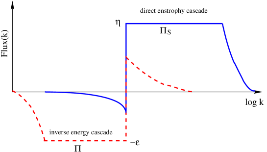
Figure 1: Cartoon depicting 2D turbulence theory: kinetic energy spectrum ($E(k)$, top panel) and fluxes (bottom panel) of enstrophy ($\Pi_{S}(k)$, blue solid line) and energy ($\Pi(k)$, red dashed line). Kinetic energy undergoes an inverse cascade to large scales (negative flux) at the kinetic energy injection rate, $\varepsilon$. Enstrophy undergoes a direct cascade to small scales at the enstrophy injection rate, $\eta$.

A general overview of 2D turbulence theory (see, e.g., [32]) is presented in Fig. 1. Kinetic energy, $|\mathbf{u}|^{2}/2$, and hence enstrophy, $|\zeta|^{2}/2$, are injected into the fluid. Because both are quadratic ideal invariants (conserved in the absence of forcing and viscosity) and $\zeta=\hat{\mathbf{z}}\cdot\nabla\times\mathbf{u}$, enstrophy cascades to smaller scales and energy undergoes an inverse cascade to larger scales (Fjortoft’s theorem). (The central point in deriving Fjortoft’s theorem is to realize that energy, $E(k)$, and enstrophy, $Z(k)$, spectra are related by $k^{2}E(k)=Z(k)$.) Under the assumption of spectral locality, forcing and dissipation cannot affect the flow except over a finite range of scales near where they are prescribed: far from these ranges, both cascades must therefore have a constant flux (Fig. 1, lower panel). The constant flux cascade regimes are called inertial ranges because only the inertial terms, $\mathbf{u}\cdot\nabla\mathbf{u}$ for energy and $\mathbf{u}\cdot\nabla\zeta=\{\psi,\zeta\}$ for enstrophy, are non-negligible. Dimensional analysis after equating constant fluxes to the inertial terms for energy and enstrophy yields a $k^{-5/3}$ energy spectrum in the inverse energy cascade and a $k^{-3}$ energy spectrum in the enstrophy cascade (Fig. 1, upper panel). Fine theoretical details such as the logarithmic correction to the $k^{-3}$ spectrum [29] and arguments about locality [33] have here been omitted.

2.2 Transfer analysis

The $\{\psi,\zeta\}$ term is the only non-negligible term in the enstrophy cascade regime. It will also be shown in Section 2.3 to be the term whose small-scale interactions we need to parameterize. It is thus the focus of our comparison methodology. Other terms in the analysis will heretofore be abbreviated as $\mathcal{F}$ for forcing, $\mathcal{D}$ for dissipation, and $\mathcal{Q}$ for large-scale drag (where, e.g., $\mathcal{F}\equiv\zeta F$). The time evolution of enstrophy at any physical position is given by the enstrophy-balance equation,

$$\partial_{t}\frac{1}{2}\zeta^{2}=\zeta\partial_{t}\zeta=-\zeta\{\psi,\zeta\}+\mathcal{F}+\mathcal{D}+\mathcal{Q}\,.$$ (2)

The time evolution of the enstrophy spectrum at wavenumber $k$, $Z(k)$, is similarly,

$$\partial_{t}Z(k)=\hat{\zeta}^{\ast}\partial_{t}\hat{\zeta}=S(k)+\mathcal{F}(k)+\mathcal{D}(k)+\mathcal{Q}(k)\,,$$ (3)

where $S(k)$ is the enstrophy transfer function (i.e., net enstrophy received by wavenumber $k$ from all other wavenumbers),

$$S(k)=-\hat{\zeta}^{\ast}(k)\widehat{\{\psi,\zeta\}}(k)\,,$$ (4)

and where the Fourier transform is represented by $\hat{\cdot}$ and complex-conjugation by $\cdot^{\ast}$. The flux of enstrophy through wavenumber $k$, i.e., the sum of the rate of change of enstrophy leaving all wavenumbers $\leq k$ and going to wavenumbers $>k$ (i.e., moving to smaller scales), is given by

$$\Pi_{S}(k)=-\int_{0}^{k}S(k^{\prime})dk^{\prime}\,,$$ (5)

that is, the total rate of enstrophy flowing past wavenumber $k$ to larger wavenumbers. The divergence of the flux is the transfer, $S(k)$. Because of the relation between energy and enstrophy spectra, the transfer of energy is $T(k)=S(k)/k^{2}$.

2.3 MOLES

To reduce computational cost, MOLES solve only the largest scales of a flow. The remaining unresolved scales from the anticipated higher-resolution simulation are filtered out. The filtering operation is indicated by $\bar{\cdot}$ and the resulting equations are

$$\partial_{t}\bar{\zeta}+\{\bar{\psi},\bar{\zeta}\}=\sigma+\bar{F}+\nu\nabla^{2}\bar{\zeta}-\overline{\frac{C_{D}}{h}{\hat{\mathbf{z}}\cdot}\nabla\times(|u|\mathbf{u})}\,,$$ (6)

where we have defined the subgrid term $\sigma\equiv-\overline{\{\psi,\zeta\}}+\{\bar{\psi},\bar{\zeta}\}$. The subgrid term is the effects on the resolved scales by unresolved fluid motions. How well it is modeled is the measure of the success of the MOLES. (Note that $\sigma={\hat{\mathbf{z}}\cdot}\nabla\times\nabla\cdot\tau$ where $\tau=-\overline{\mathbf{u}\mathbf{u}}+\bar{\mathbf{u}}\bar{\mathbf{u}}$, the momentum-equation LES subgrid stress tensor.) The time evolution of the enstrophy spectrum is now given by

$$\partial_{t}Z(k)=\bar{S}(k)+L(k)+{\mathcal{F}}(k)+\bar{\mathcal{D}}(k)+\mathcal{Q}(k)\,,$$ (7)

where $\bar{S}(k)$ is the rate of enstrophy received by wavenumber $k$ from all other resolved wavenumbers,

$$\bar{S}(k)=-\hat{\bar{\zeta}}^{\ast}\widehat{\{\bar{\psi},\bar{\zeta}\}}\,,$$ (8)

and $L(k)$ is the rate of enstrophy received from all unresolved wavenumbers,

$$L(k)=\hat{\bar{\zeta}}^{\ast}\hat{\sigma}\,.$$ (9)

Note that the rate of energy received from unresolved wavenumbers is $L(k)/k^{2}$. How closely the sum of enstrophy transfer functions, from resolved and unresolved wavenumbers, approximate the enstrophy transfer function from a fully resolved system,

$$\bar{S}(k)+L(k)\approx S(k)\,,$$ (10)

(for all wavenumbers smaller than the filter wavenumber) is the spectral measure of the success of the model. For $k$ in the inertial range, $S(k)=0$ and a successful model will produce $L(k)\approx-\bar{S}(k)$. The flux of enstrophy through wavenumber $k$ due to resolved and modeled interactions is given by

$$\Pi_{T}(k)=-\int_{0}^{k}{\big{[}}\bar{S}(k^{\prime})+L(k^{\prime}){\big{]}}dk^{\prime}\,.$$ (11)

2.4 Objective method: error-landscape of enstrophy flux

To objectively compare parameterizations, we make use of the error-landscape assessment [34, 35, 36, 37] on the enstrophy flux. We modify the method of [37] and employ $L^{1}$ instead of $L^{2}$ error norms,

$$D_{p}=\frac{\int_{1}^{k_{max}}\big{|}\Pi_{S}(k)-\Pi_{T}(k)\big{|}k^{p}dk}{\int_{1}^{k_{max}}\big{|}\Pi_{S}(k)\big{|}k^{p}dk}\,,$$ (12)

where $k_{max}$ is determined from the MOLES resolution (see below). We chose $p=0$ to obtain a good balance between the smaller resolved scales and the largest, less model-sensitive, scales. The optimal parameter value for each method is the point where this error norm is minimized. (The term landscape is intuitive for two-parameter models.) Inter-model comparisons are also made using the $D_{0}$ norm.

2.5 Design of numerical experiments

We employ a well-tested parallelized pseudo-spectral code [31]. The computational box has size $[2\pi]^{2}$, and wave numbers vary from $k_{min}=1$ to $k_{max}=N/3$ using a standard 2/3 de-aliasing rule, where $N$ is the number of grid points per direction. To cast our results in meaningful units, the results are dimensionalized by $l=l_{0}l^{\prime}$, $t=t_{0}t^{\prime}$ where $\cdot^{\prime}$ indicates non-dimensionalized pseudo-spectral result and $l_{0}=504\times 10^{4}/\pi\,$m and $t_{0}=1.2\times 10^{6}$s. To spin up our runs we begin with a $1008^{2}$ simulation (dimensionalized grid spacing $\Delta x=10\,$km) initialized with a few large-scale Fourier modes. The forcing is designed to mimic wind-stress at $k=4$:

$$F=A(t)\bigg{[}\cos{(4y+\phi_{y})}-\cos{(4x+\phi_{x})}\bigg{]}\,,$$ (13)

where $\phi_{x}=\pi\sin(1.2\times 10^{-6}\,$s${}^{-1}t)$ and $\phi_{y}=\pi\sin(1.2\times 10^{-6}\pi\,$s${}^{-1}t/3)$ so that the wind varies with a period of about 60 days. The coefficient $A$ is dynamically controlled to hold a steady enstrophy injection rate of $1.75\times 10^{-18}\,$s^-3 to reduce the amount of required statistics to measure a constant flux cascade, i.e.,

$$\frac{\int\zeta FdA}{\int dA}=1.75\times 10^{-18}\,s^{-3}\,.$$ (14)

Time step is $600\,$s, $\nu=88\,$m²s^-1, and $C_{D}/h=1.25\times 10^{-8}\,$m^-1. The resulting root-mean-squared velocity is $v_{rms}=2.6\,$ms^-1 and the forcing scale ($k=4$) is $L_{F}=2520\,$km. The corresponding forcing-scale turnover time is $11\,$days and the Reynolds number is $Re\equiv v_{rms}L_{F}/\nu\approx 75,000$. Simulations are integrated for over $1300\,$days. The final turbulent state of this run is used as initial conditions for the benchmark and MOLES runs at $\nu=1.375\,$m²s^-1.

3 Analysis of parameterizations

The goal of MOLES is to anticipate higher resolution results at an affordable resolution by representing the effects of the unresolved eddies. To avoid any bias between the parameterizations, we use as the benchmark a fully resolved direct numerical solution (DNS) at a resolution of $8192^{2}$ of a flow with $\nu=1.375\,$m²s^-1. Each MOLES is then run at a resolution of $1008^{2}$ and tested for its ability to reproduce the benchmark. This allows us to test the models’ representations against a known solution: a DNS flow. Accordingly, the MOLES simulations also must use $\nu=1.375\,$m²s^-1 in addition to the subgrid term or they should be compared, instead, to a $\nu=0$ benchmark which cannot be produced.

The benchmark is run for 390 days, $v_{rms}=2.6\,$ms^-1 and the corresponding forcing-scale turnover time is $11\,$days. The Reynolds number is $\approx 4.8\times 10^{6}$. A snapshot of the vorticity of the benchmark run is shown in the Upper Left panel of Fig. 2. There are several large vortices of both signs. Over time, vortices stretch and fold vortex filaments into the fine-scale features as seen. This is the enstrophy cascade process. This simulation is completely resolved and this cascade is arrested at the smallest scales by dissipation (Upper Right panel in Fig. 2). Energy is injected by the forcing term (Lower Right panel in Fig. 2) at a constant injection rate: an inverse cascade of energy and direct cascade of enstrophy result. The quadratic drag term serves to arrest the inverse cascade of kinetic energy and primarily removes energy (and enstrophy) at the largest scales. Though, it does remove both from a wide range of scales (Lower Left panel in Fig. 2).

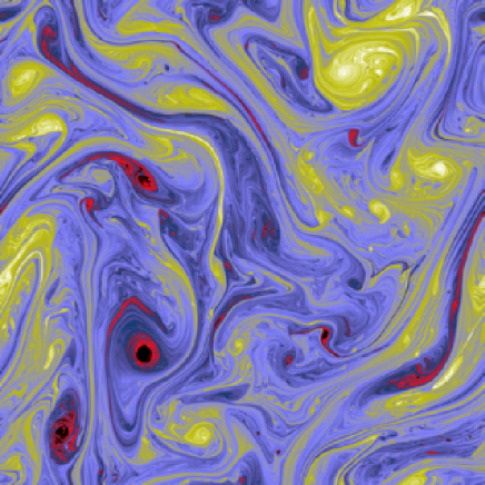
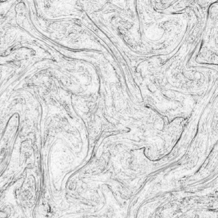
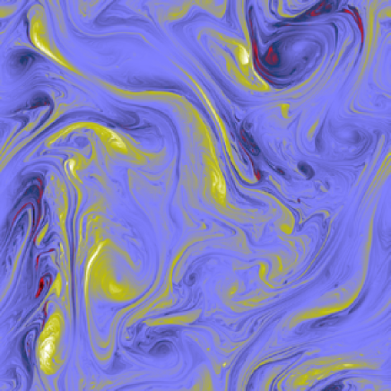
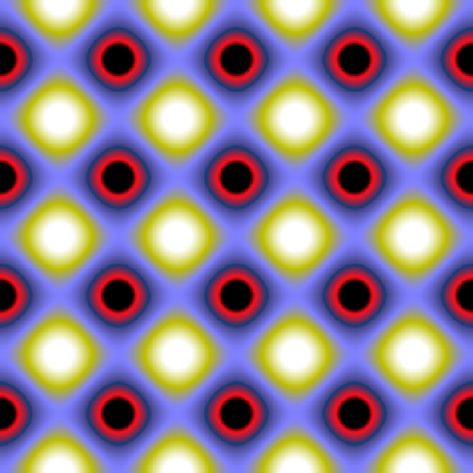
Figure 2: $8192^{2}$ benchmark; snapshot at 390 days for (Upper Left) vorticity, $\zeta$, with thresholds $\pm 1.5\times 10^{-5}\,$s^-1 (counter-clockwise vorticity is shown in yellow; clockwise in red); (Upper Right) absolute value of vorticity tendency due to dissipation, $\nu\nabla^{2}\zeta$, black pixels are $2.25\times 10^{-7}\,$s^-2; (Lower Left) vorticity tendency due to quadratic drag, $-\frac{C_{D}}{h}\nabla\times(|u|\mathbf{u})$, with thresholds $\pm 1.38\times 10^{-6}\,$s^-2; (Lower Right) vorticity tendency due to forcing, $F$, with thresholds $\pm 1\times 10^{-4}\,$s^-2.

The flux and resulting enstrophy spectrum for the benchmark are shown in Fig. 3. A power-law spectrum, $Z(k)\sim k^{-1.2}$, is observed in the enstrophy cascade inertial range. It is steeper than the predicted $k^{-1}$ spectrum due to the quadratic drag which acts at all scales of the flow: the difference between the enstrophy flux (solid line) and a constant flux is exactly the cumulative drag (dotted line). This steeper spectrum is similar to the result for linear drag [38]. Note that dissipation is not significant for wavenumbers, $k<300$. Reproducing this flow at a resolution of $1008^{2}$ ($k_{max}=336$) will thus be a onerous test for the parameterizations.

Figure 3: Benchmark run: (Top) Enstrophy flux ($\Pi_{S}(k)$, solid) and cumulative enstrophy injection (dash-triple-dotted), dissipation (dashed), and quadratic drag (dotted). As quadratic drag operates at all but the dissipative scales, a constant enstrophy flux range is not seen. (Bottom) Compensated enstrophy spectrum, $kZ(k)$, versus wavenumber, $k$, for $8192^{2}$ BVE benchmark. Quadratic drag acts at all scales and precludes a pure $Z(k)\sim k^{-1}$ spectrum.

The benchmark run contains all scales of motion at this $Re$. It can be used to calculate the true transfers with scales that will be unresolved at MOLES resolution by spectral cut-off filtering the benchmark run down to a resolution of $1008^{2}$. These subgrid transfers for energy and enstrophy are plotted in Fig. 4. The effects of the subgrid scales are to remove enstrophy from a narrow band of wavenumbers near the resolution limit and to generate a small amount of energy at the very largest scales. These transfers can also been seen in Fig. 7 of [9]. The upscale energy transfer is a strong function of the resolution, $\Delta x$: as can be seen by comparison with [9], the smaller $\Delta x$ is, the smaller in magnitude is the upscale energy transfer. In fact, in the limit as $\Delta x$ approaches $\nu^{1/2}$ times some constant, both subgrid transfers will tend to zero [28]. However, at fixed $\Delta x$ both transfers will tend to a non-zero function of $k$ that remains the same in the limit of zero viscosity. This is due to spectral locality: only those scales nearest $\Delta x$ will contribute to the transfers. As $\nu$ decreases, and more and more scales are added, they will contribute less and less to the transfers for $k<1/\Delta x$.

Given that an ideal MOLES will have $L(k)$ that exactly reproduces Fig. 4, we can anticipate the performance of the proposed closures. None of the purely dissipative models (viscous, hyper-viscous, Leith, or Smagorinsky) will be able to reproduce the upscale transfer of energy. The hyper-viscous model should better confine enstrophy dissipation to large wave numbers as its subgrid term contains fourth-order derivatives compared to second-order for the viscous model and first-order derivatives of the product of first-order derivatives for Leith. Smagorinsky is derived for 3D flow and is not expected to perform well in 2D. It has been previously shown that AVM can produce the correct forms of the transfers if high enough order viscosities and small enough anticipation times are employed [9]. The $\alpha-$model is non-dissipative, but could potentially transport energy in the correct direction [27].

Figure 4: Benchmark run: Transfers with what will be unresolved scales for MOLES simulations for enstrophy, $S(k)-\bar{S}(k)$ (solid line), and energy, $[S(k)-\bar{S}(k)]/k^{2}$ (dashed line). An ideal MOLES would exactly reproduce these transfers with $L(k)=S(k)-\bar{S}(k)$.

3.1 Linear viscous parameterizations and their performance

The simplest parameterization is to assume the main effect of subgrid turbulence is dissipative. Accordingly, the viscosity is often increased until a numerically resolved solution is possible. The subgrid term, $\sigma$, in the MOLES equation, Eq. (6) is then

$$\sigma=\big{(}\nu^{\prime}-\nu\big{)}\nabla^{2}\zeta\,,$$ (15)

with $\nu^{\prime}\gg\nu$. A slightly more sophisticated approach is to add higher-order dissipation, hyper-viscosity, e.g.

$$\sigma=\nu_{4}\nabla^{4}\zeta\,,$$ (16)

or even higher order. We focus on $\nabla^{2}$ and $\nabla^{4}$ parameterizations here.

We apply the error-landscape of enstrophy flux technique to optimize the viscous model. The modeled flux, $\Pi_{T}(k)$, for the viscous model is shown in Fig. 5. Note that as the viscosity is varied, the modeled flux brackets both sides of the benchmark flux. This suggests an optimal $\nu^{\prime}$ for the model should be indicated by the enstrophy flux error-landscape. Indeed, $D_{0}$ has its minimum for ${\nu^{\prime}}=11\,$m²s^-1. This is the optimal viscous model which we will compare to the other parameterizations.

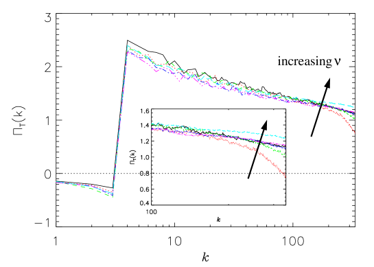
Figure 5: Viscous model: (Top) Modeled flux, $\Pi_{T}(k)$, for ${\nu^{\prime}}=5.5\,$m²s^-1 (red dotted), $11\,$m²s^-1 (green dashed), $16.5\,$m²s^-1 (blue dash-dotted), $22\,$m²s^-1 (pink dash-triple-dotted), and $24.75\,$m²s^-1 (cyan long-dashed) and $\Pi_{S}(k)$ for $8192^{2}$ BVE benchmark (solid black). (Bottom) Flux error-landscape norm $D_{0}$. The optimal value is ${\nu^{\prime}}=11\,$m²s^-1.

The approximate reproduction of the benchmark flux is accomplished by the action of the subgrid enstrophy transfer $L(k)$ (Fig. 6). As expected, the action of the viscous model is solely dissipative. The solid black line indicates what the true transfer with the unresolved scales should be, $S(k)-\bar{S}(k)$ (see Fig. 4). The viscous model dissipates enstrophy over a much larger range of scales. Moreover, since energy is dissipated as $\sim\nu^{\prime}Z(k)\sim k^{-1.2}$, eddy viscosity is unphysically positive at large scales. What the unresolved scales should be doing is contributing to the upscale transfer of energy as shown by the solid, black benchmark line. The enstrophy spectra are shown in Fig. 7. The result of too little dissipation is the piling of small-scale thermal noise in the spectrum [39].

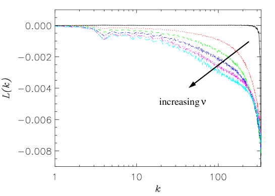
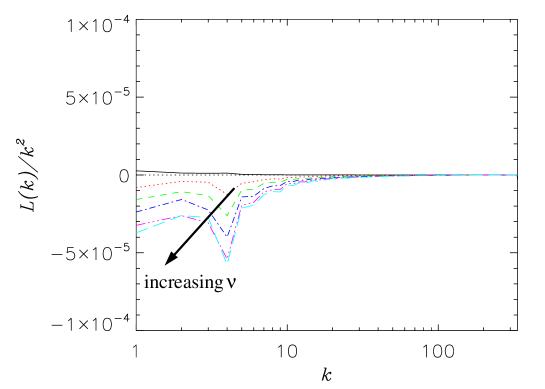
Figure 6: Viscous model: subgrid transfers for enstrophy ($L(k)$, Top) and energy ($L(k)/k^{2}$, Bottom) and $S(k)-\bar{S}(k)$ for benchmark (solid black). The model is solely dissipative of enstrophy and energy. Exact viscosities are denoted in Fig. 5.

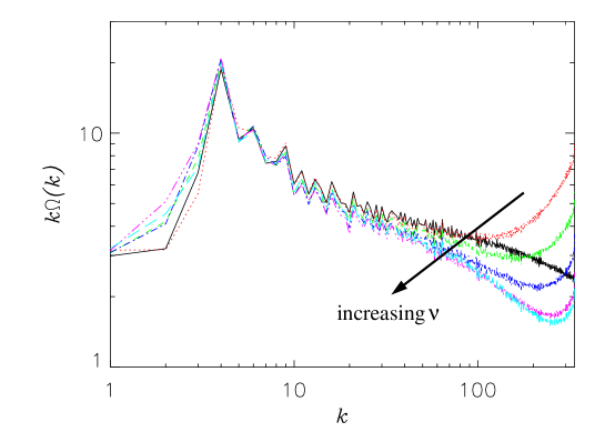
Figure 7: Viscous model: Compensated enstrophy spectrum; exact viscosities are denoted in Fig. 5.

By looking at the hyper-viscous model’s flux error-landscape norms (Fig. 8), we identify $\nu_{4}=1.1\times 10^{9}\,$m⁴s^-1 as the optimal hyper-viscous model. The hyper-viscous model much more closely models the dissipation of enstrophy due to the unresolved scales than the viscous model, see Fig. 9. Additionally, as the energy dissipation is $\sim k^{2}Z\sim k^{0.8}$, the rate of energy dissipated at large scales is insignificant (note the difference in vertical scales for energy transfer in Figs. 4, 6 and 9). This is a marked improvement, but no solely-dissipative parameterization will model the mechanism of upscale energy transfer.

Figure 8: Hyper-viscous model: Flux error-landscape norm $D_{0}$. The optimal value is $\nu_{4}=1.1\times 10^{9}\,$m⁴s^-1.

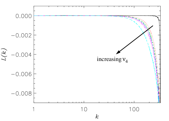
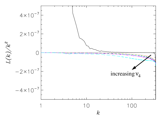
Figure 9: Hyper-viscous model: Subgrid transfers for enstrophy ($L(k)$, Top) and energy ($L(k)/k^{2}$, Bottom) for $\nu_{4}=2.2\times 10^{8}\,$m⁴s^-1 (red dotted), $3.3\times 10^{8}\,$m⁴s^-1 (green dashed), $4.4\times 10^{8}\,$m⁴s^-1 (blue dash-dotted), $5.5\times 10^{8}\,$m⁴s^-1 (pink dash-triple-dotted), $1.1\times 10^{9}\,$m⁴s^-1 (cyan long-dashed), and $S(k)-\bar{S}(k)$ for benchmark (solid black).

3.2 Leith model

The Leith model is derived by dimensional analysis [4]. The local enstrophy dissipation rate is estimated as

$$\eta_{\ast}=\nu_{\ast}\big{|}\nabla_{\ast}\bar{\zeta}\big{|}^{2}\,,$$ (17)

and an enstrophy cascade spectrum is assumed,

$$Z(k)\propto\eta^{2/3}k^{-1}\,.$$ (18)

The viscous range, $k$, is when the viscous enstrophy losses in a given wavenumber band, $\int\nu k^{2}Z(k)dk$, are comparable to the enstrophy injection, $\eta$, or

$$\eta\sim\nu^{3}k^{6}\,.$$ (19)

Setting the global average dissipation, $\nu$, to the local, grid-scale dissipation rate, $\nu_{\ast}$, and equating Eqs. (17) and (19), we find

$$\nu_{\ast}\propto\big{|}\nabla\bar{\zeta}\big{|}(\Delta x)^{3}\,.$$ (20)

The BVE with Leith model, is [4, 1]

$$\partial_{t}\bar{\zeta}+\{\bar{\psi},\bar{\zeta}\}=\nabla\cdot\nu\nabla\bar{\zeta}+\nabla\cdot\nu_{\ast}\nabla\bar{\zeta}{+\bar{F}+\bar{Q}}\,,$$ (21)

where $\nu=0$ for an infinite Reynolds number flow. The Leith subgrid term is then

$$\sigma=\nabla\cdot\bigg{[}\bigg{(}\frac{\Lambda\Delta x}{\pi}\bigg{)}^{3}\big{|}\nabla\bar{\zeta}\big{|}\nabla\bar{\zeta}\bigg{]}\,,$$ (22)

where $\Lambda$ is a free parameter.

The subgrid transfers for the Leith model are very similar to the viscous model results (see Fig. 10). This is to be expected as the Leith model is also solely-dissipative. Note that there is strong enstrophy dissipation at the forcing scale. This can be understood by looking at Fig. 11. The Leith viscosity $\nu_{\ast}$ is proportional to $|\nabla\bar{\zeta}|$ and, therefore, is concentrated along the borders between oppositely-signed vortices. These large-scale coherent structures of enhanced dissipation then project on the small wavenumber Fourier-modes (bottom left panel of Fig. 11). Note that the optimal parameter value is found to be $\Lambda=1$.

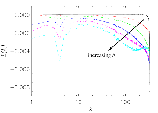
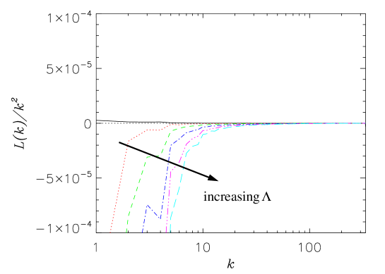
Figure 10: Leith model: Subgrid transfers for enstrophy ($L(k)$, Top) and energy ($L(k)/k^{2}$, Bottom) for $\Lambda=0.5$ (red dotted), $\Lambda=0.75$ (green dashed), $\Lambda=1$ (blue dash-dotted), $\Lambda=1.25$ (pink dash-triple-dotted), $\Lambda=1.5$ (cyan long-dashed), and benchmark (black solid). The optimal model is $\Lambda=1$.

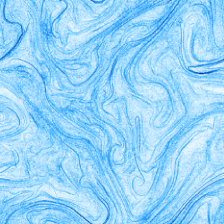
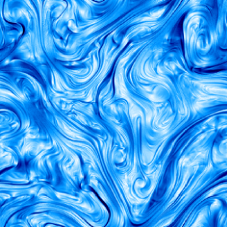
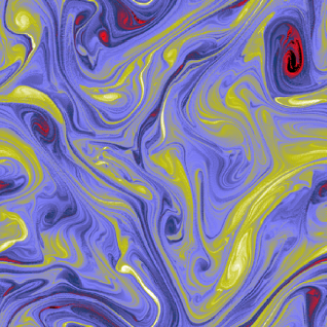
Figure 11: Snapshots of $\nu_{\ast}$ (Top Left) and Fourier power spectrum of $\nu_{\ast}$ (Bottom Left) for Leith model, $\Lambda=1$, of $\nu_{\ast}$ (Top Right) for Smagorinsky, $\Lambda_{S}=1$, and of vorticity field (Bottom Right, shown for reference). All snapshots are at $4\times 10^{4}\,$min.

3.3 Smagorinsky model

The Smagorinsky model [3, 40] is the 3D precursor of the Leith model. It is derived with a similar dimensional analysis as in Sec. 3.2, but assuming a 3D direct cascade of energy. Consequently, the model for eddy-viscosity is

$$\nu_{\ast}=\bigg{(}\frac{{\Lambda_{S}}\Delta x}{\pi}\bigg{)}^{2}|S_{ij}|\,,$$ (23)

where $S_{ij}=(\partial_{j}v_{i}+\partial_{i}v_{j})/2$. For isotropic, homogeneous 3D turbulence the Smagorinsky Constant, $C_{S}\equiv{\Lambda_{S}}/\pi\approx 0.2$ [41]. It should be noted that Smagorinsky was devised for 3D isotropic flow and was not intended for 2D nor geostrophic flows, but has been employed in global climate models [42, 43].

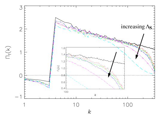
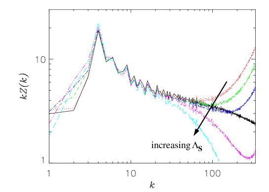
Figure 12: Smagorinsky model: (Top) Modeled flux, $\Pi_{T}(k)$, for $\Lambda_{S}=0.1$ (red dotted), $\Lambda_{S}=0.3$ (green dashed), $\Lambda_{S}=0.5$ (blue dash-dotted), $\Lambda_{S}=1$ (pink dash-triple-dotted), and $\Lambda_{S}=2$ (cyan long-dashed) and $\Pi_{S}(k)$ for $8192^{2}$ BVE benchmark (solid black). (Bottom) Compensated enstrophy spectrum.

The enstrophy flux and enstrophy spectrum for Smagorinsky (Fig. 12), highlight the fact that good spectra can be produced without necessarily reproducing the correct dynamics. The best spectra are produced for $\Lambda_{S}=0.5$ (blue dash-dotted) while the best flux is produced by $\Lambda_{S}=0.1$ (red dotted). This is opposed to the case for the viscous model where the best flux and spectrum occur for the same value of the model’s one free parameter, $\nu^{\prime}$. The reason for the disparity is that the viscous parameterization captures the most important physical process, small-scale enstrophy dissipation, while the Smagorinsky model unphysically removes enstrophy and energy from the largest scales (see Fig. 13 and the real-space visualization of $\nu_{\ast}$ in Fig. 11). Therefore, even when the combination of modeling and numerical error produces a good spectrum, the model is not capturing the correct physical dynamics.

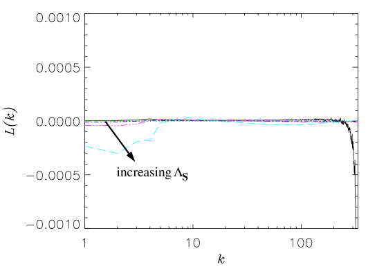
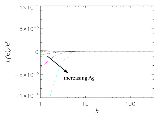
Figure 13: Smagorinsky model: subgrid transfers of enstrophy ($L(k)$, Top) and energy ($L(k)/k^{2}$, Bottom). The model dissipates enstrophy and energy unphysically from the large scales. Exact viscosities are denoted in Fig. 12.

3.4 Anticipated vorticity method (AVM)

AVM (APVM when applied to potential vorticity, [8]) is so-called because it can be seen as substituting the forward-in-time vorticity in the BVE,

$$\frac{\bar{\zeta}_{n+1}-\bar{\zeta}_{n}}{\theta}=-\{\bar{\psi},\bar{\zeta}_{n}\}\,,$$ (24)

where $\theta$ is the time step for the anticipation. Substituting this anticipated value, $\bar{\zeta}_{n+1}$ in Eq. (1) results in the lowest-order AVM,

$$\partial_{t}\bar{\zeta}=-\{\bar{\psi},\bar{\zeta}_{n}\}+\theta\{\bar{\psi},\{\bar{\psi},\bar{\zeta}_{n}\}\}{+\bar{F}+\bar{D}+\bar{Q}}\,.$$ (25)

In practice, to weight the subgrid model to smaller scales,

$$\sigma=-\frac{\theta}{k_{max}^{2m}}\{\bar{\psi},\nabla^{2m}\{\bar{\psi},\bar{\zeta}\}\}\,,$$ (26)

In this study we have used $m=1$ as even this order of diffusive operator is not practical in finite-volume and finite-difference schemes typically used in global ocean modeling because of the relationship between high-order derivative accuracy and stencil size. AVM is not Galilean invariant, i.e., it does not conserve momentum, but it exactly conserves energy while dissipating enstrophy. Note that the subgrid term for the momentum equation is $\nabla\cdot\tau=\big{[}(-1)^{m}\frac{\theta}{k_{max}^{2m}}\nabla^{2m}\big{(}\mathbf{u}\cdot\nabla(\zeta\hat{\mathbf{z}}\times\mathbf{u})\big{)}\big{]}\hat{\mathbf{z}}\times\mathbf{u}$ which is perpendicular to the velocity at every point in space. AVM then exactly conserves energy even if $\theta$ varies spatially and temporally.

As AVM dissipates enstrophy at small scales, $L(k)<0$ for large $k$ (see Fig. 14), it must also remove some small-scale energy, $k^{-2}L(k)<0$. Since AVM exactly conserves energy, this energy shows up at large scales. AVM is the only parameterization studied here that reproduces this signature of the correct transfer. The physical effect, however, is over estimated by at least an order of magnitude. This can be mitigated by reducing $\theta$. However, too small $\theta$ (0.125$dt$ for our flow) results in an excess of energy at all scales [9]. For $m=1$, as used here, AVM is unable to mimic that eddy viscosity should only act in a small range of wavenumbers near $k_{max}$ [9]. Note that setting the anticipation time equal to the time step, $\theta=1$, very closely reproduces the low-wavenumber flux (Fig. 15). This large value for $\theta$, however, makes the eddy viscosity act at even larger scales (Fig. 14). If larger values of $m$ were practical in actual ocean applications, a two parameter optimization might yield a very robust model. Holding constant $m=1$, the optimal value of $\theta$ is $0.16$.

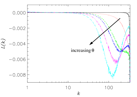
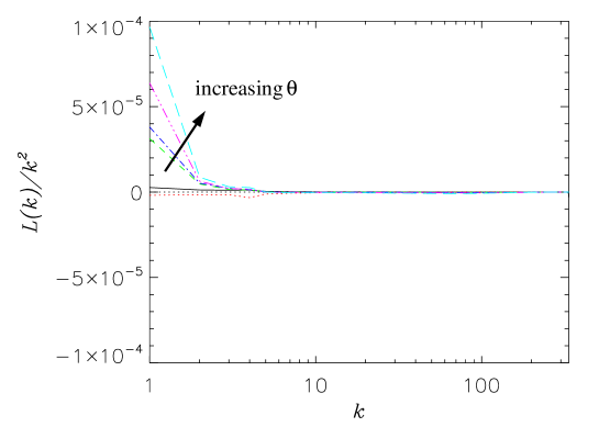
Figure 14: AVM: Subgrid transfers of enstrophy ($L(k)$, Top) and energy ($L(k)/k^{2}$, Bottom) for $8192^{2}$ BVE benchmark (solid black), for $\theta=0$ (NO MODEL, red dotted), $\theta=0.16$ (green dashed), $0.25$ (blue dash-dotted), $0.5$ (pink dash-triple-dotted), and $1$ (cyan long-dashed). The subgrid model transfer in AVM changes sign so that the model dissipates no energy, sum of $L(k)/k^{2}$ over all wavenumbers is $o(10^{-12})$, while enstrophy dissipation (sum of $L(k)$) is $o(1)$. The negative energy dissipation at large scales mimics the upscale transfer from unresolved scales, though too strongly.

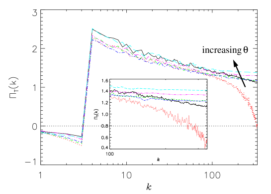
Figure 15: AVM: (Top) Modeled flux, $\Pi_{T}(k)$. Exact values of $\theta$ are given in Fig. 14. (Bottom) Flux error-landscape norm. Optimal value is $\theta=0.16$.

3.5 $\alpha-$model

The $\alpha-$model takes a different approach than the other parameterizations. It is a non-dissipative, solely dispersive model – a mathematical regularization (smooth, and hence computable solutions are ensured even in the limit $\nu\rightarrow 0$) of the fluid equations [12, 13, 14, 15, 16, 17]. The result is that the vorticity is advected by a smoothed velocity, $\overline{\mathbf{u_{s}}}=(1-\alpha^{2}\nabla^{2})^{-1}\bar{\mathbf{u}}$, with a filter scale $\sim\alpha$,

$$\partial_{t}\bar{\zeta}+\nabla\cdot\bigg{(}\overline{\mathbf{u_{s}}}\bar{\zeta}\bigg{)}=\nu\nabla^{2}\bar{\zeta}+{\bar{F}+\bar{D}+\bar{Q}}\,,$$ (27)

where $\nabla\cdot\bigg{(}\overline{\mathbf{u_{s}}}\bar{\zeta}\bigg{)}=\{\bar{\psi_{s}},\bar{\zeta}\}$. The alpha subgrid term is

$$\sigma=\{\bar{\psi},\bar{\zeta}\}-\{\bar{\psi_{s}},\bar{\zeta}\}\,.$$ (28)

Note that the $\alpha-$model has complex conservation properties in that the energy balance equation is in the $H^{1}_{\alpha}$ norm, $\int\overline{\mathbf{u_{s}}}\cdot\bar{\mathbf{u}}dA$, and enstrophy is in the $L^{2}$ norm, $\int\bar{\zeta}^{2}dA$. The subgrid energy transfer is $L_{\alpha}(k)/k^{2}$ is related to the subgrid enstrophy transfer by $L_{\alpha}(k)=L(k)/(1+\alpha^{2}k^{2})$.

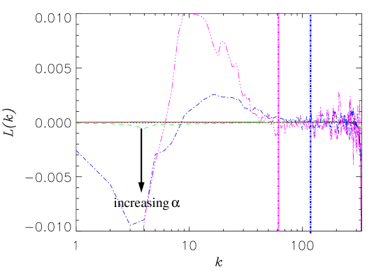
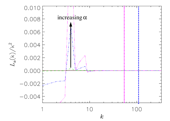
Figure 16: $\alpha-$model: subgrid transfers of enstrophy ($L(k)$, Top) and energy ($L_{\alpha}(k)/k^{2}$, Bottom) for $\alpha=\Delta x$ (red dotted), $2\Delta x$ (green dashed), $9\Delta x$ (blue dash-dotted; vertical line shows wavenumber), $16\Delta x$ (pink dash-triple-dotted; vertical line shows wavenumber), and benchmark (solid black, nearly zero except for $k\gtrapprox 300$ in $L(k)$). Due to numerical cancellation noise in Eq. (28), smoothing has been applied to the plots.

The subgrid transfers, Fig. 16, for the $\alpha-$model are very large and in the wrong direction. As the model dissipates neither energy nor enstrophy the transfers are conservative; they remove energy and enstrophy from above the forcing scale and deposit them below the forcing scale. As the filter width, $\alpha$, is increased so is the amount of large-scale energy and enstrophy moved down-scale to scales larger than $\alpha$ (vertical lines in Fig. 16).

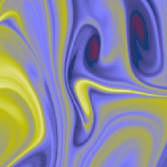
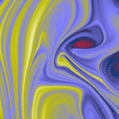
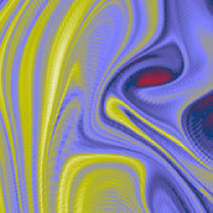
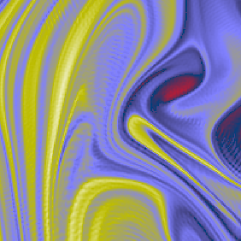
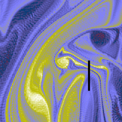
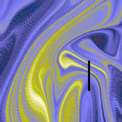
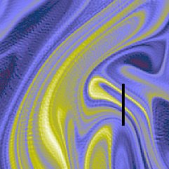
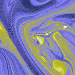
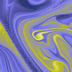
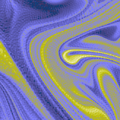
Figure 17: Vorticity field, $\zeta$: Vortex merger event (tracked to center of field of view which is $1/5^{2}$ of the entire domain). Time runs from top to bottom starting 0min after initialization in steps of $10^{4}\,$min. 1st column LANS $\alpha=2\Delta x$, 2nd column $9\Delta x$, 3rd column $16\Delta x$. $\alpha=2\Delta x$ is the most realistic result. Cuts from 3rd row (black lines) are plotted in Fig. 18.

The physical effects of the $\alpha-$model are visualized in Fig. 17: small-scale vortical motions are removed from the advecting field. As $\alpha$ is increased the rotation of the central, yellow(light) V-shaped, vorticity feature is reduced. This can be seen by viewing each row from left to right. To visualize the effect on the vorticity filaments, 1D cuts are taken as indicated by the black lines in the third row. The vorticity values are plotted in Fig. 18. There is a translation due to the removal of small-scale vorticity from the advecting field. Disregarding this, it is seen that the filaments are slightly larger as $\alpha$ is increased. The vorticity peaks are also taller. This indicates that the dissipation of the filaments is reduced as $\alpha$ is increased. The effect is also seen in the spectra: enstrophy is removed from the largest (and smallest) scales and deposited at scales bracketed by the forcing scale and $\alpha$. One interpretation could be that the $\alpha-$model reduces both the roll-up and the thinning of filamentation. The reduced roll-up reduces spatially averaged vorticity gradients and, hence, reduces dissipation. The reduction in thinning of the filaments does not appear to be large enough to be significant for the dissipation of individual, small filaments. Also due to this, more vorticity and enstrophy remains at super$-\alpha$ scales.

Note that our $\alpha-$model spectra do not compare to results found by [27]: their forcing kept $Z_{s}(10)$ constant rather than enstrophy injection constant, dissipated based on $\zeta_{s}$ not $\zeta$, and plotted different quantities than we have here. They studied $|u_{s}|^{2}$ and $|\zeta_{s}|^{2}$ which are not the ideal invariants for the $\alpha-$model. Finally, unlike for the 3D $\alpha-$model [17], no change in the scaling of the dissipation scale with Reynolds number is expected for the 2D $\alpha-$model [28]. This suggests 2D$-\alpha$ will not perform as a LES in the same regard as its 3D counterpart and, perhaps, explains our results.

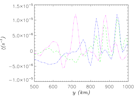
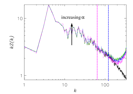
Figure 18: $\alpha-$model: (Top) Cut of vorticity field, $2\times 10^{4}\,$min into simulation for $\alpha=2\Delta x$ (green dashed), $9\Delta x$ (blue dash-dotted), and $16\Delta x$ (pink dash-triple-dotted). Section of cut is indicated in 3rd row of Fig. 17. (Bottom) Compensated enstrophy spectrum for same time.

3.6 Comparison of parameterizations

The subgrid transfers of the six parameterizations are compared in Fig. 19. Concentrating on the subgrid enstrophy transfer, we can eliminate the $\alpha-$model because it unphysically generates enstrophy for $100\lessapprox k\lessapprox 200$ and Smagorinsky can be eliminated because it essentially eliminates zero small-scale enstrophy (the grey line is flat an indistinguishable from zero on this vertical scale). Of the remaining models, the hyper-viscous is closest to mimicking the true subgrid transfers of both energy and enstrophy, though for the largest wavenumbers, $k>200$, the viscous and Leith parameterizations perform similarly. The AVM is the only method that reproduces the correct sign of the energy transfer, but it removes enstrophy preferentially from intermediate scales instead of the smallest resolved scales. This method would likely perform better for $m>1$ [9].

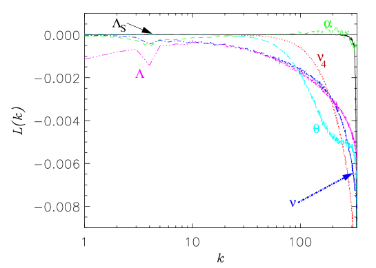
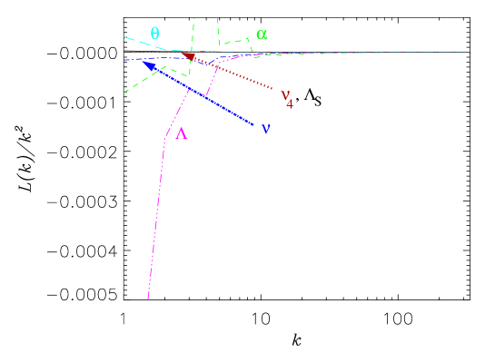
Figure 19: Subgrid transfers of enstrophy ($L(k)$, Top) and energy ($L(k)/k^{2}$, Bottom) for benchmark (solid black), hyper-viscous $\nu_{4}=1.1\times 10^{-9}m^{4}s^{-1}$ (red dotted), LANS $\alpha=2\Delta x$ (green dashed), viscous $\nu=11m^{2}s^{-1}$ (blue dash-dotted), Leith $\Lambda=1$ (pink dash-triple-dotted), AVM $\theta=0.16$ (cyan long-dashed), and Smagorinsky $\Lambda_{S}=0.1$ (solid grey).

The enstrophy flux error landscape norms are given in Fig. 20. The $\alpha-$model and Smagorinsky are the obvious outliers with a factor of five poorer performance. The viscous, hyper-viscous and Leith parameterizations have very similar performance. The AVM is within a factor of two in performance. Again, this could likely be improved upon by using a larger value of $m$.

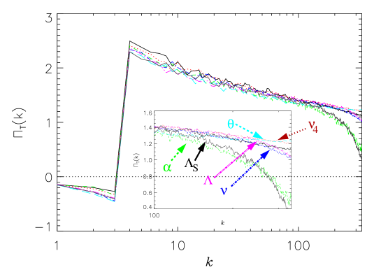
Figure 20: (Top) Enstrophy flux error-landscape norm $D_{0}$ for hyper-viscous ($\nu_{4}$), $\alpha-$model ($\alpha$), $\nabla^{2}$ viscosity ($\nu$), Leith ($\Lambda$), AVM ($\theta$), and Smagorinsky ($\Lambda_{S}$). (Bottom) Modeled enstrophy flux, $\Pi_{T}$, for for benchmark (solid black), hyper-viscous $\nu_{4}=1.1\times 10^{-9}m^{4}s^{-1}$ (red dotted), LANS $\alpha=2\Delta x$ (green dashed), viscous $\nu=11m^{2}s^{-1}$ (blue dash-dotted), Leith $\Lambda=1$ (pink dash-triple-dotted), AVM $\theta=0.16$ (cyan long-dashed), and Smagorinsky $\Lambda_{S}=0.1$ (solid grey).

This similarity in performance between hyper-viscous, viscous, and Leith parameterizations can also been seen in the resulting enstrophy spectra, Fig. 21. All three methods have the same spectra for $k\lessapprox 100$. Neither the $\alpha-$model nor Smagorinsky reduces the pile-up of numerical thermalization noise [39] in the small scales. As seen in the previous results, the AVM method with $m=1$ is dissipative at too large scales to perform as well as the viscous, hyper-viscous, or Leith parameterizations. Smagorinsky performs poorly because it removes enstrophy from the largest rather than the smallest resolved scales.

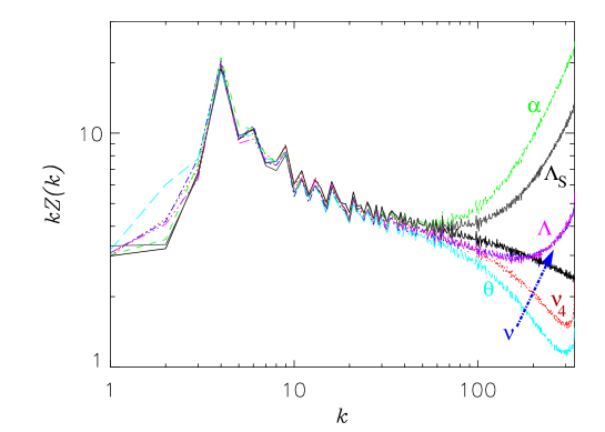
Figure 21: Enstrophy spectra for benchmark (solid black), hyper-viscous $\nu_{4}=1.1\times 10^{-9}m^{4}s^{-1}$ (red dotted), LANS $\alpha=2\Delta x$ (green dashed), viscous ${\nu^{\prime}}=11m^{2}s^{-1}$ (blue dash-dotted), Leith $\Lambda=1$ (pink dash-triple-dotted), AVM $\theta=0.16$ (cyan long-dashed), and Smagorinsky $\Lambda_{S}=0.1$ (solid grey).

4 Conclusions

We have compared six popular turbulence parameterizations in the enstrophy cascade regime of the barotropic vorticity equation on a $f-$plane (equivalently, 2D Navier-Stokes) in forced-dissipative simulations. The hyper-viscous, viscous, and Leith models all perform well down to about $10\Delta x$. The hyper-viscous model reproduces the largest-resolved-scales ($1\leq k\leq 100$) flux the best of the three and the viscous model best reproduces the smallest-resolved-scales ($k\geq 200$) flux. The Leith model, because its diffusion is anisotropic, is expected to carry-over its performance to anisotropic flows (e.g., the 3D baroclinic ocean system) which would be challenging for the viscous and hyper-viscous models. The Smagorinsky model does not work in the enstrophy cascade regime–it removes enstrophy from the largest rather than the smallest resolved scales. The anticipated vorticity method without a strong enough weighting to small scales, larger values of $m$, does not perform as well as the prior three parameterizations. As even this order of diffusive operator is not practical in the finite-volume and finite-difference schemes typically used in global ocean modeling (e.g., [44]), we chose not to investigate higher-orders.

We have confirmed [28]’s suggestion that the Lagrangian-averaged $\alpha-$model does not perform as a turbulence model in this system (see also [27]). Analytically, one expects the numerical degrees of freedom to scale with Reynolds number the same as unparameterized Navier-Stokes. The model reduces rotation due to small-scale vorticity and, less dramatically, also reduces the thinning of vortex filaments due to stretching. The balance of the effect is a net reduction of dissipation of the vorticity filaments and a piling of energy and enstrophy to sub-forcing/super$-\alpha$ scales (enhancing the flux in this spectral region).

One possible MOLES closure has not been scoped here, the use of monotone transport as the model for LES closure. These closures, commonly referred to Monotone Implicit Large-Eddy Simulation (MILES), require the evaluation of the nonlinear transport be carried out in physical space, something that is not possible within the global spectral model utilized for this study. Our future work, discussed briefly below, will utilize a traditional finite-volume approach where an evaluation of MILES will be possible. Combined models have also not been investigated here due to the enormous parameter space that would entail.

Subgrid transfers have been measured before, e.g., for the APVM [9], and again for the APVM, hyper-viscosity, and implicit large-eddy simulations [45]. Error-landscapes for LES have been produced for various quantities like spectra [34, 35, 36, 37]. By combining these two techniques, however, we have introduced a method for determining the optimal turbulence parameterization also in flows different than those considered here: the error-landscape of the enstrophy flux at small-scales in a 2D flow can be replaced by the error-landscape of the modeled flux in a 3D baroclinic system (see A). We emphasize that MOLES comparisons based on spectra alone do not ensure that the correct dynamics are being reproduced by a parameterization. For example, consider the $\Lambda_{S}=0.5$ ($C_{S}\approx 0.16$) result for the Smagorinsky model (blue dash-dotted line in Fig. 12). The spectrum is best approximated by this run, but for the wrong reasons as the non-linear flux is more poorly reproduced than for $\Lambda_{S}=0.1$. For the viscous model, however, which physically correctly removes enstrophy from the small scales, both the spectrum and the flux are best reproduced for ${\nu^{\prime}}=11\,$m²s^-1. In this latter case, the spectrum is reproduced because the dynamics are reproduced.

For a 3D baroclinic system, at the scales on which the MOLES acts ($5-10\,$km), the system will be approximately QG. Because of the similarities between QG and 2D [1], we have some expectation that our results will hold: Smagorinsky, the $\alpha-$model, and APVM with $m=1$ will not perform as well as viscosity, hyper-viscosity, and Leith. In fact, because of the anisotropic diffusion offered by Leith, it will likely perform the best. Our results may not extend to the 3D system, however, if additional physics comes in to play, like vertical mixing over small horizontal scales.

Our next step is to move into an idealized, 3D baroclinic system, most likely a re-entrant zonal channel that can serve as an idealized Antarctic Circumpolar Current. While the move to three dimensions allows for the direct simulation of baroclinic instability, it also necessitates the development of analysis tools that can accurately account for energy and enstrophy transfers between the disparate horizontal and vertical scales of motion. Furthermore, the move to a 3D baroclinic system entails the use of a height-based vertical coordinate. Such a system requires the transport of one or more tracers in order to close the system via an equation of state. The theoretical analysis of such a system is outlined in A. And finally, as we move to more realistic and, thus, bounded domains, our ability to simulate the governing equations, as well as analyze the fluxes, via global spectral expansions will be increasingly cumbersome. As a result, we plan on utilizing a traditional finite-volume global ocean model [46] in the next phase of this study.

Acknowledgments We acknowledge discussions with B. Fox Kemper, D. Holm, and B. Wingate. This work was supported by the Earth System Modeling and Regional and Global Climate Modeling programs of the Office of Biological and Environmental Research within the US Department of Energy’s Office of Science.

Appendix A 3D baroclinic case

In this section, we apply our methodology to a 3D baroclinic system of equations. The hydrostatic, traditionally shallow, and simple Boussinesq equations, e.g., as solved by [46], are

$$\frac{\partial{\bf u}}{\partial t}+\frac{1}{2}\nabla_{h}\left|{\bf u}\right|^{2}+(f+\zeta)\hat{\mathbf{z}}\times\mathbf{u}+w\frac{\partial{\bf u}}{\partial z}=-\frac{1}{\rho_{0}}\nabla_{h}p+F+D+Q$$ (29)

$$\nabla_{3}\cdot\mathbf{v}=0$$ (30)

$$\partial_{t}\rho+\nabla_{h}(\rho\mathbf{u})+\partial_{z}(\rho w)=0$$ (31)

$$\partial_{t}(\rho T)+\nabla_{h}(\rho T\mathbf{u})+\partial_{z}(\rho Tw)=0$$ (32)

where $\mathbf{v}=\mathbf{u}+w\hat{\mathbf{z}}$ is the full 3D velocity field, $\mathbf{u}$ and $w$ are the horizontal and vertical components, $\nabla_{h}$ is the 2D horizontal gradient, $\nabla_{3}$ is the full 3D gradient, $f$ is the Coriolis force, $\zeta=\hat{\mathbf{z}}\cdot\nabla_{h}\times\mathbf{u}$ is the vertical component of vorticity, $\rho_{0}$ is the background density, $p$ is the pressure, and $T$ is the temperature. We have assumed constant salinity and a linear equation of state for simplicity.

Unlike for the 2D case, for the 3D system, we must also consider transfer between available potential (APE) and kinetic energies. The time evolution of the horizontal kinetic energy, $KE\equiv\mathbf{u}^{2}/2$, is given by

$$\partial_{t}(KE)+{\nabla_{3}\cdot\big{[}\mathbf{v}(KE+\frac{p}{\rho_{0}})\big{]}}={-\frac{g\rho}{\rho_{0}}w}$$ (33)

Where we make use of the hydrostatic condition, $\partial_{z}{p}=-g{\rho}$, and have left off the terms $\mathbf{u}\cdot\mathbf{F}+\mathbf{u}\cdot\mathbf{D}+\mathbf{u}\cdot\mathbf{Q}$ for brevity. We define the APE, $\Phi$, implicitly by $\big{(}\partial_{z}\Phi\big{)}_{\rho T}\equiv{g\rho}/{\rho_{0}}$. From this, we can derive [32]

$$\frac{D\Phi}{Dt}=\bigg{(}\frac{D\Phi}{D\rho T}\bigg{)}_{z}\frac{D\rho T}{Dt}+\bigg{(}\frac{D\Phi}{Dz}\bigg{)}_{\rho T}\frac{Dz}{Dt}=\frac{g\rho}{\rho_{0}}w$$

$$\partial_{t}\Phi+{\nabla_{3}\cdot(\Phi\mathbf{v})}={\frac{g\rho}{\rho_{0}}w}$$ (34)

The sum of horizontal kinetic energy and available potential energy is ideally conserved (i.e., when $F=D=Q=0$ and no transport occurs across the system boundaries). The exchange between the two energy reservoirs is via the $g\rho w/\rho_{0}$ term.

The transfer functions for the 3D ocean system determine the time rate of change of the horizontal kinetic energy “spectrum,”

$$\partial_{t}KE_{\kappa}=TKK_{\kappa}+TKKP_{\kappa}+TAK_{\kappa}\,,$$ (35)

where $\mathcal{B}{\{}\cdot\}_{\kappa}$ will represent projection onto a complete orthonormal basis. For example, in a zonally-reentrant channel this basis could be Fourier modes in the zonal direction, sines in the meridional direction, and baroclinic eigenmodes in the vertical. The transfer of $KE$ from other modes to a given orthonormal mode (equivalent of $T(k)=S(k)/k^{2}$) is

$$TKK_{\kappa}=-\mathcal{B}{\{}\mathbf{u}{\}}_{\kappa}^{\ast}\cdot\mathcal{B}\bigg{\{}\mathbf{v}\cdot\nabla_{3}\mathbf{u}\bigg{\}}_{\kappa}$$ (36)

where $\mathbf{v}\cdot\nabla_{3}\mathbf{u}=\nabla_{h}KE+\zeta\hat{\mathbf{z}}\times\mathbf{u}+w\partial_{z}{\bf u}$, the transfer of $KE$ from other modes due to the pressure term is

$$TKKP_{\kappa}=-\mathcal{B}\big{\{}\mathbf{v}\big{\}}_{\kappa}^{\ast}\cdot\mathcal{B}\bigg{\{}\nabla_{3}\frac{p}{\rho_{0}}\bigg{\}}_{\kappa}\,,$$ (37)

and net transfer rate from APE to $KE_{\kappa}$ is

$$TAK_{\kappa}=-\mathcal{B}\big{\{}w\big{\}}_{\kappa}^{\ast}\cdot\mathcal{B}\bigg{\{}\frac{g\rho}{\rho_{0}}\bigg{\}}_{\kappa}\,.$$ (38)

Similarly, expressions for the transfer functions for Eq. (34) can be written. As we have shown for the 2D case, the method to determine the best turbulence closure for an eddy-permitting ocean model is to compute the transfer functions derived here (and their integrals, the fluxes). Then, the $D_{0}$ norm error-landscape will be computed for each potential MOLES by comparison with a high resolution benchmark run.

References

- [1] B. Fox-Kemper, D. Menemenlis, Can large eddy simulation techniques improve mesoscale-rich ocean models?, in: M. Hecht, H. Hasumi (Eds.), Ocean Modeling in an Eddying Regime, Vol. 177, AGU Geophysical Monograph Series, 2008, pp. 319–338.
- [2] C. Meneveau, J. Katz, Scale-Invariance and Turbulence Models for Large-Eddy Simulation, Annual Review of Fluid Mechanics 32 (2000) 1–32.
- [3] J. Smagorinsky, General Circulation Experiments with the Primitive Equations, Monthly Weather Review 91 (1963) 99.
- [4] C. E. Leith, Stochastic models of chaotic systems, Physica D 98 (1996) 481–491.
- [5] M. Lesieur, O. Métais, P. Comte, Large-Eddy Simulations of Turbulence, 2005.
- [6] B. Fox-Kemper, J. Pedlosky, Wind-driven barotropic gyre I: Circulation control by eddy vorticity fluxes to an enhanced removal region, Journal of Marine Research 62 (2) (2004) 169–193.
- [7] B. Fox-Kemper, Reevaluating the roles of eddies in multiple barotropic wind-driven gyres, Journal of Physical Oceanography 35 (7) (2005) 1263–1278.
- [8] R. Sadourny, C. Basdevant, Parameterization of Subgrid Scale Barotropic and Baroclinic Eddies in Quasi-geostrophic Models: Anticipated Potential Vorticity Method., Journal of Atmospheric Sciences 42 (1985) 1353–1363.
- [9] G. K. Vallis, B.-L. Hua, Eddy viscosity of the anticipated potential vorticity method, Journal of Atmospheric Sciences 45 (1988) 617–627.
- [10] Q. Chen, M. Gunzburger, T. Ringler, A Scale-Invariant Formulation of the Anticipated Potential Vorticity Method, Monthly Weather Review 139 (2011) 2614–2629.
- [11] F. Gay-Balmaz, D. D. Holm, Parameterizing interaction of disparate scales: Selective decay by Casimir dissipation in fluids, ArXiv e-printsarXiv:1206.2607.
- [12] D. D. Holm, J. E. Marsden, T. S. Ratiu, Euler-Poincaré Models of Ideal Fluids with Nonlinear Dispersion, Physical Review Letters 80 (1998) 4173–4176.
- [13] S. Chen, C. Foias, D. D. Holm, E. Olson, E. S. Titi, S. Wynne, Camassa-Holm Equations as a Closure Model for Turbulent Channel and Pipe Flow, Physical Review Letters 81 (1998) 5338–5341.
- [14] S. Chen, C. Foias, D. D. Holm, E. Olson, E. S. Titi, S. Wynne, The Camassa-Holm equations and turbulence, Physica D Nonlinear Phenomena 133 (1999) 49–65.
- [15] S. Chen, D. D. Holm, L. G. Margolin, R. Zhang, Direct numerical simulations of the Navier-Stokes alpha model, Physica D Nonlinear Phenomena 133 (1999) 66–83.
- [16] S. Chen, C. Foias, D. D. Holm, E. Olson, E. S. Titi, S. Wynne, A connection between the Camassa-Holm equations and turbulent flows in channels and pipes, Physics of Fluids 11 (1999) 2343–2353.
- [17] C. Foias, D. D. Holm, E. S. Titi, The Navier-Stokes-alpha model of fluid turbulence, Physica D Nonlinear Phenomena 152 (2001) 505–519.
- [18] J. Pietarila Graham, D. D. Holm, P. D. Mininni, A. Pouquet, Highly turbulent solutions of the Lagrangian-averaged Navier-Stokes model and their large-eddy-simulation potential, Phys. Rev. E. 76 (5) (2007) 056310.
- [19] J. Pietarila Graham, P. D. Mininni, A. Pouquet, Lagrangian-averaged model for magnetohydrodynamic turbulence and the absence of bottlenecks, Phys. Rev. E 80 (1) (2009) 016313.
- [20] J. Pietarila Graham, P. D. Mininni, A. Pouquet, High Reynolds number magnetohydrodynamic turbulence using a Lagrangian model, Phys. Rev. E 84 (1) (2011) 016314.
- [21] B. T. Nadiga, L. G. Margolin, Dispersive Dissipative Eddy Parameterization in a Barotropic Model, Journal of Physical Oceanography 31 (2001) 2525–2531.
- [22] D. D. Holm, B. T. Nadiga, Modeling Mesoscale Turbulence in the Barotropic Double-Gyre Circulation, Journal of Physical Oceanography 33 (2003) 2355.
- [23] B. A. Wingate, The Maximum Allowable Time Step for the Shallow Water Model and Its Relation to Time-Implicit Differencing, Monthly Weather Review 132 (2004) 2719.
- [24] D. D. Holm, B. A. Wingate, Baroclinic Instabilities of the Two-Layer Quasigeostrophic Alpha Model, Journal of Physical Oceanography 35 (2005) 1287.
- [25] M. W. Hecht, D. D. Holm, M. R. Petersen, B. A. Wingate, Implementation of the LANS- turbulence model in a primitive equation ocean model, Journal of Computational Physics 227 (2008) 5691–5716.
- [26] M. W. Hecht, D. D. Holm, M. R. Petersen, B. A. Wingate, The LANS- and Leray turbulence parameterizations in primitive equation ocean modeling, Journal of Physics A Mathematical General 41 (2008) H4009.
- [27] B. T. Nadiga, S. Shkoller, Enhancement of the inverse-cascade of energy in the two-dimensional Lagrangian-averaged Navier-Stokes equations, Physics of Fluids 13 (2001) 1528–1531.
- [28] E. Lunasin, S. Kurien, M. A. Taylor, E. S. Titi, A study of the Navier-Stokes- model for two-dimensional turbulence, Journal of Turbulence 8 (2007) 30.
- [29] R. H. Kraichnan, Inertial-range transfer in two- and three-dimensional turbulence, Journal of Fluid Mechanics 47 (1971) 525–535.
- [30] M. E. Maltrud, G. K. Vallis, Energy and enstrophy transfer in numerical simulations of two-dimensional turbulence, Physics of Fluids 5 (1993) 1760–1775.
- [31] P. D. Mininni, D. L. Rosenberg, R. Reddy, A. Pouquet, An hybrid MPI-OpenMP scheme for scalable parallel pseudospectral computations for fluid turbulence, Parallel Computing 37 (2011) 316.
- [32] G. K. Vallis, Atmospheric and Oceanic Fluid Dynamics, 2006.
- [33] Z. Xiao, M. Wan, S. Chen, G. L. Eyink, Physical mechanism of the inverse energy cascade of two-dimensional turbulence: a numerical investigation, Journal of Fluid Mechanics 619 (2008) 1.
- [34] J. Meyers, B. J. Geurts, M. Baelmans, Database analysis of errors in large-eddy simulation, Physics of Fluids 15 (2003) 2740–2755.
- [35] J. Meyers, P. Sagaut, B. J. Geurts, Optimal model parameters for multi-objective large-eddy simulations, Physics of Fluids 18 (9) (2006) 095103.
- [36] J. Meyers, B. J. Geurts, P. Sagaut, A computational error-assessment of central finite-volume discretizations in large-eddy simulation using a Smagorinsky model, Journal of Computational Physics 227 (2007) 156–173.
- [37] J. Meyers, Error-landscape assessment of large-eddy simulations: a review of the methodology, J. Sci. Comp. 49 (2011) 65–77.
- [38] S. Danilov, D. Gurarie, Nonuniversal features of forced two-dimensional turbulence in the energy range, Phys. Rev. E 63 (2) (2001) 020203.
- [39] C. Cichowlas, P. Bonaïti, F. Debbasch, M. Brachet, Effective Dissipation and Turbulence in Spectrally Truncated Euler Flows, Physical Review Letters 95 (26) (2005) 264502.
- [40] D. K. Lilly, The representation of small-scale turbulence in numerical simulation experiments, in: Proc. IBM Scientific Computing Symp. Environ. Sci., 1967, p. 195.
- [41] C. Meneveau, J. Katz, Scale-Invariance and Turbulence Models for Large-Eddy Simulation, Annual Review of Fluid Mechanics 32 (2000) 1–32.
- [42] S. M. Griffies, R. W. Hallberg, Biharmonic Friction with a Smagorinsky-Like Viscosity for Use in Large-Scale Eddy-Permitting Ocean Models, Monthly Weather Review 128 (2000) 2935.
- [43] T. L. Delworth, A. Rosati, W. Anderson, A. J. Adcroft, V. Balaji, R. Benson, K. Dixon, S. M. Griffies, H.-C. Lee, R. C. Pacanowski, G. A. Vecchi, A. T. Wittenberg, F. Zeng, R. Zhang, Simulated Climate and Climate Change in the GFDL CM2.5 High-Resolution Coupled Climate Model, Journal of Climate 25 (2012) 2755–2781.
- [44] T. D. Ringler, J. Thuburn, J. B. Klemp, W. C. Skamarock, A unified approach to energy conservation and potential vorticity dynamics for arbitrarily-structured C-grids, Journal of Computational Physics 229 (2010) 3065–3090.
- [45] J. Thuburn, J. Kent, N. Wood (Eds.), Energy and Enstrophy Cascades in Numerical Models, 2011.
- [46] T. D. Ringler, M. R. Petersen, D. Jacobsen, R. L. Higdon, P. W. Jones, M. E. Maltrud, A Multi-Resolution Approach to Global Ocean Modeling, Ocean Modeling, under revision.