Fundamental properties of the Population II fiducial stars HD 122563 and Gmb 1830 from CHARA interferometric observations

We have determined the angular diameters of two metal-poor stars, HD 122563 and Gmb 1830, using CHARA and Palomar Testbed Interferometer observations. For the giant star HD 122563, we derive an angular diameter $\theta_{\rm 3D}=0.940\pm 0.011$ milliarcseconds (mas) using limb-darkening from 3D convection simulations and for the dwarf star Gmb 1830 (HD 103095) we obtain a 1D limb-darkened angular diameter $\theta_{\rm 1D}=0.679\pm 0.007$ mas. Coupling the angular diameters with photometry yields effective temperatures with precisions better than 55 K ($T_{\rm eff}$ = 4598 $\pm$ 41 K and 4818 $\pm$ 54 K — for the giant and the dwarf star, respectively). Including their distances results in very well-determined luminosities and radii ($L=230\pm 6$ L_⊙, $R=23.9\pm 1.9$ R_⊙ and $L=0.213\pm 0.002$ L_⊙, $R=0.664\pm 0.015$ R_⊙, respectively). We used the CESAM2k stellar structure and evolution code in order to produce models that fit the observational data. We found values of the mixing-length parameter $\alpha$ (which describes 1D convection) that depend on the mass of the star. The masses were determined from the models with precisions of $<$3% and with the well-measured radii excellent constraints on the surface gravity are obtained ($\log g=1.60\pm 0.04,4.59\pm 0.02$ dex, respectively). The very small errors on both $\log g$ and $T_{\rm eff}$ provide stringent constraints for spectroscopic analyses given the sensitivity of abundances to both of these values. The precise determination of $T_{\rm eff}$ for the two stars brings into question the photometric scales for metal-poor stars.

1 Introduction

Metal-poor stars are some of the oldest stars in the Galaxy and thus reflect the chemical composition of Galactic matter at the early stages of Galactic evolution. The determination of accurate observed fundamental properties, and in particular their location in the Hertzsprung-Russell (HR) diagram, is a key requirement if we aim to constrain the unobservable properties such as mass, age, and initial helium content by using stellar models. Among the most controversial observed parameter is the effective temperature ($T_{\rm eff}$) which can vary by more than 200 K for metal-poor stars from one method to another (see the PASTEL catalogue, Soubiran et al. 2010). In particular, local thermodynamic equilibrium (LTE) is usually assumed and non-LTE (NLTE) effects must be included in spectroscopic analyses especially for metal-poor stars where these effects are enhanced (Thévenin & Idiart 1999; Andrievsky et al. 2010; Merle et al. 2011) and this leads to even more discrepancy between literature values. One solution is to measure the angular diameter and convert this to $T_{\rm eff}$ to provide a direct determination.

The large majority of metal-poor stars belong to the halo or the old disk of the Galaxy which means that their apparent magnitude and or angular diameters are extremely small and difficult to measure. However, some instruments, in particular those on the CHARA array (ten Brummelaar et al. 2005) are very capable of working at short wavelengths on long baselines to obtain the required angular resolution. Among the most exciting possible targets with CHARA working in the $K$ band are HD 122563 (= HR 5270, HIP 68594, m_V = 6.19 mag) and Gmb 1830 (= HD 103095, LHS 44, HIP 57939, m_V = 6.45 mag) whose mean metallicities $[Z/X]_{s}$ are $\sim$–2.3 dex and –1.3 dex, respectively (see discussion in Sect. 4.1), where $Z$ and $X$ denote the metallicity and hydrogen (absolute) mass fraction in the star and the subscript refers to the observed surface value.

HD 122563, a standard example of a very metal-poor field giant (Wallerstein et al. 1963; Wolffram 1972), has been extensively studied and presents similarities with metal-poor giants found in globular clusters. Gmb 1830 is a metal-poor halo dwarf star recognized as exhibiting depleted Li (Deliyannis et al. 1994; King 1997) when compared to the mean value of halo dwarf stars (Spite & Spite 1993; Ryan 2005). It is also the nearest halo dwarf and has an excellent parallax measurement. Combining interferometric measurements of these stars with other already measured old moderately metal-poor stars, such as $\mu$ Cas ([$Z/X$]_s = -0.5 dex, Boyajian et al. 2008), offers an excellent opportunity to constrain the $T_{\rm eff}$ scale of metal-poor stars over a wide range of metallicities with possible implications for $T_{\rm eff}$ calibrations of globular cluster stars. In Table 1 we summarize some of the most recent determinations of the atmospheric properties of both targets. Note that HD 122563 and Gmb 1830 have also been defined as benchmark stars for the Gaia mission under the SAM working group.

Not only are temperature scales for metal-poor stars controversial, but stellar structure and evolution models often predict higher $T_{\rm eff}$ than those observed for these stars (see e.g. Fig. 2 of Lebreton 2000). The difficulty encountered when trying to match evolutionary tracks to the observational data not only severely inhibits the determination of any fundamental properties but any chance of improving or testing the physics in the models is also limited.

Considering the difficulties mentioned above, in this paper we aim to determine accurate fundamental properties of HD 122563 and Gmb 1830 based on interferometric observations (Sect. 2). In Sect. 3 we present our analysis of the observations to determine the angular diameters of both stars. We then determine the observed values of $T_{\rm eff}$, luminosity $L$, and radius $R$, and subsequently use stellar models to constrain the unobservable properties of mass $M$, initial metal and helium content $Z_{\rm{}_{i}},Y_{\rm i}$, mixing-length parameter $\alpha$ and age (Sect. 4). We also predict their global asteroseismic properties in order to determine if such observations could further constrain the models.

Table 1: Most recent photometric and spectroscopic determinations of atmospheric parameters for the target stars

HD 122563				Gmb 1830
$T_{\rm eff}$	$\log g$	[Fe/H]	p/sa	$T_{\rm eff}$	$\log g$	[Fe/H]	p/s
(K)	(dex)	(dex)		(K)	(dex)	(dex)
$4795^{b}$			p	5129b			p
4598c			p	5011c			p
4572d			p	5054e			p
4600f	1.50	-2.53	s	5250g	5.00	-1.26	s
4570h	1.10	-2.42	s	5070i	4.69	-1.35	s

Notes. ^ap/s = photometric/spectroscopic determination. ^bGonzález Hernández & Bonifacio (2009) ^cRamírez & Meléndez (2005) ^dAlonso et al. (1999a) ^eBlackwell & Lynas-Gray (1998) ^fNLTE analysis by Mashonkina et al. (2008) ^gLuck & Heiter (2006) ^hMishenina & Kovtyukh (2001) ⁱGehren et al. (2006)

2 Observations

The observations were collected at the CHARA Array (ten Brummelaar et al. 2005), located at Mount Wilson Observatory (California), together with two beam combining instruments: CHARA Classic and FLUOR. CHARA Classic (ten Brummelaar et al. 2005) is a two-telescope, pupil-plane, open-air beam combiner working in both the $H$ and $K^{\prime}$ bands, and our observations correspond to the $K^{\prime}$ band (the central wavelength is $\lambda=2.141\,\mu$m, from Bowsher et al. 2010). The raw data were reduced using the pipeline described in ten Brummelaar et al. (2005). FLUOR (Coudé du Foresto et al. 1998; Mérand et al. 2006) is a two-telescope beam combiner, but uses single-mode optical fibers for recombination. Single-mode fibers efficiently reduce the perturbations induced by the turbulent atmosphere on the stellar light wavefront, as the injected light corresponds only to the mode guided by the fiber (Ruilier 1999; Coudé du Foresto 1998). Most of the atmospherically corrupted part of the wavefront is lost into the cladding, and the beam combination therefore occurs between two almost coherent beams. This results in an improved stability of the measured fringe contrast. The FLUOR data reduction pipeline (Mérand et al. 2006, see also Kervella et al. 2004b) is based on the Fourier algorithm and was developed by Coudé du Foresto et al. (1997).

Table 2: CHARA observations of HD 122563 and Gmb 1830.

MJD	Inst.	$B$	PA	$V$	$\sigma(V)$
(days)		(m)	(∘)
HD 122563
54603.427	F	294.07	-18.4	0.599	0.015
54602.329	F	284.90	8.3	0.648	0.015
54602.309	F	288.89	13.7	0.630	0.014
54579.797	C	312.54	240.4	0.562	0.067
54579.784	C	316.88	238.2	0.617	0.064
54579.772	C	320.35	236.5	0.534	0.063
54579.760	C	323.52	235.0	0.554	0.071
54579.748	C	326.10	233.6	0.543	0.101
54578.812	C	308.35	242.5	0.587	0.059
54578.801	C	312.18	240.6	0.529	0.064
54578.786	C	316.86	238.2	0.483	0.057
54578.771	C	321.19	236.1	0.498	0.072
54578.755	C	325.23	234.1	0.469	0.057
54645.698	C	287.58	257.8	0.606	0.074
54645.686	C	290.38	254.8	0.584	0.080
54645.676	C	292.87	252.6	0.509	0.086
54645.670	C	294.78	251.1	0.527	0.075
Gmb 1830
54604.314	F	330.49	-11.5	0.744	0.023
54604.279	F	330.16	-3.3	0.751	0.022
54604.241	F	330.23	5.7	0.756	0.022
54459.022	C	327.54	238.9	0.696	0.053
54459.013	C	326.45	237.4	0.724	0.047
54459.005	C	325.16	235.9	0.691	0.051
54458.996	C	323.67	234.4	0.733	0.031
54458.959	C	313.47	228.3	0.714	0.053
54458.950	C	310.34	227.1	0.734	0.055
54458.935	C	304.08	225.0	0.759	0.043
54458.927	C	299.91	223.9	0.757	0.036
54421.060	C	312.48	227.9	0.752	0.073
54421.053	C	310.12	227.0	0.756	0.064
54421.047	C	307.47	226.1	0.755	0.057
54421.040	C	304.69	225.2	0.759	0.064
54421.032	C	300.68	224.1	0.769	0.066
54421.018	C	293.59	222.4	0.776	0.056
54421.009	C	288.24	221.3	0.773	0.090

We observed HD 122563 and Gmb 1830 in late 2007 and 2008 with FLUOR and Classic. The corresponding visibility measurements $V$ and uncertainties $\sigma(V)$ are listed in Table 2 along with the projected baseline $B$ and the baseline position angle PA measured clockwise from North. To monitor the interferometric transfer function, we interspersed the observations of our two science targets with calibrator stars. The calibrators for the FLUOR observations were selected from the catalogue by Mérand et al. (2005), and these are listed in Table 3, and those for the CHARA Classic observations used the calibrators presented in Table 4.

Table 3: FLUOR calibrator stars.

Calibrator	Sp. type	$m_{\mathrm{V}}$	$m_{\mathrm{K}}$	UD (mas)	Target
HD 129336	G8III	5.6	3.4	$0.98\pm 0.01$	HD 122563
HD 127227	K5III	7.5	4.0	$0.84\pm 0.01$	HD 122563
HD 108123	K0III	6.0	3.7	$0.93\pm 0.01$	Gmb 1830
HD 106184	K5III	7.7	3.5	$0.98\pm 0.01$	Gmb 1830

Table 4: CHARA Classic calibrator Stars

Calibrator	Sp. type	$m_{\mathrm{V}}$	$m_{\mathrm{K}}$	UD (mas)	Target
HD 119550	G2V	6.9	5.3	$0.389\pm 0.027$	HD 122563
HD 120066	G0V	6.3	4.9	$0.479\pm 0.033$	HD 122563
HD 120934	A1V	6.1	6.0	$0.198\pm 0.014$	HD 122563
HD 121560	F6V	6.2	4.8	$0.460\pm 0.030$	HD 122563
HD 122365	A2V	6.0	5.7	$0.238\pm 0.016$	HD 122563
HD 103799	F6V	6.6	5.3	$0.343\pm 0.013$	Gmb 1830

We also retrieved archival observations of HD 122563 in the $K$ band obtained with the Palomar Testbed Interferometer (PTI) (Colavita et al. 1999) between 1999 and 2002, and these are listed in Table 5. The data processing algorithm that was employed to reduce the PTI observations has been described in detail by Colavita (1999). Due to the shorter baselines, the PTI observations resolve HD 122563 marginally, and therefore do not strongly constrain its angular diameter. However, thanks to the relatively large number of observations, they provide an independent method for testing any bias in the CHARA observations.

3 From visibilities to limb-darkened angular diameters

We employed a non-linear, least-squares fitting routine in IDL (MPFIT, Markwardt 2009) to fit uniform disk and limb-darkened visibility functions for a single star to the calibrated data points (see Hanbury Brown et al. 1974; Boyajian et al. 2012). We obtained a uniform disk diameter for HD 122563 and Gmb 1830 of $\theta_{\rm UD}=0.924\pm 0.011$ mas and $\theta_{\rm UD}=0.664\pm 0.015$ mas, respectively. We used the linear limb-darkening coefficients from Claret (2000) assuming a [Fe/H]$=-2.5$, $T_{\rm eff}=4500$ K, and $\log g=1.0$ for HD 122563 and [Fe/H]$=-1.5$, $T_{\rm eff}=5000$ K, and $\log g=4.5$ for Gmb 1830. The assumptions on these parameters on the adopted coefficients have minimal influence on the final limb-darkened diameter, adding uncertainties of only a few tenths of a percent, well within the errors of our diameter measurements. We obtained $\theta_{\rm LD}=0.948\pm 0.012$ and $\theta_{\rm LD}=0.679\pm 0.015$ for HD 122563 and Gmb 1830, respectively.

We obtained a reduced $\chi^{2}$ value of 0.28 for HD 122563 and 0.18 for Gmb 1830 from the fits. These values, much less than 1, are indicative of our individual measurement errors being over estimated. We show the data and the visibility function fits for HD 122563 and Gmb 1830 in Figures 1 and 2. The results from the fits to the data yield 1D limb-darkened angular diameters of HD122563 and Gmb 1830 with a precision of $\sim$2% (see Table 6), respectively.

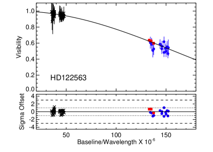
Figure 1: Calibrated observations for PTI (black crosses), CHARA Classic (blue circles) and CHARA FLUOR (red squares) data plotted with the 1D limb-darkened visibility function fit for HD 122563. See Section 3 for details.

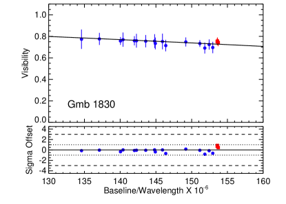
Figure 2: Calibrated observations for CHARA Classic (blue circles) and CHARA FLUOR (red squares) data plotted with the limb-darkened visibility function fit for Gmb 1830. See Section 3 for details.

Table 5: PTI observations of HD 122563.

MJD	$B$	$V$	$\sigma(V)$
(days)	(m)
51255.371	105.63	0.914	0.043
51255.384	104.32	0.940	0.030
52000.309	107.55	0.939	0.017
52000.320	106.67	0.947	0.015
52000.329	105.88	0.948	0.016
52000.334	105.37	0.948	0.018
52023.231	108.58	0.933	0.028
52023.271	105.38	0.957	0.048
52023.313	101.08	0.958	0.031
52041.196	107.66	0.974	0.080
52041.206	106.83	0.933	0.056
52041.229	104.73	0.957	0.035
52041.236	103.99	0.954	0.031
52041.258	101.62	0.908	0.043
52041.267	100.70	0.912	0.047
52044.236	103.14	0.910	0.046
52044.243	102.39	0.948	0.060
52044.276	99.00	0.959	0.061
52044.283	98.36	0.943	0.061
52306.520	102.86	0.973	0.072
52306.522	102.68	0.941	0.061
52306.535	101.36	0.963	0.066
52306.552	99.54	0.980	0.083
52306.554	99.37	0.969	0.074
52306.569	97.96	0.962	0.106
52328.424	84.82	0.981	0.035
52328.432	85.50	0.993	0.040
52328.450	86.41	0.968	0.047
52328.459	86.47	0.941	0.087
52329.419	84.57	0.965	0.056
52329.426	85.24	0.984	0.023
52329.438	86.08	0.973	0.022
52329.445	86.36	0.966	0.030
52329.464	86.33	0.986	0.019
52329.471	86.04	0.979	0.031
52329.490	84.51	0.938	0.030
52329.498	83.52	0.933	0.054
52329.516	80.61	0.960	0.052
52353.369	85.86	0.970	0.053
52353.385	86.46	0.988	0.056
52353.392	86.46	0.993	0.067
52353.426	84.27	0.975	0.105
52353.433	83.39	0.987	0.107
52353.451	80.54	0.989	0.119
52353.455	79.88	0.993	0.139
52359.378	86.42	0.929	0.093
52359.386	86.18	0.963	0.084
52359.423	82.58	0.904	0.191
52359.431	81.24	0.866	0.104

3.1 3D limb-darkened angular diameter for HD 122563

Convection plays a very important role in the determination of stellar limb-darkening. It has been shown that a 3D hydrodynamical treatment of the surface layers can lead to a significative change of temperature gradients compared to 1D hydrostatic modeling, which consequently affects the center-to-limb intensity variation (e.g. Allende Prieto et al. 2002; Bigot et al. 2006; Pereira et al. 2009; Chiavassa et al. 2010; Bigot et al. 2011; Hayek et al. 2012). The 3D/1D limb-darkening correction for a giant star can be very significant (see Fig. 6 of Chiavassa et al. 2010) and is generally much stronger than for a dwarf star. We therefore used a radiative-hydrodynamical (RHD) surface convection simulation of a red giant for HD 122563 to determine the 3D limb-darkened angular diameter. The parameters of the model are $\langle T_{\rm{eff}}\rangle=4627\pm 14$K (temporal average and standard deviation of the effective temperature), [Fe/H]=$-$3.0, and $\log g$ = 1.6 (Collet et al. 2009; Chiavassa et al. 2010). The computational domain of the RHD simulation represents only a small portion of the stellar surface ($\sim$1/30 of the circumspherence), however, it is sufficiently large to contain enough granules ($\sim$10-15) at each time step of the simulation. Hydrodynamical equations are solved on a staggered mesh with a conservative scheme. Details of the computation can be found in Collet et al. (2009).

Table 6: Angular diameters

	# of	$\theta_{\rm UD}\pm\sigma$	$\theta_{\rm 1D}\pm\sigma$	$\theta_{\rm 3D}\pm\sigma$
Star	Observations	(mas)	(mas)	(mas)
Gmb 1830	18	$0.664\pm 0.015$	$0.679\pm 0.015$
HD 122563	66	$0.924\pm 0.011$	$0.948\pm 0.012$	$0.940\pm 0.011$

We computed emergent intensity for a representative series of simulated snapshots and for wavelengths corresponding to the FLUOR filter ($2.14\pm 0.26$ $\mu$m, equivalent to that for CHARA) using the 3D pure-LTE radiative transfer code Optim3D (Chiavassa et al. 2009). It considers the Doppler shifts due to convective motions. Radiative transfer is solved monochromatically using pre-tabulated extinction coefficients for the same chemical compositions as the RHD simulations. It also uses the same extensive atomic and molecular opacity data as the latest generation of MARCS models (Gustafsson et al. 2008).

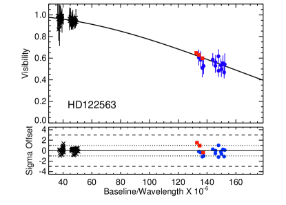
Figure 3: Best matching 3D-RHD synthetic visibility curves and PTI (black crosses), Classic (blue circles), and FLUOR (red squares) data for HD 122563.

For each time-step, we solve the radiative transfer equation for different inclinations with respect to the vertical whose cosines are $\mu{\equiv}$[1.000, 0.989, 0.978, 0.946, 0.913, 0.861, 0.809, 0.739, 0.669, 0.584, 0.500, 0.404, 0.309, 0.206, 0.104]. From these limb-darkened intensities, we derived the monochromatic visibility curves using the Hankel Transform. The visibilities are then averaged with the transmission function of the instrument in the considered filter wavelength domain. The procedure used in this work is the same as that of Bigot et al. (2011). The synthetic visibilities are used to fit the interferometric $K$ band observations given in Tables 2 and 5.

Figure 3 displays the best fit of the visibility curve to the data that results in an angular diameter of $\theta_{\rm{3D}}$=0.940 $\pm$ 0.011 mas (Table 6) with a $\chi^{2}=0.35$. Its value lies between that of the uniformed disk and 1D limb-darkened diameters. This is a consequence of the fact that in realistic 3D hydrodynamical treatment of the stellar surface, the emergent intensity is less limb-darkened than the 1D hydrostatic case. We note that the choice of the exact fundamental parameters of the 3D simulation does not influence the limb-darkened intensity and the derived angular diameter by much.

The 3D/1D correction is important for determining the zero point of the effective temperature scale: Chiavassa et al. (2010) (Table 3) showed that, in the case of metal-poor stars like the one analyzed in this work, $\theta_{\rm{3D}}/\theta_{\rm{1D}}\sim 2\%$ in the $K$ band (3.5$\%$ in the visible). This can result in corrections to the effective temperature of $\sim$40 K in the $K$ band. In this case the resulting correction to the effective temperature is $\sim$15 K (see Sect. 4.1).

We note that González Hernández & Bonifacio (2009) predict 1D limb-darkened angular diameters for both of these stars using the infra-red flux method (IRFM). For HD 122563 they predict $\theta_{\rm 1D}$ = 0.84 $\pm$ 0.04 mas and for Gmb 1830 $\theta_{\rm 1D}$ = 0.61 $\pm$ 0.02 mas; both values are lower than our derived values. For HD 122563 this could be due to the fact that they use 2MASS photometry that is saturated for this star (saturation limit $K_{\rm s}\sim 4.0$, Cutri et al. 2003).

4 Constraints on stellar evolutionary models

4.1 Observed parameters

The list of observed parameters are summarized in the top part of Table 7. The magnitudes in the $V$ band are taken from Johnson et al. (1966), those in the $K$ bands are from Ducati (2002) for HD 122563 and Cutri et al. (2003) for Gmb 1830, and the Hipparcos parallax from van Leeuwen (2007). For HD 122563, we estimate an interstellar extinction of A_V = 0.01 mag based on its galactic coordinates and distance. The bolometric flux $F_{\rm bol}$ is obtained by combining $m_{V}$, A_V, and the bolometric correction BC_V, where BC_V is obtained by interpolating the tables for giant stars from Alonso et al. (1999b). We started with an initial $T_{\rm eff}$ of 4530 K (and [Fe/H] = -2.5) to calculate BC_V from the tables, and then used this value to determine an initial F_bol. Using the initial F_bol and the derived $\theta_{\rm LD}$ we determined $T_{\rm eff}$ (see below). This new $T_{\rm eff}$ was then used to rederive BC_V, $F_{\rm bol}$ and $T_{\rm eff}$, and we iterated until we converged on the final $T_{\rm eff}$ of 4582 K using BC${}_{V}=-0.472$ for $\theta_{\rm 1D}$ and 4598 K using BC${}_{V}=-0.466$ for $\theta_{\rm 3D}$. We note that adopting these $T_{\rm eff}$ and interpolating the tables from Houdashelt et al. (2000) yields BC_V within our error bars (BC${}_{V}\sim-0.46$). For Gmb 1830, we used F_bol and A_V from Boyajian et al. (2012), and then indirectly calculated BC_V. We do not subsequently use BC_V in this work but we report the value for reference. Both the 1D and 3D limb-darkened angular diameters $\theta_{\rm LD}$ are given for HD 122563 and the 1D diameter is given for Gmb 1830 (see Table 6). The surface brightness relations from Kervella et al. (2004a, c) were used to provide an estimate of the 1D limb-darkened angular diameter $\theta_{\rm pred}$. The predicted values are lower than the derived values, although for HD 122563 the agreement is quite good ($\theta_{\rm pred}=0.928$ mas, $\theta_{\rm 1D}=0.948$ mas). These relations have been calibrated with a large sample of stars. However, the obvious lack of reliable measurements of metal-poor stars may lead to slight biases in the angular diameters predicted using these methods.

Combining the above mentioned measurements we determined the observed or model-independent fundamental properties of both stars; absolute magnitude M_V, $T_{\rm eff}$, $L$, and $R$, where $T_{\rm eff}$ is derived using the equation $T_{\rm eff}=\left(\frac{4}{\sigma_{\rm SB}}\frac{F_{\rm bol}}{\theta^{2}}\right)^{0.25}$, $\sigma_{\rm SB}$ is the Stephan-Boltzmann constant and $\theta$ is the limb-darkened angular diameter.

The most recently published NLTE spectroscopic analysis of HD 122563 yielded [Fe/H] = $-2.53\pm 0.02$ dex (see Table 1, Mashonkina et al. 2008). The same authors also derived NLTE abundances for two $\alpha$ elements: [Mg/H] = $-2.2$ and [Ca/H] = $-2.3$ to $-2.4$ dex. In the PASTEL catalogue there are 15 spectroscopic determinations of [Fe/H] since 1990 (mostly LTE) with a mean value of $-2.7$ dex, or 5 determinations since 2000 with a mean of $-2.6$. The mean metallicity, which is a mixture of Fe peak and $\alpha$ elements then becomes [$Z/X$]_s = –2.3 $\pm$ 0.1 dex. Spectroscopic $\log g$ values typically vary between 1.1 and 1.5 dex (see Table 1).

For Gmb 1830, Gehren et al. (2006) derived [Fe/H] = $-1.35\pm 0.10$ dex from Fe II lines, which are not supposed to be affected by NLTE, and an NLTE [Mg/Fe] abundance of +0.3. Using the latter for all $\alpha$ elements, this implies a [$Z/X$]${}_{\rm s}=-1.3\pm 0.1$ dex. The spectroscopic $\log g$ of this star has been estimated to be $\sim$4.70 (Thévenin & Idiart 1999) from NLTE studies but using a temperature hotter by about 200 K. The $T_{\rm eff}$ reported in this work would result in a downward revision of this number.

Table 7: Observed parameters of HD 122563 and Gmb 1830.

Observation	HD 122563		Gmb 1830
	1D	3D
mV (mag)	6.19 $\pm$ 0.02		6.45 $\pm$ 0.02
mK (mag)	3.69 $\pm$ 0.04		4.37 $\pm$ 0.03
$\pi$ (mas)	4.22 $\pm$ 0.35		109.99 $\pm$ 0.41
$[$Z/X$]_{s}$ (dex)	-2.3 $\pm$ 0.1		-1.3 $\pm$ 0.1
BCV (mag)	-0.472 $\pm$ 0.02	-0.466 $\pm$ 0.02	-0.23 $\pm$ 0.01a
AV (mag)	0.01 $\pm$ 0.01		0.00 $\pm$ 0.01
$F_{\rm bol}$ (erg s${}^{-1}{\rm cm}^{-2}\times 10^{-8}$)	13.23 $\pm$ 0.37b	13.16 $\pm$ 0.36b	8.27 $\pm$ 0.08
$\theta_{\rm pred}^{c}$ (mas)	0.928 $\pm$ 0.019		0.630 $\pm$ 0.013
$\theta_{\rm LD}$ (mas)	0.948 $\pm$ 0.012	0.940 $\pm$ 0.011d	0.679 $\pm$ 0.015
MV (mag)	-0.69 $\pm$ 0.03	-0.69 $\pm$ 0.03	6.66 $\pm$ 0.02
$T_{\rm eff}$ (K)	4585 $\pm$ 43	4598 $\pm$ 41	4818 $\pm$ 54
$L$ (L⊙)	232 $\pm$ 6	230 $\pm$ 6e	0.213 $\pm$ 0.002e
$R$ (R⊙)	24.1 $\pm$ 1.9	23.9 $\pm$ 1.9	0.664 $\pm$ 0.015

Notes. ^aBC_V is derived assuming F_bol from Boyajian et al. (2012). ${}^{b}F_{\rm bol}$ is derived using m_V, A_V, and BC_V from Alonso et al. (1999b). ${}^{c}\theta_{\rm pred}$ is the predicted angular diameter using the surface-brightness relations from Kervella et al. (2004a, c). ^d3D limb-darkened angular diameter. ${}^{e}L$ calculated from $F_{\rm bol}$ and $\pi$.

4.2 CESAM2k models

In order to interpret the observations of HD 122563 and Gmb 1830 we used the CESAM2k stellar evolution and structure code (Morel 1997; Morel & Lebreton 2008). We tested the models using three different equations of state (EOS): the classical EFF EOS (Eggleton et al. 1973) with/without Couloumb corrections (CEFF/EFF), and the OPAL EOS (Rogers et al. 1996), and we found small differences in the derived parameters for Gmb 1830 only. For all of the models we used the OPAL opacities (Rogers & Iglesias 1992) supplemented with Alexander & Ferguson (1994) molecular opacities. The p-p chain, CNO, and triple-$\alpha$ nuclear reactions were calculated using the NACRE rates (Angulo 1999). We adopted the solar abundances of Grevesse & Noels (1993) ($Z_{\odot}=0.017$, $X_{\odot}=0.694$) and used the MARCS model atmospheres Gustafsson et al. (2003). Microscopic diffusion was taken into account for Gmb 1830 and follows the treatment described by Burgers (1969), and we introduced extra mixing by employing a parameter, Re$\nu=1$, as prescribed by Morel & Thévenin (2002) in order to slow down the depletion of helium and heavy elements. For HD 122563 no observable difference is found between diffusion and non-diffusion models for giants, except a small effect on the age of the star, i.e., for the same parameters the model with diffusion fits the observational data with an age $\sim$0.3 Gyr older than the non-diffusion model. Convection in the outer envelope is treated by using the mixing-length theory described by Eggleton (1972), where $l=\alpha H_{p}$ is the mixing-length that tends to 0 as the radiative/convective borders are reached, $H_{p}$ is the pressure scale height, and $\alpha$ is an adjustable parameter. To match the solar luminosity, $T_{\rm eff}$, and oscillation frequencies (while including diffusion) we find a value of $\alpha=2.04$. We note that we did not include convective overshooting in our models because the primary effect that this extra parameter has on the determination of the stellar model is the age. This means that it is possible to find two equivalent stellar models with the same stellar parameters that differ only by age and the value of the overshoot parameter. Since we have no observable constraint to distinguish between these two parameters we chose not to include it.

Each stellar model is defined by a set of input model parameters — mass $M$, initial helium content $Y_{\rm i}$, initial metal to hydrogen ratio $Z_{\rm i}/X_{\rm i}$, age $t$, and the mixing-length parameter $\alpha$ — and these result in model observables, such as a model $T_{\rm eff}$ and a model $L$. By varying the parameters $M$, $Y_{\rm i}$, $Z_{\rm i}/X_{\rm i}$, $t$, and $\alpha$ we aimed to find models that fitted the luminosity, $T_{\rm eff}$, and metallicity constraints as outlined in Table 7. We stopped the evolution of the models when an age of 14 Gyr was reached. For HD 122563 we chose to use the constraints from the more realistic 3D models, although we note that the difference between the 1D and 3D constraints leads to only very slight changes in the parameters of the stellar models (see Sect. 4.3.1 below).

4.3 Stellar parameters

Figure 4 shows two HR diagrams with the observational error boxes of both stars (left/right = HD 122563/Gmb 1830) as well some models that lie somewhat away from the central position of the box, illustrative of the uncertainties that we find in the stellar parameters (see below). Table 8 lists the stellar parameters for both stars using the classical EFF, and for Gmb 1830 we also give the stellar properties for the CEFF and OPAL EOS models.

Given the few independent observational constraints and the large number of adjustable parameters in the models, a classical error analysis is not possible for both stars. In order to estimate the uncorrelated uncertainties we changed each of the reference parameters of the models individually until we reached the edges of the error box in the HR diagram, or the limits of each parameter, e.g. we did not test $Y_{\rm i}<0.20$. These are the uncertainties that are given in the top part of Table 8. For the uncertainty in the age we give the $1\sigma$ uncertainty which corresponds to the central models approaching the upper and lower limit in luminosity (first number) and we also give the range of possible ages while considering the uncertainties in the four model parameters (second uncertainty). We also list the model observables and their uncertainties in the lower part of the table. We note that the uncertainties in the model observables cover the full range of values while considering the individual changes in each of the four model parameters.

4.3.1 HD 122563

For HD 122563 using the EFF EOS description we found a best model with $M=0.855$ M_⊙, $Y_{\rm i}=0.245$, $\alpha=1.31$, and $t=12.6$ Gyr. We fixed $Z_{\rm i}/X_{\rm i}=0.0001$ in order to have the correct observed [$Z/X$]_s. This model is illustrated in Figure 4 (left panel) by the thick line and is clearly labelled. We also show some models which illustrate the reported uncertainties: the black continuous line shows a model when $\alpha$ is changed by 0.08, the red continuous line shows the central model when $Y_{\rm i}$ is decreased by 1$\sigma$, and finally the red dashed-dotted line shows the effect of increasing the mass by 1$\sigma$. We note that if we increase the mass to more than 0.88 M_⊙ then the age of the model becomes too small ($<10$ Gyr) if we are to consider the giant a halo star. We also found correlations among the parameters $M$, $Y_{\rm i}$, and $\alpha$, and adjusting two of the three at a time by a small amount reproduces the position of the central model, e.g. if we fix $M$ then $\Delta Y=+0.01<=>\Delta\alpha=-0.01$. However, these correlations are adequately accounted for in the uncertainties.

The dotted error box shows the constraints if we consider the 1D limb-darkened angular diameter. The stellar parameters of the model that passes through the center of the box need small adjustments when compared to the 3D diameter constraints. In particular, decreasing either $M$ or $Y_{i}$ alone by less than 1$\sigma$ or decreasing $\alpha$ by $\sim 0.03$ (or a combination of the three) would reproduce the central position of the error box with a slightly higher age. If the temperature constraint were even lower, then the only viable option would be reducing the mixing-length parameter $\alpha$, because reducing $M$ or $Y_{i}$ by much more would result in a model that fails to reach the minimum luminosity before 14 Gyr.

Inspecting the stellar parameters in Table 8 we highlight the excellent precision obtained in the mass of this single star. Generally such precisions can only be obtained if the star is in a binary system, where the solutions are then model-independent. Combining this value with the well-determined radius yields a very precisely determined $\log g$ (= 1.60 $\pm$ 0.04 dex). This value is larger than most values used for spectroscopic analyses which typically ranges from 1.1 - 1.5 dex (see Table 1). More recent work using 3D hydro-dynamical simulations for stellar atmospheres quote values of 1.1 - 1.6 dex (see e.g. Barbuy et al. 2003, Collet et al. 2009, Ramírez et al. 2010).

4.3.2 Gmb 1830

In Table 8 right three columns we summarize the stellar parameters for Gmb 1830 using the EFF, CEFF, and OPAL EOS. In Figure 4 we show the central model for the EFF EOS (arrow with ’EFF’) with illustrative uncertainties. The model parameters are M = 0.635 $\pm$ 0.025 M_⊙, $Y_{\rm i}$ = 0.235 $\pm$ 0.025, [$Z/X$] = 0.0016 $\pm$ 0.0004, $\alpha=0.68\pm 0.10$, and $t=12.0\pm 0.2^{+1.8}_{-2.2}$. We also show a CEFF and OPAL EOS evolution track using the central parameters obtained with the EFF model. A qualitative difference between the three EOS is notable, however, considering the uncertainties in the stellar parameters, these differences are not significant.

The uncertainties reported in Table 8 do not consider all of the correlations among the parameters. For example, reducing the mass by 1$\sigma$ implies a necessary increase in $Y_{\rm i}$ by $1\sigma$ in order to remain inside the error box and vice versa. In Figure 4 we show effects of the uncertainties on the central model; the dotted black line shows the effect of decreasing $\alpha$ by 0.10, the dashed black line shows the effect of decreasing $Z_{\rm i}/X_{\rm i}$ by $1\sigma$ (denoted by $\Delta Z$ in figure), and the red continuous line right of the central model is when the mass is decreased by 1$\sigma$ and $Y_{\rm i}$ increased by 1$\sigma$. We note that by decreasing/increasing the mass or $Y_{\rm i}$ alone leads to a very young stellar model (not consistent with a halo star), a model that is too hot, or at the age of 14 Gyr the luminosity does not reach the minimum required 0.210 L_⊙.

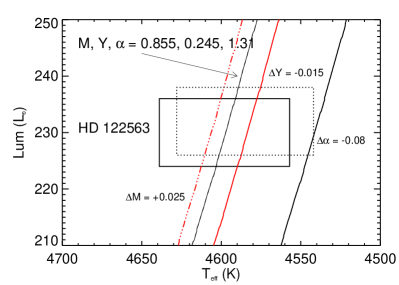
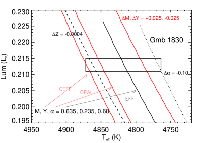
Figure 4: HR diagram showing the observational error boxes for HD 122563 (left) and Gmb 1830 (right). Both figures show stellar models that pass through the error boxes which allow us to determine the stellar model properties and their uncertainties. Each panel shows the adopted central models (with arrows) obtained by considering the HR and metallicity constraints. Other models are also indicated to highlight the parameter uncertainties and correlations. Refer to Sects. 4.3.1 and 4.3.2 for details.

Table 8: Stellar properties and 1$\sigma$ uncertainties derived from modelling HD 122563 (no atomic diffusion) and Gmb 1830 (with atomic diffusion).

	HD 122563	Gmb 1830
Property	EFF EOS		CEFF EOS	OPAL EOS
$M$ (M⊙)	0.855 $\pm$ 0.025	0.635 $\pm$ 0.025	0.625 $\pm$ 0.015	0.620 $\pm$ 0.020
$Y_{\rm i}$	0.245 $\pm$ 0.015	0.235 $\pm$ 0.025	0.230 $\pm$ 0.020	0.235 $\pm$ 0.025
$Z_{\rm i}$/Xi	0.00010 $\pm$ 0.00002	0.0016 $\pm$ 0.0004	0.0016 $\pm$ 0.0004	0.0016 $\pm$ 0.0004
$\alpha$	1.31 $\pm$ 0.08	0.68 $\pm$ 0.10	0.63 $\pm$ 0.08	0.65 $\pm$ 0.10
Age (Gyr)	12.6 $\pm$ 0.1${}^{+1.0}_{-1.5}$	12.1 $\pm$ 0.2${}^{+1.8}_{-2.2}$	12.7 $\pm$ 0.3${}^{+1.3}_{-2.1}$	12.3 $\pm$ 0.3${}^{+1.3}_{-2.3}$
$R$ (R⊙)	24.1 $\pm$ 1.1	0.665 $\pm$ 0.014	0.665 $\pm$ 0.015	0.665 $\pm$ 0.015
$L$ (L⊙)	230 $\pm$ 7	0.213 $\pm$ 0.002	0.213 $\pm$ 0.002	0.213 $\pm$ 0.002
$T_{\rm eff}$ (K)	4598 $\pm$ 42	4815 $\pm$ 52	4814 $\pm$ 53	4815 $\pm$ 50
$\log g$ (dex)	1.60 $\pm$ 0.04	4.60 $\pm$ 0.02	4.59 $\pm$ 0.02	4.58 $\pm$ 0.02
$[$Z/X$]_{s}$	-2.38 $\pm$ 0.10	-1.32 $\pm$ 0.11	-1.32 $\pm$ 0.11	-1.33 $\pm$ 0.11
$\langle\Delta\nu\rangle$${}_{\rm pred}^{a}$ ($\mu$Hz)	1.06 $\pm$ 0.06	198 $\pm$ 6	197 $\pm$ 7	196 $\pm$ 6
$\nu_{\rm max}$${}_{\rm pred}^{a}$ ($\mu$Hz)	5.16 $\pm$ 0.38	4886 $\pm$ 190	4809 $\pm$ 199	4768 $\pm$ 188

Notes: The first five values are the input parameters of the model and the other values are properties of these models. The uncertainties are derived by perturbing each of the model parameters individually until the edge of the error box is reached.
^a$\langle\Delta\nu\rangle$ and $\nu_{\rm max}$ are the predicted seismic quantities according to the scaling relations from Brown & Gilliland (1994); Kjeldsen & Bedding (1995), and the range of values listed consider all the uncertainties in the five model parameters.

4.4 Asteroseismic Constraints

In Table 8 we predict two global asteroseismic quantities $\langle\Delta\nu\rangle$ and $\nu_{\rm max}$ based on scaling relations (Brown & Gilliland 1994; Kjeldsen & Bedding 1995) corresponding to the reference models. Both quantities are proportional to the mass and radius of the star, with the latter also having a small $T_{\rm eff}$-dependence;

$$\hskip 14.22636pt\frac{\langle\Delta\nu\rangle}{\langle\Delta\nu\rangle_{\odot}}\approx M^{0.5}R^{-1.5},\hskip 22.76228pt\frac{\nu_{\rm max}}{\nu_{\rm max,\odot}}\approx\frac{M}{R^{2}\sqrt{T_{\rm eff}/5777{\rm K}}}$$ (1)

where $\langle\Delta\nu\rangle_{\odot}=134.9$ $\mu$Hz and $\nu_{\rm max,\odot}=3,050$ $\mu$Hz (Kjeldsen & Bedding 1995), and $R$ and $M$ are in solar units. Although the relations are approximate, they have been found to work quite well, e.g. Bedding & Kjeldsen (2003); Stello et al. (2008). $\langle\Delta\nu\rangle$ is the characteristic spacing between consecutive radial overtones of the same mode degree seen in the power (frequency) spectrum of a star with sun-like oscillations (e.g. see Fig. 6 from Butler et al. 2004), and it is proportional to the square root of the mean density of the star. Because it is a repetitive pattern (similar to a periodicity), it is relatively easy to determine from even low signal/noise data (see e.g. Huber et al. 2009; Mosser & Appourchaux 2009; Roxburgh 2009; Mathur et al. 2010; Verner et al. 2011 who discuss different methods to determine this value). The value of $\nu_{\rm max}$ is the frequency corresponding to the maximum amplitude of the bell-shaped amplitude/power spectrum, and it is also a quantity that can be more easily observed than, for example, individual oscillation modes.

Because the radii and effective temperatures of these stars are well determined, the predicted seismic quantities depend only on the mass of the star. If we substitute directly the derived mass ranges into the equations then we can predict the range of possible values for these quantities corresponding to the central model, i.e. not taking into account the changes in $\alpha$, $Y_{\rm i}$ or $Z_{\rm i}/X_{\rm i}$. For Gmb 1830  we find that for masses = [0.62, 0.64, 0.66] M_⊙ we calculate $\nu_{\rm max}$ = [4773, 4927, 5081] $\mu$Hz and $\langle\Delta\nu\rangle$ = [196, 199, 203] $\mu$Hz, which correspond to typical periods of approximately 4 minutes. If we can detect these values, even with poor precision we will still be able to select the optimal mass range and discard certain solutions. We note that both $M$ and $Y_{\rm i}$ are very highly correlated, and so fixing $M$ will present interesting constraints on $Y_{\rm i}$. Performing such observations from ground-based instrumentation should yield successful results (e.g. a 2+ meter telescope equipped with a highly efficient and stable spectrograph). For HD 122563 we find for $M$ = [0.84, 0.86, 0.88] M_⊙, $\nu_{\rm max}$ = [5.03, 5.15, 5.26] $\mu$Hz and $\langle\Delta\nu\rangle$ = [1.05, 1.06, 1.07] $\mu$Hz. The dominant periods are approximately 2.5 days, and observations from ground-based instrumentation would be difficult. In order to use asteroseismic data to help constrain the models for HD 122563, we would require seismic data from space-borne instruments, such as with the CoRoT or Kepler missions, to provide the necessary precision and determine the individual oscillation modes.

5 Conclusions

We have determined the $T_{\rm eff}$, $L$, and $R$ of HD 122563 and Gmb 1830 by using $K$ band interferometric measurements (Table 7) and 3D/1D limb-darkening for the giant/dwarf. We find angular diameters of $\theta_{\rm 3D}=0.940\pm 0.011$ mas and $\theta_{\rm 1D}=0.679\pm 0.015$ mas for HD 122563 and Gmb 1830, respectively, and these convert into $T_{\rm eff}$ = 4598 $\pm$ 41 K for HD 122563 and $T_{\rm eff}$ = 4818 $\pm$ 54 K for Gmb 1830. These new precision temperatures increase the well-known difficulty of fitting the error boxes of these two metal-poor stars with evolutionary tracks. Using the CESAM2k stellar structure and evolution code we found that we could match models to the data by using values of the mixing length (the parameter $\alpha$) very different from that of the Sun. We found values of $\alpha$ = 0.68 and 1.31 for the 0.63 M_⊙ dwarf star and the 0.86 M_⊙ giant, respectively. The order of these values seems consistent with recent model analyses (Yıldız et al. 2006; Kervella et al. 2008). We found that different equations of state lead to qualitatively but not quantitively different model parameters for the dwarf star but not for the giant. The initial helium content comes out similar to the big-bang value, the deduced masses are low and their ages are high, consistent with expected values for metal-poor halo stars (see Table 8). The masses are determined with a few percent precision and coupling these with the radii yields well-constrained values of $\log g$. For the giant star we found $\log g$ = $1.60\pm 0.04$ somewhat higher than the typical values (1.1 - 1.5) adopted by spectroscopic analyses according to the PASTEL catalogue (Soubiran et al. 2010) and for the dwarf star we obtain $\log g$ = 4.59 $\pm$ 0.02 dex. Barbuy et al. (2003) determined the O abundance of HD 122563 assuming two different (both justified) values of $\log g$, and they concluded that their resulting [O/Fe] = +0.7 abundance seemed most consistent when they adopt the Hipparcos $\log g$ = 1.5 and not the value determined from ionization equilibrium of Fe, $\log g$ = 1.1, a result due possibly to NLTE effects. This work supports their O determination. With both $\log g$ and $T_{\rm eff}$ now very precisely known, these provide very important inputs for any spectroscopic analyses, especially for the determination of neutron-capture element abundances which can constrain models of nucleosynthesis.

Finally, we have also predicted the asteroseismic signatures $\langle\Delta\nu\rangle$ and $\nu_{\rm max}$ for the two stars and we showed that determinations of these quantities for the dwarf star are possible using ground-based observations. For the giant, however, we would require very long time series in order to resolve the frequency content of the oscillations, and this would only be possible with space-borne instruments. The asteroseismic data would provide very important constraints because it would allow us to determine the mass with better precision (using the radius from this work), and thus the initial helium abundance.