Temporal Evolution of Velocity and Magnetic Field in and around Umbral Dots

Abstract

We study the temporal evolution of umbral dots (UDs) using measurements from the CRISP imaging spectropolarimeter at the Swedish 1-m Solar Telescope. Scans of the magnetically sensitive 630 nm iron lines were performed under stable atmospheric conditions for 71 min with a cadence of 63 s. These observations allow us to investigate the magnetic field and velocity in and around UDs at a resolution approaching 0$\farcs$13. From the analysis of 339 UDs, we draw the following conclusions: (1) UDs show clear hints of upflows, as predicted by magnetohydrodynamic (MHD) simulations. By contrast, we could not find systematic downflow signals. Only in very deep layers we detect localized downflows around UDs, but they do not persist in time. (2) We confirm that UDs exhibit weaker and more inclined fields than their surroundings, as reported previously. However, UDs that have strong fields above 2000 G or are in the decay phase show enhanced and more vertical fields. (3) There are enhanced fields at the migration front of UDs detached from penumbral grains, as if their motion were impeded by the ambient field. (4) Long-lived UDs travel longer distances with slower proper motions. Our results appear to confirm some aspects of recent numerical simulations of magnetoconvection in the umbra (e.g., the existence of upflows in UDs), but not others (e.g., the systematic weakening of the magnetic field at the position of UDs.)

1. Introduction

Umbral dots (UDs) are transient brightenings observed in sunspot umbrae and pores, with typical sizes of 300 km and lifetimes of 10 min (e.g., Sobotka et al., 1997a, b). They cover only 3–10% of the umbral area, but contribute 10–20% of its brightness. For this reason, UDs are believed to play a vital role in the energy balance of sunspots (Deinzer, 1965; Sobotka et al., 1993; Moradi et al., 2010).

UDs exhibit systematic proper motions in mature sunspots: those appearing in the central umbral region are static, while UDs in peripheral regions move inward with an average velocity of 1.0  km s^-1 (Kitai et al., 2007; Riethmüller et al., 2008b). Some peripheral UDs are the continuation of penumbral grains—bright elongated structures at the head of penumbral filaments that move toward the center of the sunspot with speeds of about 0.4  km s^-1 (Sobotka et al., 1999a; Rimmele & Marino, 2006). When the migration front detaches into a circular bright point, the tip of the penumbral grain becomes an UD.

It is believed that the mechanism behind UDs is convection interacting with the strong vertical field of the umbra, and many observational results support this idea (Riethmüller et al., 2008a; Bharti et al., 2010; Watanabe et al., 2010). In the formation phase of sunspots, UDs are akin to granules but their apparent motion is more stochastic because of the surrounding magnetic field (Sobotka et al., 1999b). In developed sunspots, UDs are small and quiescent due to the stronger suppression of convection.

UD research is entering a new phase in which computer simulations guide observational efforts. The innovative simulations by Schüssler & Vögler (2006) predicted UDs with central dark lanes and small localized downflow patches at their ends. A clear detection of those features would immediately validate the numerical models, so they have been the target of recent observations. The dark lanes are the result of enhanced density in the upper central part of UDs, caused by the piling up of hot gas that rises from deeper down. Once the gas reaches the surface, it cools by radiative losses and descends in narrow downflow channels at the end of the dark lanes. Bharti et al. (2007b) observed a dark lane in a big UD. However, the very large size of this UD ($>$1000 km) suggests that it could actually have been a cluster of several UDs. The first detection of downflows surrounding an UD was presented by Bharti et al. (2007a). Subsequently, Ortiz et al. (2010) reported solid evidence of dark lanes and localized downflows based on spectropolarimetric observations taken at the Swedish 1-m Solar Telescope. The sizes of the dark lanes and downflowing patches found by Ortiz et al. (2010) are near the diffraction limit of the telescope, with the substructures keeping their identity for periods of only a few minutes. These authors also reported enhanced net circular polarization at the site of the downflows.

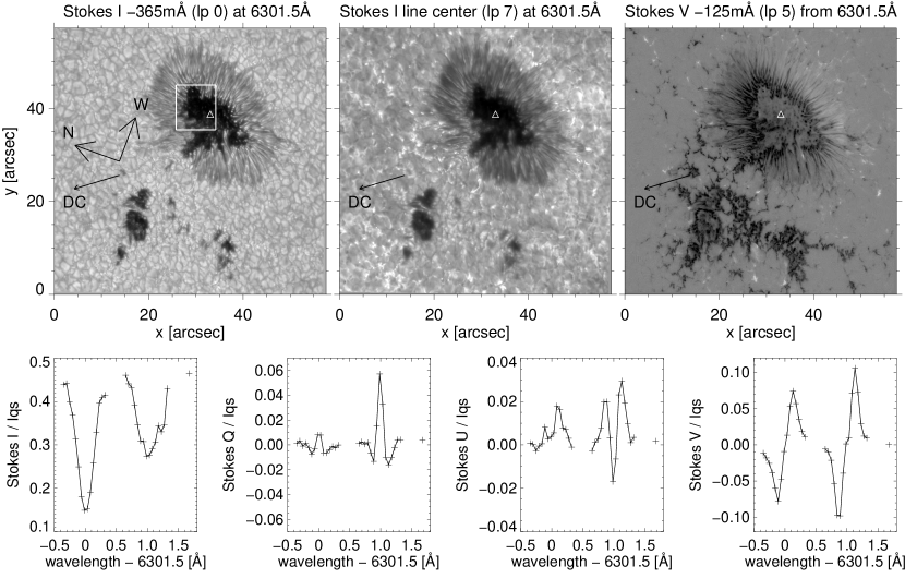
Figure 1.— Filtergrams from the best scan of the data set, taken at 08:30 UT. The full FOV is shown. From left to right: Stokes $I$ in the blue wing of 6301.5 Å (line position 0), Stokes $I$ at line center (line position 7), and Stokes $V$ in the blue wing (line position 5). The direction to disk center (DC) is displayed with an arrow. The white rectangle indicates the FOV of Figure 2. The bottom row shows the Stokes profiles emerging from the UD marked with triangles in the upper panels. The $+$-symbols indicate the measured signals.

The evolution of UDs and their magnetic fields is difficult to study—and hence poorly known—because one needs full vector spectropolarimetric measurements at very high temporal and spatial resolution. To the best of our knowledge, the magnetic properties of UDs have never been investigated at the required cadence and spatial resolution (but see Sobotka & Jurčák, 2009). Ortiz et al. (2010) performed a preliminary analysis of the temporal evolution of six UDs, and this work should be considered a substantial extension of their study. Both the cadence and the polarimetric sensitivity of our measurements are improved with respect to those of Ortiz et al. (2010), as is the total duration of the observations, 71 minutes, during which the seeing conditions were excellent and stable. We use this unique data set to investigate the evolution of the magnetic and velocity fields in and around UDs.

The paper is organized as follows. The observations are described in Section 2, followed by an account of the methods used for the detection of UDs and derivation of the velocity and magnetic information (Section 3). In Section 4 we quantify how convection is modified in the umbra. In Section 5 we describe the evolution of some typical UDs, and present the results of our statistical analysis. Finally, based on these results, we discuss the physical properties of UDs in Section 6.

2. Observations and Data Reduction

The observations were obtained with the CRisp Imaging Spectro-Polarimeter (CRISP) at the Swedish 1-m Solar Telescope (SST; Scharmer et al., 2003) on La Palma, Spain. CRISP is based on a dual Fabry-Pérot interferometer similar to that described by Scharmer (2006). The incoming light is modulated by two liquid crystal variable retarders cycling through four states and then analyzed by a polarizing beam splitter in front of two narrow-band cameras. The narrow-band cameras record orthogonal polarization states to minimize seeing-induced crosstalk. CRISP has a third camera for wide band imaging. All the cameras operate at 35 frames per second and take exposures of 17.6 ms. The synchronism between them is ensured by an external optical chopper.

CRISP was used to measure the four Stokes profiles of the magnetically sensitive Fe I 6301.5 and 6302.5 Å lines, each sampled at 15 wavelength positions in steps of 48 mÅ, from $-$350 to $+$322 mÅ. Line positions 0–14 sample the 6301.5 Å line, while positions 15–29 correspond to the 6302.5 Å line. In addition, a continuum wavelength point (6303.2 Å, line position 30) was measured. We recorded 9 frames per modulation state, resulting in 36 exposures per wavelength position. The total time for a complete wavelength scan of the two Fe I lines plus the continuum point was 32 s. Another 30 s were needed to scan the Ca II line at 8542 Å (not used in this paper). Thus, the temporal cadence of the Fe I scans is 63 s. The average CRISP transmission profile has a Gaussian core (FWHM of 64 mÅ at 6300Å) and wide Lorentzian wings. This transmission profile reduces the line core depth of the Fe I lines by about 20%.

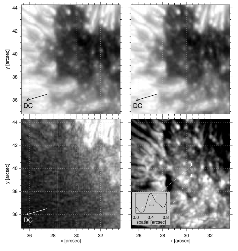
Figure 2.— Close-up of the region indicated with a white box in Figure 1. Clockwise, starting from upper left: intensity in the blue wing of Fe I 6301.5 Å (line position 0), continuum intensity at 6303.2 Å (line position 30), CP map, and LP map. The direction to disk center (DC) is displayed with an arrow. A cut of a point-like feature (corresponding to an UD) is shown in the CP map. The length of the arrow in the plot is 0$\farcs$13 (equal to the diffraction limit).

The CRISP etalons are mounted in tandem on a telecentric beam. The separation of the cavities of the high resolution etalon sets the wavelength of the transmission profile. This is not strictly the same over the whole field of view (FOV) because the surface cannot be infinitely flat, producing random wavelength shifts (cavity errors) across the FOV. Intensity fluctuations, introduced by cavity errors in the presence of a spectral line, were removed from the flat-field images in a similar way as described by Schnerr et al. (2011). Their flat-fielding scheme computes a cavity-error-free averaged quiet-sun profile, which is removed from the flats on a pixel-by-pixel basis. This average is obtained by summing many hundreds of exposures acquired by moving the telescope in circles around the disk center. The difference between the Schnerr et al. (2011) scheme and ours is that we applied a polarization-free flat for all the four Stokes states taken at one wavelength position.

We also corrected the data for spectral intensity gradients introduced by the CRISP prefilter. The prefilter correction can be decomposed in two contributions, an average prefilter shape and a term that accounts for pixel-to-pixel deviations:

$$P(\lambda,x,y)=P_{\rm g}(\lambda)+{\rm d}P(x,y).$$ (1)

The second term of the equation is included in the flat-field correction. To obtain the global prefilter shape ($P_{\rm g}$), our estimate of the averaged quiet-sun profile is compared to the FTS atlas convolved with the CRISP transmission profile. The prefilter is assumed to have a Lorentzian shape which is multiplied with a polynomial term to account for asymmetries:

$$P_{\rm g}(\lambda)=\frac{1}{1+[2(\lambda-\lambda_{0})/w]^{2N_{\rm cav}}}\,(1+p_{0}\lambda+p_{1}\lambda^{3}).$$ (2)

Here, $\lambda_{0}$ and $w$ are the central wavelength and FWHM of the prefilter, respectively, $N_{\rm cav}$ is the number of cavities of the filter ($N_{\rm cav}=2$ in this case), and $p_{0}$ and $p_{1}$ are the coefficients of the polynomial. A least-squares-fitting scheme (Markwardt, 2009) was used to compute the prefilter parameters, minimizing the differences between the observed and modeled curves. All Stokes parameters were then corrected by dividing each spectrum with the fitted prefilter curve.

The theoretical diffraction limit of the telescope around 6300 Å is 0$\farcs$13, and the image pixel size is 0$\farcs$059. To ensure very high spatial resolution, we used the adaptive optics system of the SST and the Multi-Object Multi-Frame Blind Deconvolution technique (MOMFBD; van Noort et al., 2005). The MOMFBD algorithm considers all frames taken in one scan (31 wavelength points $\times$ 4 modulation states $\times$ 9 repetitions $\times$ 3 cameras) to remove image distortions from the individual filtergrams.

Under enhanced differential-seeing conditions, residual rubber sheet distortions are present between the narrow-band images of the same scan even after MOMFBD restoration. This effect appears when the size of the patches used to divide the images for the MOMFBD processing (here $128\times 128$ pixels) is larger than the spatial scale of the atmospheric distortion (or iso-planatic patch). To attenuate their influence in our measurements, we employed an extra step in the processing following an idea from V. Henriques (private communication). The wide-band images were used twice in a MOMFBD restoration in the following manner:

1. All the frames were combined to produce the reference anchor image.

2. The frames were separated in sets associated with each wavelength position and modulation state, resulting in one restored wide-band image per wavelength and modulation state.

The second set of wide-band images was not used for wavefront sensing, i.e., they did not contribute to the determination of the Point Spread Function in the MOMFBD calculations. The state-dependent restored wide-band images were compared with the anchor wide-band image to remove the residual rubber sheet deformations in the individual filtergrams. This correction was applied prior to the demodulation of the data to achieve almost perfect co-alignment between the 4 modulation states from which the Stokes parameters are derived at any wavelength position. The method also achieves almost perfect co-alignment between the different wavelength positions to ensure the integrity of the Stokes profiles over the FOV.

After restoration, the images were demodulated and corrected for instrumental polarization using the telescope model developed by Selbing (2010). For details, see van Noort & Rouppe van der Voort (2008). In addition, we corrected small residual crosstalks from Stokes $I$ to $Q$, $U$, and $V$ by forcing the polarization to be zero in the far line wings. All the Stokes profiles were normalized to the average quiet-sun continuum intensity ($I_{\rm qs}$) computed for each time step. The typical noise levels in Stokes $Q$, $U$, and $V$ are $1.9\times 10^{-3}$, $2.8\times 10^{-3}$, and $1.9\times 10^{-3}$ of the continuum intensity, respectively.

We followed the main sunspot of NOAA active region 11024 from 08:05 to 09:16 UT on 6 July 2009. The spot was located at 25^∘S and 23^∘W (heliocentric angle of 36^∘, $\mu$=0.81). During the observations the atmospheric conditions were excellent and stable. Figure 1 shows selected filtergrams from one of the best scans (08:30 UT) and the four Stokes profiles measured at the position of an UD. The size of the full FOV is $58\arcsec\times 57\arcsec$.

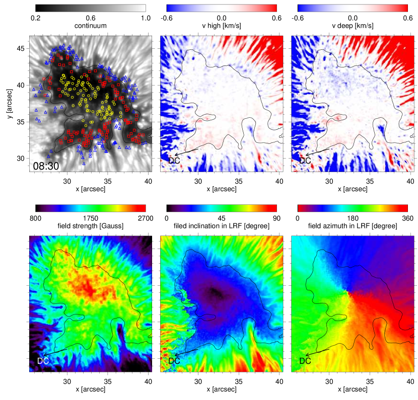
Figure 3.— Physical parameters derived from the observed Stokes profiles. Shown in the figure is the scan with best seeing conditions, taken at 08:30 UT. The top panels, from left to right, display the continuum intensity map with the position of appearance of all the detected UDs (yellow circles are central UDs, red squares are peripheral UDs, blue triangles are grain-origin UDs), and two bisector maps sampling high ($v_{\rm high}$) and deep ($v_{\rm deep}$) photospheric layers. Negative velocities (blue) represent upflows along the line of sight, while positive velocities (red) mean downflows. The bottom panels, from left to right, show the field strength, the field inclination, and the field azimuth in the local reference frame (LRF). The black contours indicate the approximate umbral boundary defined by the spatially-smoothed continuum intensity. The arrows mark the direction to disk center (DC). An mpeg version of this figure is available in the on-line journal.

Figure 2 displays a close-up of the umbra and the inner penumbra on the disk-center side of the spot. The maps of mean linear polarization (LP) and circular polarization (CP) degree were calculated as

$${\rm LP}=\frac{\int{[Q^{2}(\lambda)+U^{2}(\lambda)]^{1/2}\,/\,I(\lambda)}\,{\rm d}\lambda}{\int{{\rm d}\lambda}},$$ (3)

$${\rm CP}=\frac{\int{|V(\lambda)|\,/\,I(\lambda)}\,{\rm d}\lambda}{\int{d\lambda}},$$ (4)

with the integration extending over the Fe I 6301.5 Å line. The LP signals are stronger toward the limb due to projection effects. Most of the fine-scale structures seen in the LP and CP maps coincide with UDs. Figure 2 clearly demonstrates that

1. The first and last intensity images of the scan are perfectly aligned and do not show distortions in spite of the fact that they were taken about 30 s apart (top row). This confirms the good performance of the MOMFBD processing.

2. Almost all UDs in the umbra keep their brightness, size, and position during the line scan (top row), that is, the scan time is shorter than the dynamic timescale of UDs.

3. The smallest features visible in the maps (UDs and dark cores of penumbral filaments) are only slightly larger than the diffraction limit of the SST. They show higher contrasts in circular polarization.

We believe this is one of the best UD data sets ever obtained, because of its superb spatial resolution (0$\farcs$13), the stable seeing conditions, and the availability of two-dimensional spectropolarimetric measurements for more than 70 minutes with good temporal cadence (63 s). The non-simultaneous acquisition of spectral information—the main disadvantage of Fabry-Pérot systems—can be well neglected because UDs evolve on time scales longer than the scan time.

3. Data analysis

In this section we describe the methods we have used to detect and track UDs, as well as the line bisector calculations and Stokes inversions performed to derive their velocities and magnetic fields.

3.1. Detection and Categorization

For the statistical study of UDs it is convenient to use automatic detection algorithms (Sobotka et al., 1997a; Bharti et al., 2010). However, we have implemented a manual procedure here because, even under the very stable seeing conditions of our observations, the image quality still shows an unavoidable amount of residual fluctuation which might compromise the performance of automatic methods.

The procedure works as follows. First we inspect the continuum movie to identify the frame of appearance of each UD. The position of the UD is then tracked by clicking on the screen until it disappears. After going through the temporal sequence, we run the movie backward in time to check the consistency. When an UD splits in two fragments, the bigger component is the one that continues to be tracked and the smaller component is selected separately as a new entity. When two UDs merge, the smaller is assumed to die. In some cases, UDs show recurrence at the same position. If the recurrent UDs appear within an interval of 3 frames ($\sim$3 min), we consider them a single entity.

UDs evolving from penumbral grains are also studied. In this case, the detection starts from the frame in which the tip of the penumbral grain detaches from the filamentary structure. Sometimes these UDs are connected to the penumbral grains through a faint tail, but they become more isolated and roundish as they move toward the umbra.

This method has allowed us to obtain the trajectories of 339 UDs. According to their place of birth, we categorize them into three groups. UDs located in the central part of the umbra are called “central UDs” (98 samples out of 339 UDs), UDs located in the peripheral area are called “peripheral UDs” (112 samples), and UDs detached from penumbral grains are called “grain-origin UDs” (129 samples). The peripheral area is an $\sim$1–2 ″ annular region adjacent to the umbra-penumbra boundary. It is known that central UDs are static while peripheral and grain-origin UDs show a systematic motion toward the center of the umbra (Ewell, 1992; Sobotka et al., 1997b). About 40% of the 339 UDs we have detected did not appear or disappear within the interval covered by the observations. Therefore, their lifetimes could not be computed.

Table 1 Average properties of UDs

Parameter	Central	Peripheral	Grain-origin
Number	98	112	129
Lifetime [min]	19	18	17
Proper motion [ km s-1]	0.19	0.31	0.49
Brightness ratio	1.46	1.50	1.89
Diameter [km]	401	391	482

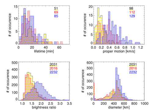
Figure 4.— Histograms of UD lifetime (upper left), average proper motion speed (upper right), brightness ratio (lower left), and diameter (lower right). Central UDs are displayed with black bars filled with yellow color, peripheral UDs with red color, and grain-origin UDs with blue color. The number of measurements in each category is shown in the upper-right corner of the histograms.

In the upper left panel of Figure 3 we show the position of appearance of all 339 UDs. The yellow circles indicate central UDs, the red squares peripheral UDs, and the blue triangles grain-origin UDs. Table 1 lists their mean properties. The average lifetime is about 18 min. This is relatively long compared with the values reported in previous works (e.g., Riethmüller et al., 2008b), probably because our manual procedure is capable of detecting fainter UDs. UDs move with an average speed of 0.2-0.5  km s^-1. The proper motion speed is defined as the distance between the points of appearance and disappearance divided by the time interval. Distances are not corrected for projection effects. The brightness ratio is the UD intensity (the maximum intensity within a $\pm$2 pixel area) relative to the intensity of the dark background ($I_{\rm db}$). We use the “dark background”—the region surrounding the UD but excluding the UD itself—as a local reference. $I_{\rm db}$ is the mean intensity of pixels over a $2\arcsec\times 2\arcsec$ area centered in the UD whose intensity is darker than the average minus 0.5$\sigma$. Here, $\sigma$ represents the standard deviation of the intensity within the $2\arcsec\times 2\arcsec$ area. We find average brightness ratios from 1.5 (central UDs) to nearly 1.9 (grain-origin UDs). The mean UD diameter is 400–500 km. For each UD, the diameter is calculated as the average distance in eight radial directions along which the intensity is brighter than $1.2\,I_{\rm db}$, or as the distance to the closest inflection point. A similar method was adopted in Watanabe et al. (2009a). There are some instances of zero diameter, which means that the UD intensity was darker than $1.2\,I_{\rm db}$. Brightness ratios and diameters are calculated for every time step within the UD lifetime, so in total we get 6279 individual values.

Figure 5.— Intensity profiles emerging from the tip of a penumbral grain (pluses) and from an UD (asterisks). The diamonds indicate the bisector positions at intensity levels of 10% and 23% (constituting $v_{\rm high}$), and 49% and 62% (constituting $v_{\rm deep}$).

Figure 4 shows histograms of these parameters for all the UDs detected in the observations. Central and peripheral UDs are very similar except that the latter move faster. Grain-origin UDs, however, are clearly different: they have the fastest speeds, the highest intensity contrasts, and the largest diameters.

3.2. Derivation of Velocities: Line Bisectors

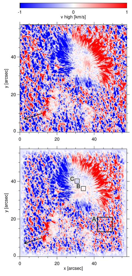
Figure 6.— Original $v_{\rm high}$ map observed at 08:31 UT (top) and subsonic filtered map (bottom). Negative velocities (blue) mean upflows along the line of sight, and positive velocities (red) mean downflows. The arrows mark the direction to disk center. The regions labeled A–C will be studied in Section 4.2.

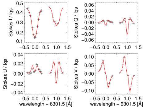
Figure 7.— Stokes profiles observed at the position of an UD (marked with a triangle in Figure 1) and best-fit profiles returned by SIR (symbols and red solid lines, respectively).

The mean wavelength position of the two line wings at a given intensity level is called the line bisector (Figure 5). Since different intensity levels sample different atmospheric layers, bisectors are often used to estimate the height variation of the line-of-sight velocity (e.g., Tritschler et al., 2004; Ortiz et al., 2010). The 0% intensity level represents the line core, while 100% means the local continuum.

We calculate bisectors only for Fe I 6301.5 Å because the red wing of Fe I 6302.5 Å is strongly blended with the telluric O₂ 6302.8 Å line (see the Stokes $I$ profile in Figure 1). The Fe I 6301.5 Å line is less affected by blending, although its far blue wing (intensity levels $>70\%$) sometimes show influence of molecular lines in the darkest umbral areas (Martínez Pillet & Vázquez, 1993), which may result in a systematic blueshift. For this reason we calculated four bisector positions at intensity levels of 10%, 23%, 49%, and 62%, avoiding bisectors close to the continuum. Each bisector position is obtained from a linear interpolation of the relevant intensities in the observed line profile. To reduce the noise, two bisector levels are averaged. As can be seen in Figure 5, this results in two bisector velocities which will be called $v_{\rm high}$ (10% and 23%) and $v_{\rm deep}$ (49% and 62%). The $v_{\rm high}$ and $v_{\rm deep}$ maps are not corrected for projection effects, but they mostly represent vertical flows because horizontal flows are usually weak in the solar photosphere. Negative values of $v_{\rm high}$ and $v_{\rm deep}$ correspond to blueshifts (or upflows along the line of sight), and positive values to redshifts (or downflows).

Following Title et al. (1989), we apply a subsonic Fourier filter to the temporal sequence of $v_{\rm high}$ and $v_{\rm deep}$ to suppress disturbances with horizontal speeds larger than 4  km s^-1, which are mostly due to $p$-modes and the residual temporal noise. In the umbra, a large scale ($\sim$5000 km) velocity pattern corresponding to the $p$-mode oscillations is observed. This pattern is removed by the filter. We use an edge apodization of 10% in space and time to avoid the propagation of boundary errors. The effect of the subsonic filtering is demonstrated in Figure 6. The dominant redshift signal on the right side of the umbra at $(x,y)\sim(37\arcsec,37\arcsec)$ in the original image (upper panel) is absent in the filtered image (lower panel). However small local variations, which coincide with the UD’s positions, keep their identity even after the subsonic filtering.

For both $v_{\rm deep}$ and $v_{\rm high}$, the zero velocity is determined by averaging the filtered $v_{\rm high}$ map over umbral pixels with intensities below $0.4\,I_{\rm qs}$. This is done for each of the 68 frames of the sequence. The $v_{\rm high}$ and $v_{\rm deep}$ maps look similar, but the latter shows larger root-mean-square (rms) fluctuations. The typical rms velocities in the umbra are 0.11  km s^-1 for $v_{\rm high}$ and 0.13  km s^-1 for $v_{\rm deep}$. The rms variations increase significantly when the maps are not filtered. Thus, the filtering is essential to provide a good velocity reference, and also to remove the large velocity offsets induced by the $p$-mode oscillations. This is particularly important when dealing with small velocities such as those observed in UDs.

3.3. Derivation of Magnetic Properties: Stokes Inversion

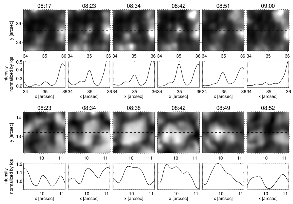
Figure 8.— Temporal evolution of a central UD (top) and a quiet Sun granule (bottom). Displayed are continuum intensity maps for an area of $2\farcs 2\times 2\farcs 2$. The coordinate system coincides with that of Figure 1. An intensity cut along the dashed line plotted at the center of the FOV is shown below each image. Times are given in UT in the intensity panels.

We determine the magnetic properties of the umbra by inverting the observed Stokes profiles with the SIR code (Stokes Inversion based on Response functions; Ruiz Cobo & del Toro Iniesta, 1992). The two lines are fitted simultaneously, excluding the telluric O₂ blend in the red wing of the Fe I 6302.5 Stokes $I$ profile.

The inversion is carried out in terms of a one-component model atmosphere with constant (i.e., height-independent) magnetic fields and velocities, which is sufficient to explain the relatively symmetric Stokes profiles observed in the sunspot umbra (see Figure 7). Zero stray-light contamination and unity magnetic filling factors are assumed. The inversion returns 9 free parameters: the three components of the vector magnetic field (strength, inclination, and azimuth), the line-of-sight velocity, the microturbulent velocity, and the temperature at 4 nodes. The initial guess model used to start the inversion is the hot umbral model of Collados et al. (1994).

Sample maps of the retrieved magnetic parameters are displayed in Figure 3. The inclination and azimuth angles are expressed in the local reference frame to avoid projection effects. The inclination varies from $0^{\circ}$ to $180^{\circ}$ for vertical fields pointing away from and to the solar surface, respectively. The azimuth is measured counterclockwise from the positive $x$-axis of the figure. As expected, the sunspot shows an outward-directed radial magnetic field. We also note that the line-of-sight velocities returned by the inversion agree well with the bisector velocities obtained from the 6301.5 Å line. An animated version of Figure 3 is available in the on-line journal.

4. Convection in the Umbra

In the solar photosphere, the presence of strong magnetic fields inhibits convective energy transport. This is why sunspots are dark and cool compared to the quiet Sun, which is covered by convective cells called granules. However, convection is not entirely suppressed even in the umbra: as a matter of fact, UDs are the manifestation of a modified convective pattern. The properties of this pattern still need to be determined. Here we study how the characteristics of convection differ between the quiet Sun and the umbra, paying special attention to the morphology of the convective cells and the correlation between brightness and velocity.

4.1. Morphology

Figure 8 illustrates the morphological evolution of a central UD and a quiet-Sun granule. The images cover an area of $2\farcs 2\times 2\farcs 2$. First we notice that the UD is much smaller than the granule ($\sim$0$\farcs$3 vs 1$\farcs$0; cf., Roudier & Muller, 1987). Second, UDs are relatively isolated whereas granules are closely packed between narrow ($\sim$0$\farcs$3) intergranular lanes. Third, the intensity profile of granules is flat-top, sometimes with intensity depressions in the middle. A granule loses its identity (or disappears) by fragmentation or by merging with neighboring granules. On the other hand, the intensity profile of UDs has a Gaussian shape, and they disappear mostly by fading out.

Both granules and UDs exhibit a turbulent character: the structures displayed in Figure 8 change their brightness, barycenter, and shapes on timescales of only a few minutes. The variations are more pronounced in the case of granules. The average lifetime of UDs, 18 minutes, is slightly longer than the 5–15 minute duration of granules (e.g., Bahng & Schwarzschild, 1961; Alissandrakis et al., 1987; Title et al., 1989; Hirzberger et al., 1999).

Figure 9.— Bisector velocity $v_{\rm high}$ vs continuum intensity for selected umbral and quiet Sun areas using the line scans taken at 08:28 UT (left column) and 08:33 UT (right column). Negative velocities represent upflows along the line of sight. The positions of areas A–C are indicated in Figure 6. $k$ is the slope of the best linear fit and $r$ the Pearson correlation coefficient.

4.2. Brightness vs Velocity

The strong correlation between brightness and line-of-sight velocity in granular convection is well known. Bright areas (i.e., granules) show upflows, while dark areas (the intergranular lanes outlining the granules) harbor downflows. This is illustrated in the top panels of Figure 9.

In the umbra, in addition to UDs, there exist diffuse areas with enhanced brightness. These areas may correspond to a convective pattern similar to (but weaker than) that of the quiet Sun, with UDs being another manifestation of the same pattern occurring at positions where convection is more vigorous. To test this possibility, we have examined the correlation between brightness and velocity in the umbra: if bright structures are the result of convection, then they should preferentially be associated with upflows. The middle and bottom panels of Figure 9 show scatter plots for two umbral areas labeled B and C in Figure 6. Area B is close to the light bridge and C represents the central umbra. In both areas, at 08:28 UT (left column) we find a tendency of upflows in bright regions and downflows in dark regions similar to that of the quiet Sun, yet with weaker correlation. For most of the scans with good seeing conditions, the slope $k$ of the best linear fit to the velocity-brightness relation turns out to be negative, with average values of $-0.11\pm 0.02$ in area B and $-0.24\pm 0.04$ in area C. However, the negative correlation does not always persist in time and scans obtained a few minutes apart under good seeing conditions sometimes show opposite behaviors (compare the lower panels of Figure 9). For this reason, the present data do not allow us to unambiguously confirm the existence of a global convective pattern in the umbra. We will see later that the situation is different for UDs.

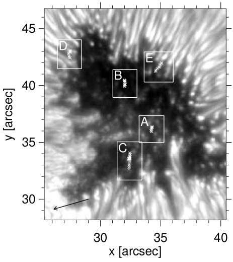
Figure 10.— Position of selected UDs (A-B: central UDs, C: peripheral UD, D-E: grain-origin UDs). The background image shows the continuum intensity at 08:30 UT. The cross symbols indicate the trajectories of the UDs. The arrow marks the direction to disk center.

5. Umbral Dots

In this Section we give a detailed description of the evolution and statistical properties of individual UDs.

5.1. Case Studies

We select five UDs (UD#A–E) whose locations are indicated in Figure 10. All of them were observed from appearance to disappearance. Movies of their temporal evolution can be found in the electronic journal.

In Section 5.1.5, another two UDs from one of the best scans of the sequence will be considered. We use them to demonstrate the existence of localized downflow patches around UDs in deep photospheric layers.

5.1.1 Typical Central UD

According to our visual inspection, more than 70% of the central UDs do not show flow field perturbations, i.e., no upflows or downflows are detected. Similarly, magnetic field perturbations associated with central UDs are usually not visible or very small. 17% of the central UDs split or merge with neighboring UDs.

The temporal evolution of a typical central UD (UD#A) is displayed in Figures 17 and 18. Figure 17 shows maps of physical parameters starting 2 frames before the appearance of the UD (T=0 s) and ending 2 frames after its disappearance. In the left column of Figure 18, curves representing the temporal variation of the parameters at the position of the UD (solid line) and the dark background (dashed line) are given. The curve for the dark background is an average over pixels with intensities lower than the average minus $0.5\sigma$ in the FOV of Figure 17. The right column of Figure 18 shows spatial profiles along the $x$-direction at $y$-positions co-moving with the UD. The Gaussian peak at $x=34\farcs 3$ in the continuum plot corresponds to the UD.

UD#A was born in a diffuse bright region, then increased in brightness (0 s$<$T$<$377 s), and finally merged with a neighboring UD (755 s$<$T$<$1006 s). As can be seen in both maps and plots, it did not show clear upflows or downflows. During most of its lifetime, the UD was located in a patch of enhanced redshifts whose morphology and amplitude do not correlate with the UD evolution. Other UDs in the FOV display localized upflows of up to $v_{\rm deep}$ $=$ 0.3  km s^-1, but they do not persist in time. An example is the structure located next to UD#A at coordinates (34$\farcs$1, 36$\farcs$6), between $T=566$ and 755 s. In Figure 17, a local reduction of the field strength at the position of UD#A can be seen during 0 s$<$T$<$629 s. Then, the UD appears to gradually merge with a pre-existing weak field patch right above it. The amplitude of the magnetic field perturbations is very small, about 50 G. The UD does not leave clear signatures in the inclination maps.

5.1.2 Distinct Central UD

Figures 19 and 20 show the temporal evolution of a distinct central UD (UD#B). This UD differs from the others because of its large brightness and upflow. UD#B was born in a very dark area within the umbra and the continuum intensity became quite high about 9 minutes later (566 s$<$T$<$880 s). A second smaller intensity peak appeared in the interval 1069 s$<$T$<$1321 s. Finally the UD faded in a diffuse bright background with no detectable intensity peak. There was a significant upflow associated with the continuum intensity enhancement. The maximum upflow of $v_{\rm high}$ $\sim 0.3$  km s^-1 occurred at T=755 s. A reduction of the field strength of the order of 50 G co-spatial with the UD can be observed during the first half of its lifetime. After T=755 s, the region of weaker field strengths disappears and the UD collides with a pre-existing strong field region. Sometimes there is a small spatial displacement (up to 0$\farcs$2) between the brightness peak and the patch of reduced field strengths. A very small patch with more inclined fields appeared transiently from $T=566$ to 755 s.

The bright UD located at coordinates $(31\farcs 5,40\arcsec)$ also showed reduced field strengths and strong upflows (particularly in $v_{\rm high}$) for more than 6 minutes, from $T=-125$ to 251 s.

5.1.3 Typical Peripheral UD

Peripheral UDs are born in the peripheral region of the umbra, where the continuum intensity is brighter and the magnetic field more inclined. A significant property of peripheral UDs is their systematic motion toward the center of the umbra (see Table 1). Our visual inspection reveals that 55% of the detected peripheral UDs show upflows, but no systematic magnetic field perturbations. For example, 13% of peripheral UDs present a reduction of field strength, while 16% of them are associated with enhanced fields. Usually, these perturbations do not last more than a few minutes.

Figures 21 and 22 display the evolution of UD#C, a typical peripheral UD. The inward migration of this UD is very clearly seen in the online animation. The migration speed is $\sim$1.1  km s^-1 during 0 s$<$T$<$503 s, and almost zero during 503 s$<$T$<$1635 s. In the final stages of its life (1635 s$<$T$<$2390 s), the UD migrates again with a speed of 0.5  km s^-1. The origin of UD#C is a diffuse bright area within the umbra. It shows three brightness peaks: at $T=377$, 1132, and 1761 s. Only the first is associated with strong upflows ($v_{\rm high}$ $\sim-0.15$  km s^-1 and $v_{\rm deep}$ $\sim-0.35$  km s^-1). The other two peaks show much smaller velocities, but still shifted to the blue compared with the dark background. A hint of redshifts can be seen in $v_{\rm deep}$ from T$=$2202 to 2390 s.

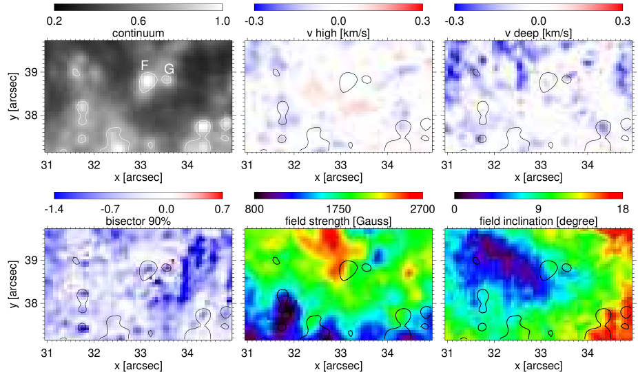
Figure 11.— Close-up images of the central area of the umbra from the line scan taken at 08:30 UT. Clockwise, starting from top left: continuum intensity, $v_{\rm high}$, $v_{\rm deep}$, field inclination, field strength, and bisector velocity at the 90% intensity level. Negative velocities represent upflows along the line of sight. The contours show continuum intensities of $0.4\,I_{\rm qs}$.

The magnetic field shows a complex distribution. A patch of reduced field strength ($\sim-100$ G) develops at the position of the UD and migrates inward to the umbra during 377 s$<$T$<$1069 s. The magnetic field perturbation then disappears. At T$=$1635 s the negative patch can be observed again at the position of the UD. It will survive for most of the remaining UD’s evolution. In addition, another patch of increased field strengths is visible to the left of the UD, at $(x,y)\approx(32\arcsec,33\arcsec)$. This structure already exists from T=$-$125 s (before the appearance of UD#C) and also migrates inward, but with slower speed (0.5  km s^-1 during 0 s$<$T$<$755 s). The patch disappears when the UD’s brightness decreases at around T$=$2202 s. The vector magnetic field of UD#C gets more inclined, especially during the migration.

5.1.4 Typical Grain-Origin UDs

Grain-origin UDs are characterized by inward migration to the umbra center and high intensity contrasts (Table 1). The perturbations associated with these UDs are more clearly visible than those of central and peripheral UDs. Our analysis demonstrates that more than 70% of the grain-origin UDs harbor upflows, while 40–50% show weaker and more inclined fields. The magnetic field perturbations occur preferentially near the penumbra, becoming less prominent as the UD moves into the umbra. Sometimes one observes patches of both reduced and increased field strengths at the position of grain-origin UDs.

In this section we describe the evolution of two typical grain-origin UDs: one from the disk center side of the spot and the other from the limb side.

Figures 23 and 24 show the temporal evolution of the disk-center side UD (UD#D). It evolves from a filamentary structure into a circular shape and follows an unusual trajectory: generally, grain-origin UDs move along the extension line of penumbral grains, but the trajectory of UD#D is almost perpendicular to it. The continuum intensity decreases a bit during 188 s$<$T$<$314 s, and then increases again. Upflows are observed in the first half of the UD evolution, weakening until they almost reach the background level at $T=692$ s. The strongest flow ($v_{\rm deep}$$<-0.6$  km s^-1) occurs at the edge of the penumbral grain early in the UD’s evolution, around $T=62$ s, and appears to be the continuation of the typical upflow of penumbral grains.

UD#D is located at the boundary of weak and strong field regions. When it moves along the $-y$ direction, the boundary also evolves as if the leading edge of the UD was always blocked by strong field walls (0 s$<$T$<$817 s). After that, the UD collides with the strong field region and then disappears together with the strong field walls. We could not detect any systematic perturbation of the field inclination caused by this UD.

Figures 25 and 26 show the temporal evolution of UD#E, a limb-side UD. This structure is detached from a penumbral grain and moves along the extension line of the grain with an apparent speed of 0.7  km s^-1. In the case of limb-side UDs, velocity perturbations are hard to detect. UD#E does show upflows in $v_{\rm high}$ and $v_{\rm deep}$, but they are much weaker than those observed in center-side UDs. We attribute this to a line-of-sight effect working against the field-aligned flows in the inclined magnetic field. During the first part of its evolution, the UD is located in between two patches of weaker and stronger fields. Like in the case of UD#D, the migration seems to be impeded by strong field walls. Toward the end of the sequence (at $T=692$ s), the UD only shows stronger fields than the surroundings. It does not seem to perturb the inclination of the umbral field.

5.1.5 UDs with Downflow Patches

Ortiz et al. (2010) found evidence of downflow patches associated with bright UDs in a pore. A bisector analysis of the Fe I 6301.5 line showed that these downflows are strongest in deep atmospheric layers. We tried to perform a similar analysis, but this proved difficult for two reasons:

1. In the darkest parts of our large spot, the Fe I 6301.5 Å bisectors at high intensity levels ($>70$%) appear to show systematic blueshifts.

2. Near the continuum, the quality of the bisector maps is very dependent on the seeing conditions.

Therefore in this section we show examples of downflows extracted from the best scan in our data set, focussing on relatively bright areas around the center of the umbra.

Figure 12.— Histograms of average $v_{\rm high}$ and $v_{\rm deep}$ in central UDs (top), peripheral UDs (middle), and grain-origin UDs (bottom). The center-of-gravity value of each histogram is given in the upper right corner.

Figure 11 shows a region of about $4\arcsec\times 2\arcsec$ centered at $(x,y)=(33\arcsec,38.5\arcsec)$. The two UDs marked in the upper left panel (UD#F and UD#G) exhibit no clear velocity signals in $v_{\rm high}$ and $v_{\rm deep}$, but prominent upflows in the bisector map at the 90% intensity level (lower left panel). Next to those upflows, localized downflow patches can be seen in the vicinity of the UDs. The blueshift at the center of UD#F amounts to $-1.3$  km s^-1, while the downflow patches have speeds of 0.16  km s^-1 ($+y$ side) and 0.75  km s^-1 ($-y$ side). Similarly, the blueshift at the center of UD#G is $-$1.5  km s^-1, and the downflows to the top right attain 0.7  km s^-1. The downflow patches have an approximate size of 0$\farcs$2. In these UDs we do not see the central dark lanes predicted by Schüssler & Vögler (2006).

UD#F and UD#G show slightly weaker and more inclined fields than their surroundings. When we inspect the continuum movie, these two UDs are both in the peak phase of their brightness.

5.2. Statistical Properties

In this section we describe the statistical properties of 339 UDs (98 central, 112 peripheral, and 129 grain-origin UDs). Histograms of lifetimes, average proper motions, brightness ratios, and diameters have already been presented in Figure 4.

5.2.1 Bisector Velocities

Figure 12 displays histograms of the mean $v_{\rm high}$ and $v_{\rm deep}$ in UDs (averaged over an area of $7\times 7$ pixels centered at the UD’s position), including all temporal steps within their lifetimes (i.e., 6279 samples). The center-of-gravity value is given in each panel. If UDs had no systematic flows, the histograms would show a symmetric distribution about 0  km s^-1. This is the case for central UDs, with only a slight inclination to negative velocities (upflows). On the other hand, a tail extending to strong upflows is seen in the histograms for peripheral and grain-origin UDs. The asymmetric distribution is more prominent in the case of grain-origin UDs. Statistically, the upflows are stronger in $v_{\rm deep}$ compared to $v_{\rm high}$, indicating a deceleration with height.

Figure 13.— Average value of $v_{\rm high}$ (solid) and $v_{\rm deep}$ (dash-dotted) as a function of radial distance from the UD center. Negative velocities mean upflows. The calculation is performed in the umbra, where the continuum intensity is darker than 0.4$I_{\rm qs}$. One pixel corresponds to 0$\farcs$06. The error bars show the 1$\sigma$ fluctuation within 1 pixel bins.

Figure 13 shows the average variation of the velocity as a function of radial distance from the center of the UD. Upflows decreasing outward are found in the region close to the UDs ($<$5 pixels), although the 1$\sigma$ fluctuation is large. The strongest upflows occur at the peak brightness position, with average velocities of $v_{\rm high}$$=-0.07$  km s^-1 and $v_{\rm deep}$$=-0.14$  km s^-1. Within a distance of 10 pixels (0$\farcs$6) from the UD center, we always find upward velocities on average, but no downflows.

5.2.2 Magnetic Parameters

The local perturbations of field strength ($\Delta B$) and field inclination ($\Delta i$) are obtained by subtracting a smoothed version of the maps from the original maps themselves. The smoothing is done with a boxcar of width $20\times 20$ pixels ($870\times 870$  km²), which is significantly larger than the typical UD size (see Figure 4).

Figure 14 shows the histograms of $\Delta B$ and $\Delta i$ averaged over an area of $7\times 7$ pixels centered at the UD’s position. To our surprise, the histogram of $\Delta B$ indicates that the UD magnetic field is a bit stronger than the surroundings, which seems to contradict the field-free model of Schüssler & Vögler (2006). The histograms of $\Delta i$ are almost symmetric, indicating no preference for more vertical or more inclined fields at the position of the UDs.

5.2.3 Temporal Evolution

Figure 14.— Histograms of $\Delta B$ and $\Delta i$ for central (top), peripheral (middle), and grain-origin (bottom) UDs. These values are computed over an area of $7\times 7$ pixels, centered at the position of the UD. Negative $\Delta i$ means more vertical field lines, while positive $\Delta i$ means more inclined fields. Shown in the upper right corner is the center of gravity of each histogram.

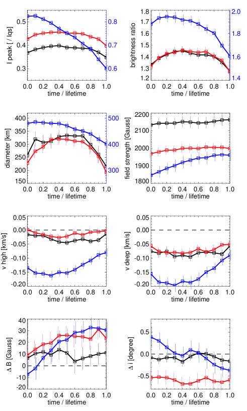
Figure 15.— Temporal evolution of peak brightness ($I_{\rm peak}$), brightness ratio, diameter, field strength, $v_{\rm high}$, $v_{\rm deep}$, $\Delta B$, and $\Delta i$ for central (black), peripheral (red), and grain-origin (blue) UDs. The axis for grain-origin UDs is separately shown to the right in the panels of $I_{\rm peak}$, brightness ratio, and diameter. The standard errors of the mean (SEM) are indicated by the vertical lines.

We have studied the temporal evolution of UDs using the ones that were observed from birth to death and had lifetimes longer than 620 s. In total, 36 central, 50 peripheral, and 66 grain-origin UDs were chosen for this analysis. By normalizing the lifetimes to unity it is possible to average all the evolutionary curves. The results are shown in Figure 15 for eight parameters: peak brightness ($I_{\rm peak}$), brightness ratio, diameter, field strength, $v_{\rm high}$, $v_{\rm deep}$, $\Delta B$, and $\Delta i$. The parameters have been averaged over an area of $7\times 7$ pixels centered at the UD’s position.

Evolution of Central and Peripheral UDs

For central and peripheral UDs, the peak brightness, the brightness ratio, and the diameter show a symmetric increase and decrease over time. The brighter $I_{\rm peak}$ and weaker field strengths observed in peripheral UDs are a natural consequence of their location in the more external parts of the umbra. Both central and peripheral UDs harbor upflows (negative $v_{\rm high}$ and $v_{\rm deep}$) that grow with time, reach a maximum when the UDs are mature, and then decrease more or less symmetrically. The brightness follows a similar pattern. Thus, there is a positive correlation between brightness and upflows, which is a sign of convection.

The field strength and $\Delta B$ are nearly constant, although $\Delta B$ shows a tendency to increase during the evolution of peripheral UDs. $\Delta i$ is around zero for central UDs and negative for peripheral UDs (indicating more vertical fields), with little variations over time.

Evolution of Grain-Origin UDs

For grain-origin UDs, all parameters other than bisector velocities show patterns of monotonic increases or decreases. These patterns are caused by the smooth transition from penumbral grains to circular UDs in the central umbra. The bisector velocities peak shortly after the appearance of the UDs, when the tips of penumbral grains are completely detached. Although with large scatter, locally weaker and more inclined fields are found in the first half of the UD’s lifetime, while opposite properties (locally enhanced and more vertical fields) appear in the latter half.

5.2.4 Scatter Relations

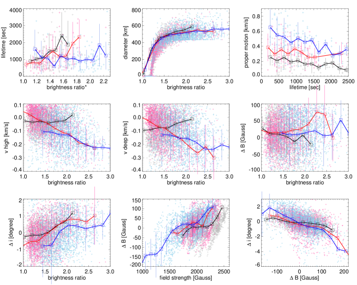
Figure 16.— Scatter plots of brightness ratio, lifetime, proper motion, diameter, field strength, $v_{\rm high}$, $v_{\rm deep}$, $\Delta B$, and $\Delta i$, for central (black), peripheral (red), and grain-origin (blue) UDs. The squares and the thick lines indicate the average values in the corresponding bins. The 1-$\sigma$ fluctuations within the bins are shown by vertical lines. The brightness ratio used in the top left panel is an average over the UD’s lifetime.

Scatter plots of various parameters are displayed in Figure 16, separately for central, peripheral, and grain-origin UDs (black, red, and blue, respectively). In general, all types of UDs exhibit similar relations between parameters, although there are some differences in bisector velocities. Figure 16 shows that:

1. Brighter UDs tend to have longer lifetimes. This is because most of them are recurrent. Other than that, the lifetime is almost constant regardless of the type of UD.

2. The diameter increases linearly for brightness ratios up to 1.4 due to the way it is calculated. For larger ratios the diameter saturates to a constant value of about 500 km, demonstrating that UDs have a typical size.

3. The proper motion speed decreases linearly with lifetime: short-lived UDs move faster.

4. For peripheral and grain-origin UDs, the stronger upflows are found in the brighter structures. Central UDs show the opposite tendency.

5. There is no correlation between $\Delta B$ and brightness ratio.

6. Brighter UDs exhibit more inclined fields than dark UDs, although the inclination difference is not larger than 2^∘ on average.

7. There is a clear correlation between $\Delta B$ and field strength. For UDs with strong fields ($>$2000 G), $\Delta B$ is positive and reaches up to $\approx$100 G.

8. The most inclined fields are associated with negative $\Delta B$ perturbations. UDs with more vertical fields tend to show positive $\Delta B$ values.

Bisector velocities, $\Delta B$, and $\Delta i$ are the most important parameters to decide on the convective nature of UDs. The field-free convection model of UDs suggests upflows, weaker, and more inclined magnetic fields. These conditions are indeed true for relatively weak UDs ($<2000$ G). However, strongly magnetized UDs ($>2000$ G) usually show positive $\Delta B$ perturbations and more vertical field lines. We conjecture that the stronger upflows observed in the darker central UDs may be the result of contamination by molecular lines.

6. Discussion and Conclusion

In this paper we have performed a detailed analysis of UDs in a mature sunspot using data from the CRISP spectropolarimeter. The excellent spatial resolution, temporal cadence, and polarimetric sensitivity of the measurements are ideal for UD studies. The perturbations caused by UDs are usually very small, and thus an statistical approach has to be followed to reveal their common properties. Our work addresses for the first time the temporal evolution of velocity and magnetic fields in and around UDs, using a statistically significant sample of UDs.

Convection in the umbra

UDs are considered to be the manifestation of convection in the presence of the strong umbral field, while more vigorous convection occurs in the quiet Sun in the form of granules. The morphological differences between granules and UDs can be seen in Figure 8. Driven by overshooting cellular convection, granules are characterized by sharp edges and irregular polygonal shapes (Spruit et al., 1990). UDs, on the other hand, show Gaussian brightness profiles. Linear theory reveals that the preferred horizontal scale of convection decreases with increasing field strength (Weiss et al., 1990), which explains why UDs are smaller than granules. The convective origin of UDs seems well established, as many papers including ours found a good correlation between upflows and brightness. However, in the umbra there are other diffuse areas with enhanced brightness whose origin is still unknown. Our speculation that the diffuse bright areas of the umbra are also caused by convection could not be unambiguously confirmed on the basis of a unique relation between brightness and velocities (Figure 9).

Photometric properties

Watanabe et al. (2009a) found constant lifetimes regardless of the UD type and the structure of magnetic field at the position of the UD. This is in agreement with our results (Section 5.2.4). However other studies report longer lifetimes for brighter UDs (Tritschler & Schmidt, 2002; Bharti et al., 2010), and we speculate this is partly due to the fact that bright UDs tend to reoccur at the same position.

A correlation between shorter lifetime and faster proper motion is reported for the first time in this paper (Figure 16). If the energy dissipation rate is proportional to the UD speed, the lifetime can be expected to be reduced for fast-moving UDs, as observed. We also find that the travelled distance depends linearly on lifetime, i.e., long-lived UDs travel longer distances even though they move at lower speeds. The same conclusion can be obtained from a similar analysis of the data set of Watanabe et al. (2009a).

We found UD diameters consistent with the values reported in the literature, i.e., about 400 km on average. The Gaussian shape of the histogram (Figure 4) and the lack of dependence of the diameter on brightness ratio (Figure 16) suggest that UDs indeed have a “typical” size, regardless of their type. This common UD size is probably determined by a universal near-surface stratification in mature sunspots. However, the scatter plot analysis performed in Section 5.2.4 did not reveal any physical parameter having a strong correlation with the UD size.

The intensity oscillations in UDs reported by, e.g., Rimmele (1997) have not been studied in this paper because of the uncertainties that residual seeing fluctuations may introduce. However it is true that many UDs show recurrence, as observed also by Louis et al. (2012). For example, the peripheral UD#C displayed in Figure 22 reappeared twice within a time interval of 13 minutes. This timescale is comparable to the oscillatory period of the UDs shown in Rimmele (1997) and Watanabe et al. (2009b).

Categorization of UDs

We classified the observed UDs in central, peripheral, and grain-origin UDs according to their place of birth. Do these categories represent physically different structures or different manifestations of the same phenomenon? Grain-origin UDs have larger brightness ratios, larger sizes, and faster proper motions than the other UDs. The temporal evolution of grain-origin UDs is smooth and shows monotonic changes, while central and peripheral UDs show mound-shaped evolutionary curves (Figure 15). Despite this, the scatter plots presented in Figure 16 suggest that the properties of grain-origin UDs lie on the extension lines of those of central and peripheral UDs. The differences between them may arise from stronger convection in grain-origin UDs rendered possible by the weaker background field. Spruit & Scharmer (2006) speculated that field-free convection can explain both UDs and penumbral grains. The computer simulations of Heinemann et al. (2007) and Rempel et al. (2009) succeeded in reproducing basic properties of penumbral filaments and UDs as weakly-magnetized convective structures. Our results are in general agreement with the predictions of this scenario, although they also indicate that UDs are far from being completely field-free (at least in the photospheric layers accessible to the observations).

Substructures

Localized downflow patches at the periphery of UDs are considered to be a signature of overturning convection in UDs (Schüssler & Vögler, 2006). In Section 5.1.5 we presented some examples of downflow patches without performing a full statistical analysis. The patches of Figure 11 have sizes of 0$\farcs$2 and redshifts of up to 0.75  km s^-1. Both the size and the velocity are in good agreement with those reported by Ortiz et al. (2010) in a pore. The fact that the downflow patches are observable only at very high bisector levels (i.e., deep photospheric layers) is also consistent with the results of those authors.

However, many UDs do not show downflow patches in our data. This lack of detection could be due to:

1. Insufficient spatial resolution.

2. The existence of downflows only in deep layers that cannot be probed by the Fe I 6301 and 6302 Å lines.

3. The transient nature of the downflows, which could appear only in a particular phase of the UD’s evolution.

4. The possibility that the convective energy escapes to the upper layers instead of returning to deep layers (see the narrow jet-like upflows above the cusp in Schüssler & Vögler, 2006).

The two UDs featured in Figure 11 are in the peak brightness phase when they show downflows. Possibly the speed of the downflows reaches a maximum when the brightness is also maximum.

Velocities in UDs

Upflows and brightness follow similar evolutionary patterns in UDs (Figure 15). This correlation supports the convective nature of UDs (Sobotka & Jurčák, 2009; Watanabe et al., 2010). The scatter plots of velocity vs brightness shown in Figure 16 also point to a convective origin of UDs. For central UDs, however, we observe stronger blueshifts in darker structures, although the tendency is not very pronounced. We suspect this is an artifact caused by systematic blueshifts in very cold umbral areas.

The velocities observed within UDs are likely to represent field-aligned flows, because upflows are readily found on the disk-center side where the field is closer to the line-of-sight direction, compared to the limb side (Section 5.1.4). The same effect can be observed in the Evershed flow (Figure 3), which is also a field-aligned flow.

Magnetic field in and around UDs

The field-free convection model of UDs (Schüssler & Vögler, 2006) predicts weaker and more inclined fields in UDs. Our scatter analysis (Figure 16) confirms these properties, but only for UDs with fields below 2000 G. In strongly magnetized UDs ($>2000$ G), the magnetic field is enhanced and more vertical compared to the surroundings. For grain-origin UDs, the physical conditions also depend on the phase of evolution: in the first half of their lifetime, weaker and more inclined fields appear, while stronger and more vertical fields are observed in the latter half as the UDs intrude into the umbra. To the best of our knowledge, the enhanced and more vertical fields of strongly magnetized UDs cannot be explained by currently available UD models.

We observe strong field regions at the migration front of grain-origin UDs for the first time (see the evolution of UD#D and UD#E in Section 5.1.4). These strong field regions seem to impede the migration of the UDs. The situation is reminiscent of that modeled by Schlichenmaier et al. (1998), where a weakly magnetized penumbral flux tube pushes and compresses the pre-existing vertical field at the leading edge. However, also a weakly magnetized convective structure would produce a compression of the adjacent magnetic field, which has to wrap around the field-free gas. The MHD simulations performed by Heinemann et al. (2007) predict the existence of enhanced field regions surrounding grain-origin UD only in layers deeper than the continuum forming region (see Figure 3 in that paper), but on both the leading and the tail sides. Our observation did not find field enhancements on the tail side.

Final remarks

This work extends our knowledge of the temporal evolution of velocities and magnetic fields in UDs. We found some new and unanswered results that may provide constraints to future modeling efforts. A pioneering comparison of observational and computer-simulated UDs has been performed by Bharti et al. (2010), and this kind of studies should be extended.

At the same time, more spectropolarimetric observations of UDs at high cadence should be performed. The temporal resolution of our data, 63 s, seems appropriate to track the evolution of UDs, but is insufficient for resolving the evolution of UD substructures. UDs will remain one of the most challenging targets for solar observations in the coming years.

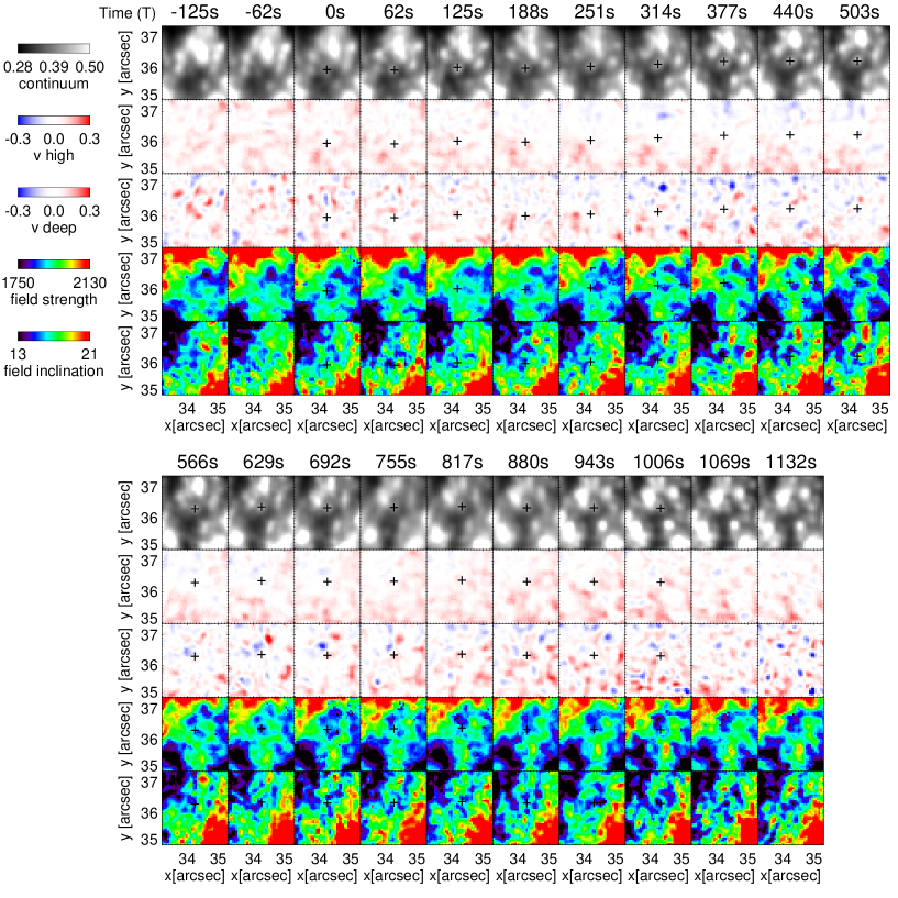
Figure 17.— Temporal evolution of a central UD (#A) from 2 frames before appearance until 2 frames after disappearance. From top to bottom, maps of continuum intensity, $v_{\rm high}$, $v_{\rm deep}$, field strength, and field inclination are shown. $T=0$ s corresponds to the appearance of the UD. The black plus symbols indicate the UD position. The $(x,y)$ coordinates follow the coordinate system used in Figure 1.

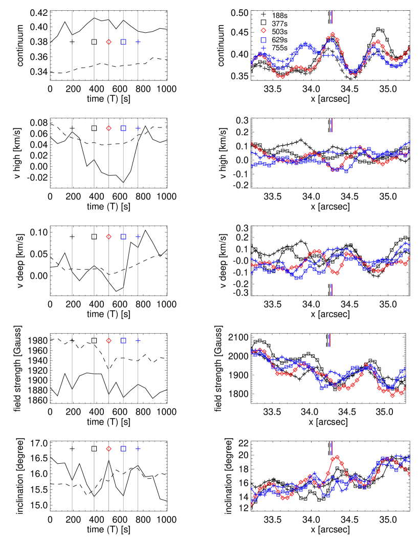
Figure 18.— Left: Temporal variation of continuum intensity, $v_{\rm high}$, $v_{\rm deep}$, field strength, and field inclination for central UD#A (solid line, average within UD’s position $\pm$ 2 pixel area). The dashed lines correspond to the dark background. Time starts from the appearance of the UD. Right: Cuts along the $x$-direction of continuum intensity, $v_{\rm high}$, $v_{\rm deep}$, field strength, and field inclination. The five different lines mark the following times: 188 s (black plus, dashed line), 377 s (black square), 503 s (red diamond), 629 s (blue square), and 755 s (blue plus, dashed line). The short vertical lines at the upper or lower x-axes indicate the UD’s $x$-axis positions in those five instants.

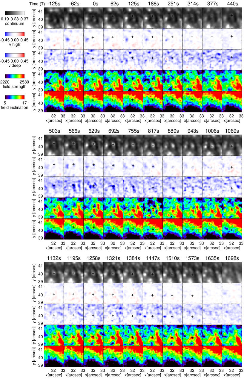
Figure 19.— Same as Figure 17, for central UD#B.

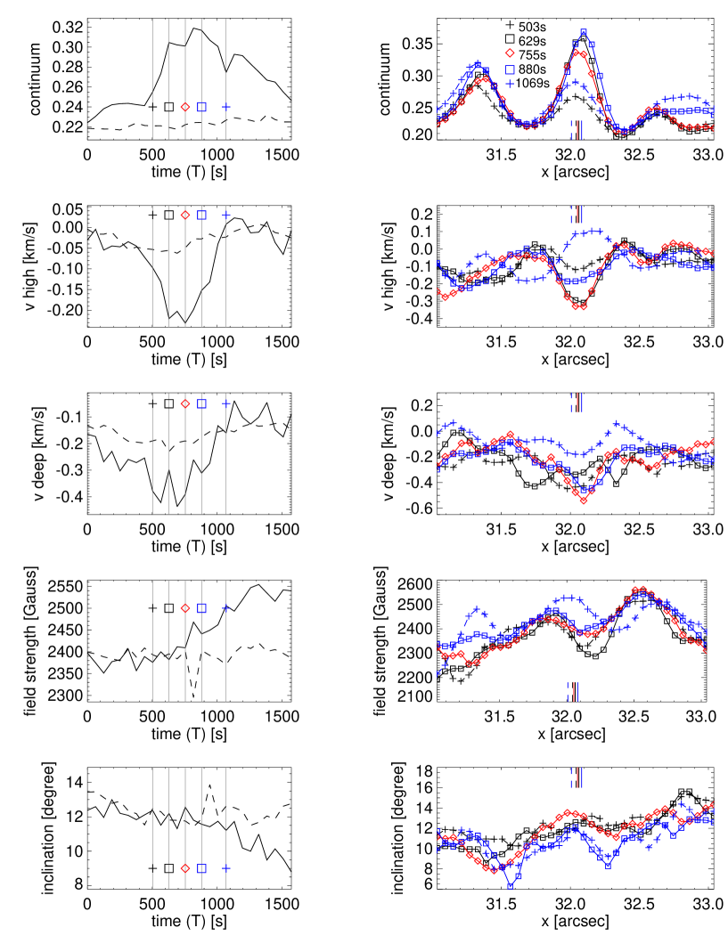
Figure 20.— Same as Figure 18, for central UD# B. The times corresponding to the five different lines in the right panels are 503 s (black plus, dashed line), 629 s (black square), 755 s (red diamond), 880 s (blue square), and 1069 s (blue plus, dashed line).

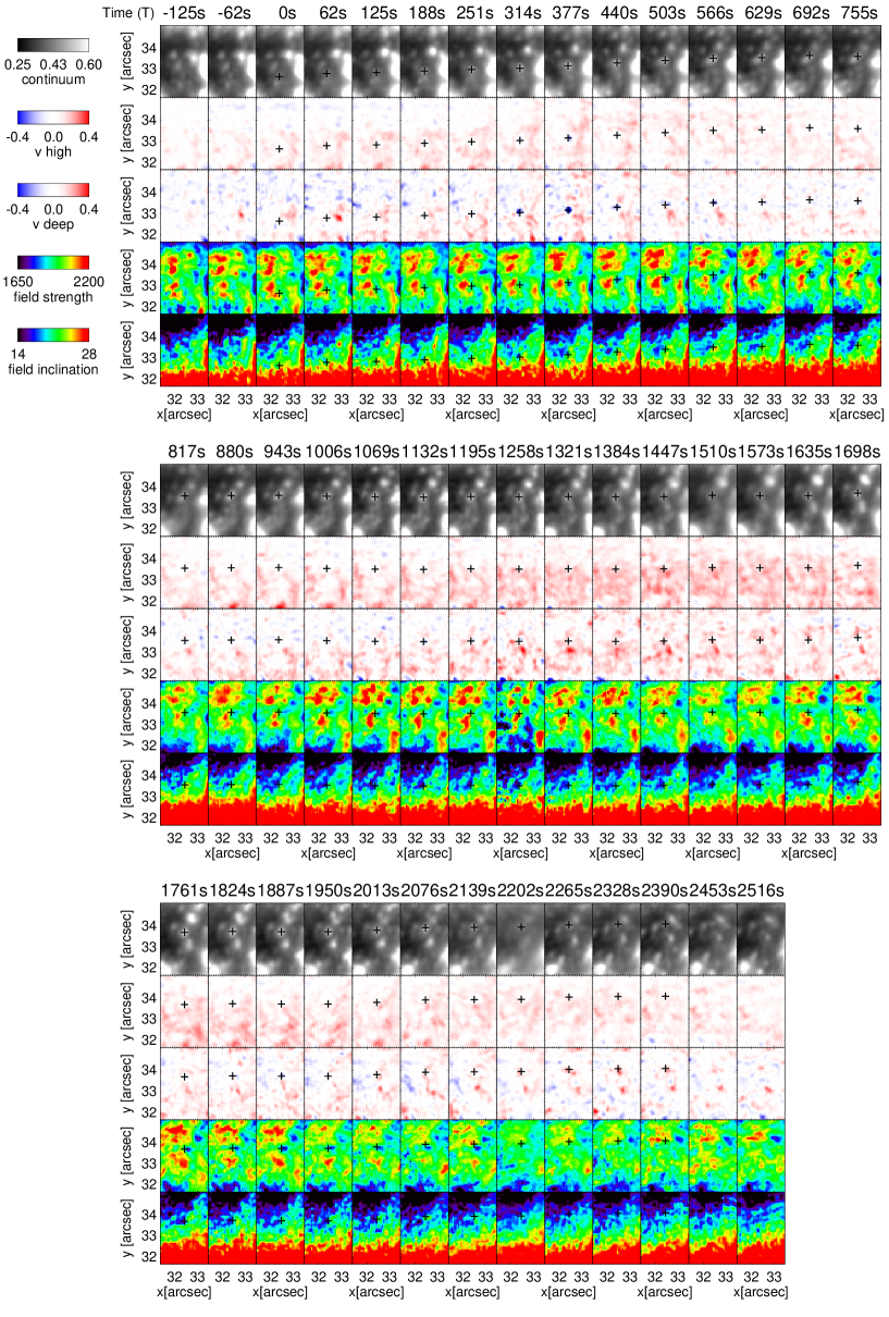
Figure 21.— Same as Figure 17, for peripheral UD#C

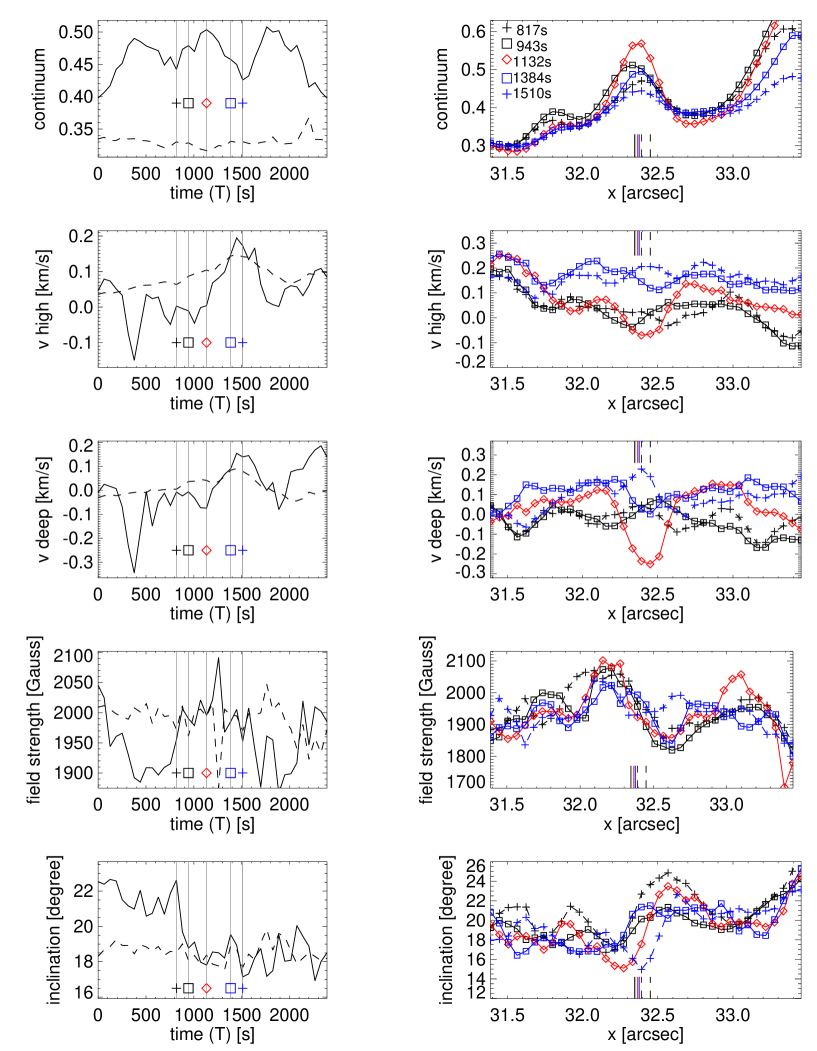
Figure 22.— Same as Figure 18, for peripheral UD#C. The times corresponding to the five different lines in the right panels are 817 s (black plus, dashed line), 943 s (black square), 1132 s (red diamond), 1384 s (blue square), and 1510 s (blue plus, dashed line).

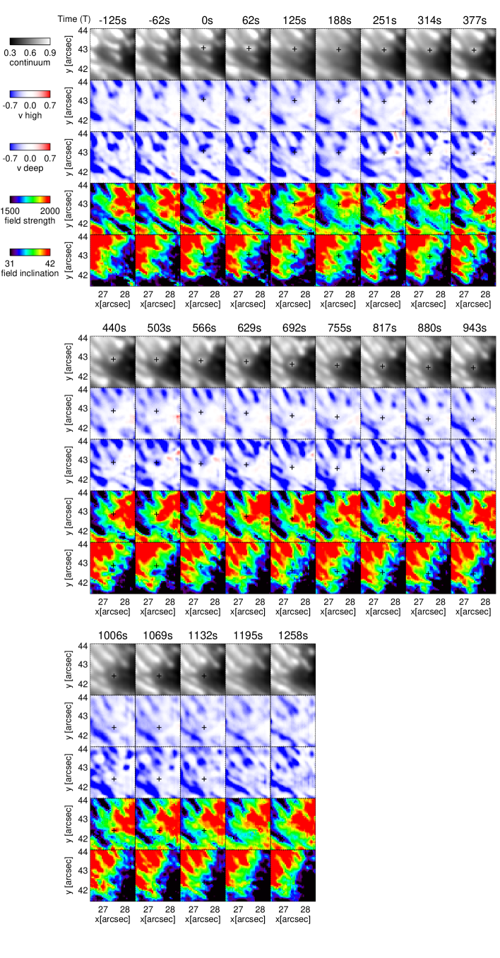
Figure 23.— Same as Figure 17, for grain-origin UD#D

.

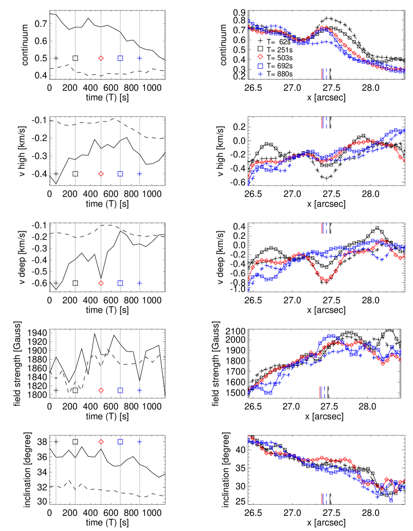
Figure 24.— Same as Figure 18, for grain-origin UD#D. The times corresponding to the five different lines in the right panels are 62 s (black plus, dashed line), 251 s (black square), 503 s (red diamond), 692 s (blue square), and 880 s (blue plus, dashed line).

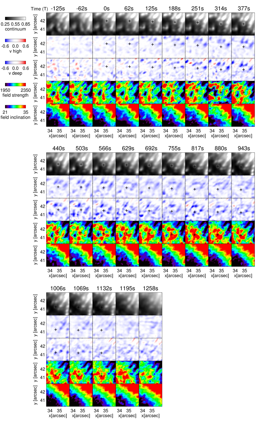
Figure 25.— Same as Figure 17, for grain-origin UD#E.

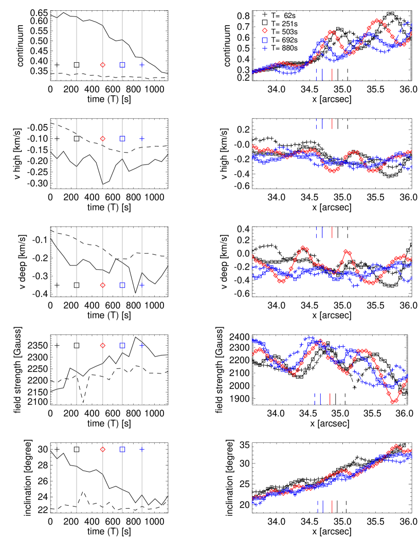
Figure 26.— Same as Figure 18, for grain-origin UD#E. The times corresponding to the five different lines in the right panels are 62 s (black plus, dashed line), 251 s (black square), 503 s (red diamond), 692 s (blue square), and 880 s (blue plus, dashed line).

References

- Alissandrakis et al. (1987) Alissandrakis, C. E., Dialetis, D., & Tsiropoula, G. 1987, A&A, 174, 275
- Bahng & Schwarzschild (1961) Bahng, J., & Schwarzschild, M. 1961, ApJ, 134, 312
- Bharti et al. (2010) Bharti, L., Beeck, B., & Schüssler, M. 2010, A&A, 510, A12+
- Bharti et al. (2007a) Bharti, L., Jain, R., & Jaaffrey, S. N. A. 2007a, ApJ, 665, L79
- Bharti et al. (2007b) Bharti, L., Joshi, C., & Jaaffrey, S. N. A. 2007b, ApJ, 669, L57
- Collados et al. (1994) Collados, M., Martinez Pillet, V., Ruiz Cobo, B., del Toro Iniesta, J. C., & Vazquez, M. 1994, A&A, 291, 622
- Deinzer (1965) Deinzer, W. 1965, ApJ, 141, 548
- Ewell (1992) Ewell, Jr., M. W. 1992, Sol. Phys., 137, 215
- Heinemann et al. (2007) Heinemann, T., Nordlund, Å., Scharmer, G. B., & Spruit, H. C. 2007, ApJ, 669, 1390
- Hirzberger et al. (1999) Hirzberger, J., Bonet, J. A., Vázquez, M., & Hanslmeier, A. 1999, ApJ, 515, 441
- Kitai et al. (2007) Kitai, R., et al. 2007, PASJ, 59, 585
- Louis et al. (2012) Louis, R. E., Mathew, S. K., Bellot Rubio, L. R., Ichimoto, K., Ravindra, B., & Raja Bayanna, A. 2012, ApJ, 752, 109
- Markwardt (2009) Markwardt, C. B. 2009, in Astronomical Society of the Pacific Conference Series, Vol. 411, Astronomical Data Analysis Software and Systems XVIII, ed. D. A. Bohlender, D. Durand, & P. Dowler, 251
- Martínez Pillet & Vázquez (1993) Martínez Pillet, V., & Vázquez, M. 1993, A&A, 270, 494
- Moradi et al. (2010) Moradi, H., et al. 2010, Sol. Phys., 267, 1
- Ortiz et al. (2010) Ortiz, A., Bellot Rubio, L. R., & Rouppe van der Voort, L. 2010, ApJ, 713, 1282
- Rempel et al. (2009) Rempel, M., Schüssler, M., & Knölker, M. 2009, ApJ, 691, 640
- Riethmüller et al. (2008a) Riethmüller, T. L., Solanki, S. K., & Lagg, A. 2008a, ApJ, 678, L157
- Riethmüller et al. (2008b) Riethmüller, T. L., Solanki, S. K., Zakharov, V., & Gandorfer, A. 2008b, A&A, 492, 233
- Rimmele & Marino (2006) Rimmele, T., & Marino, J. 2006, ApJ, 646, 593
- Rimmele (1997) Rimmele, T. R. 1997, ApJ, 490, 458
- Roudier & Muller (1987) Roudier, T., & Muller, R. 1987, Sol. Phys., 107, 11
- Ruiz Cobo & del Toro Iniesta (1992) Ruiz Cobo, B., & del Toro Iniesta, J. C. 1992, ApJ, 398, 375
- Scharmer (2006) Scharmer, G. B. 2006, A&A, 447, 1111
- Scharmer et al. (2003) Scharmer, G. B., Bjelksjo, K., Korhonen, T. K., Lindberg, B., & Petterson, B. 2003, in Presented at the Society of Photo-Optical Instrumentation Engineers (SPIE) Conference, Vol. 4853, Society of Photo-Optical Instrumentation Engineers (SPIE) Conference Series, ed. S. L. Keil & S. V. Avakyan, 341–350
- Schlichenmaier et al. (1998) Schlichenmaier, R., Jahn, K., & Schmidt, H. U. 1998, A&A, 337, 897
- Schnerr et al. (2011) Schnerr, R. S., de La Cruz Rodríguez, J., & van Noort, M. 2011, A&A, 534, A45
- Schüssler & Vögler (2006) Schüssler, M., & Vögler, A. 2006, ApJ, 641, L73
- Selbing (2010) Selbing, J. 2010, ArXiv e-prints
- Sobotka et al. (1993) Sobotka, M., Bonet, J. A., & Vazquez, M. 1993, ApJ, 415, 832
- Sobotka et al. (1997a) Sobotka, M., Brandt, P. N., & Simon, G. W. 1997a, A&A, 328, 682
- Sobotka et al. (1997b) —. 1997b, A&A, 328, 689
- Sobotka et al. (1999a) —. 1999a, A&A, 348, 621
- Sobotka & Jurčák (2009) Sobotka, M., & Jurčák, J. 2009, ApJ, 694, 1080
- Sobotka et al. (1999b) Sobotka, M., Vázquez, M., Bonet, J. A., Hanslmeier, A., & Hirzberger, J. 1999b, ApJ, 511, 436
- Spruit et al. (1990) Spruit, H. C., Nordlund, A., & Title, A. M. 1990, ARA&A, 28, 263
- Spruit & Scharmer (2006) Spruit, H. C., & Scharmer, G. B. 2006, A&A, 447, 343
- Title et al. (1989) Title, A. M., Tarbell, T. D., Topka, K. P., Ferguson, S. H., Shine, R. A., & SOUP Team. 1989, ApJ, 336, 475
- Tritschler et al. (2004) Tritschler, A., Schlichenmaier, R., Bellot Rubio, L. R., the KAOS Team, Berkefeld, T., & Schelenz, T. 2004, A&A, 415, 717
- Tritschler & Schmidt (2002) Tritschler, A., & Schmidt, W. 2002, A&A, 388, 1048
- van Noort et al. (2005) van Noort, M., Rouppe van der Voort, L., & Löfdahl, M. G. 2005, Sol. Phys., 228, 191
- van Noort & Rouppe van der Voort (2008) van Noort, M. J., & Rouppe van der Voort, L. H. M. 2008, A&A, 489, 429
- Watanabe et al. (2009a) Watanabe, H., Kitai, R., & Ichimoto, K. 2009a, ApJ, 702, 1048
- Watanabe et al. (2009b) Watanabe, H., Kitai, R., Ichimoto, K., & Katsukawa, Y. 2009b, PASJ, 61, 193
- Watanabe et al. (2010) Watanabe, H., Tritschler, A., Kitai, R., & Ichimoto, K. 2010, Sol. Phys., 266, 5
- Weiss et al. (1990) Weiss, N. O., Brownjohn, D. P., Hurlburt, N. E., & Proctor, M. R. E. 1990, MNRAS, 245, 434
.