Generalized second law of thermodynamics in the emergent universe for some viable models of $f(T)$ gravity

Abstract

The present work is motivated by the study of reference karmani , where the generalized second law (GSL) of thermodynamics has been investigated for a flat FRW universe for three viable models of $f\left(T\right)$ gravity. We have here considered a non-flat universe and, accordingly, studied the behaviors of equation of state (EoS) parameter $\omega$ and of the deceleration parameter $q$. Subsequently, using the first law of thermodynamics, we derived the expressions for the time derivative of the total entropy of a universe enveloped by apparent horizon. In the next phase, with the choice of scale factor $a\left(t\right)$ pertaining to an emergent universe, we have investigated the sign of the time derivatives of total entropy for the models of $f(T)$ gravity considered.

I Introduction

The cosmic acceleration we are able to see today has been supported by many independent cosmological observational data. The origin of Dark Energy (DE), which is widely believed to be responsible for this cosmic acceleration, is one of the most serious problems in modern cosmology. Nojiri and Odintsov odintsov1 reviewed various modified gravities considered as gravitational alternative for DE. Specifically, they odintsov1 considered the versions of $f(R)$, $f(G)$ or $f(R,G)$ gravity models with non-linear gravitational coupling or string-inspired model with Gauss-Bonnet-dilaton coupling in the late universe where they lead to cosmic speed-up. In another work, Nojiri and Odintsov odintsov2 developed the reconstruction program for the number of modified gravities like scalar-tensor theory, $f(R)$, $f(G)$ and string-inspired, scalar-Gauss-Bonnet gravity. Modified gravity with $\ln R$ or $R^{-n}(\ln R)^{m}$ terms, which grow at small curvature, was discussed by Nojiri and Odintsov odintsov3 . Abdalla et al odintsov4 discussed modified gravity which includes negative and positive powers of curvature and provides gravitational DE: he demonstrated that, in General Relativity plus a term containing a negative power of curvature, cosmic speed-up may be achieved. In a recently published exhaustive review, Nojiri and Odintsov odintsov5 discussed the structure and cosmological properties of a number of modified theories, including traditional $f(R)$ and Horava-Lifshitz $f(R)$ gravity, scalar-tensor theory, string-inspired and Gauss-Bonnet theory, non-local gravity, non-minimally coupled models, and power-counting renormalizable covariant gravity. Motivated by attempts to explain the observed acceleration of the universe in a natural way, there has been a great deal of recent interest in a generalization of this theory in which the Lagrangian is an arbitrary algebraic function $f$ of the Lagrangian of teleparallel gravity $T$ Li . This is similar to creating $f(R)$ gravity theories that are a generalization of general relativity (a review on $f(R)$ gravity is available in Sotiriou ). This gravity is dubbed as $f(T)$ gravity. Review on $f(T)$ gravity is available in references Zheng ; Dent ; Bengochea ; Myrza ; cai . This gravity describes the present accelerating expansion of the universe without resorting to dark energy. It is a generalization of the teleparallel gravity (TG) by replacing the so-called torsion scalar $T$ with $f(T)$ karmani . In Chattopadhyay , the EoS parameter was reconstructed for emergent universe under $f(T)$ gravity. Bamba and Geng bambageng explored thermodynamics of the apparent horizon in $f(T)$ gravity with both equilibrium and non-equilibrium descriptions. In another work, Bamba et al bambaetal studied the cosmological evolutions of the EoS for DE in the exponential and logarithmic (as well as their combination) $f(T)$ theories. In a recent work, Bamba et al bambaetal1 reconstructed a model of $f(T)$ gravity with realizing the finite-time future singularities. In addition, they bambaetal1 have explicitly shown that a power-law-type correction term $T^{\beta}$ (with $\beta>1$) such as a $T^{2}$ term can remove the finite-time future singularities in $f(T)$ gravity.
The possibilities of an emergent universe Ellis1 ; Ellis2 ; Paul have been studied recently in a number of papers in which one looks for an ever-existing and large enough universe so that the space-time may be treated as classical entities. In these models, the universe in the infinite past is in an almost static state but it eventually evolves into an inflationary stage Paul . An emergent universe model can be defined as a singularity free universe which is ever existing with an almost static nature in the infinite past $(t\rightarrow-\infty)$ and then evolves into an inflationary stage Debnath . In references Paul ; Canadian ; Chattopadhyay the characteristics of an emergent universe have been summarized as:

1. the universe is almost static at the finite past $(t\rightarrow-\infty)$ and isotropic and homogeneous at large scales;

2. it is ever existing and there is no timelike singularity;

3. the universe is always large enough so that the classical description of space-time is adequate;

4. the universe may contain exotic matter so that the energy conditions may be violated;

5. the universe is accelerating as suggested by recent measurements of distances of high redshift type Ia supernovae.

Chattopadhyay and Debnath Canadian considered the generalized Ricci DE and generalized holographic DE (HDE) in the scenario of an emergent universe and they studied the behaviors of the potential and the chameleon scalar fields. In references Debnath ; Canadian ; Chattopadhyay , the choice of scale factor $a\left(t\right)$ for emergent universe was $a\left(t\right)=a_{0}\left(\eta+e^{Bt}\right)^{n}$, where $a_{0}$, $\eta$, $B$ and $n$ are positive constants.

Brevik et al odintsov5 studied the entropy of a FRW universe filled with dark energy (cosmological constant, quintessence, or phantom). Bamba et al bambaodintsov discussed the relation between the expression of the entropy and the contribution from the modified gravity as well as the matter to the definition of the energy flux (heat).

The present work is motivated by the work of karmani , who investigated the validity of the generalized second law (GSL) of gravitational thermodynamics in the framework of $f(T)$ gravity. The present study deviates the earlier work in the following aspects: (i) we have considered three viable models of $f(T)$ gravity without the assumption of flat universe and examined the cases of non-flat universe; (ii) we have examined the validity of GSL of thermodynamics for a particular choice of scale factor pertaining to emergent universe; (iii) we have investigated some particular cases for the violation of GSL.

II $f(T)$ gravity in non-flat universe

In the framework of $f(T)$ theory, the action $I$ of modified TG is given by karmani :

$$I=\frac{1}{16\pi G}\int d^{4}x\sqrt{-g}\left[f(T)+L_{m}\right]$$ (1)

where $L_{m}$ is the Lagrangian density of the matter inside the universe. We consider a Friedmann-Robertson-Walker (FRW) universe filled with the pressureless matter (i.e., $p_{m}=0$). Choosing $(8\pi G=1)$ the modified Friedman equations in the framework of $f(T)$ gravity are given by karmani ; Ferraro :

$$H^{2}+\frac{k}{a^{2}} = \frac{1}{3}\left(\rho_{m}+\rho_{T}\right),$$ (2)

$$\dot{H}-\frac{k}{a^{2}} = -\frac{1}{2}\left(\rho_{m}+\rho_{T}+p_{T}\right),$$ (3)

where:

$$\rho_{T} = \frac{1}{2}(2Tf_{T}-f-T),$$ (4)

$$p_{T} = -\frac{1}{2}\left[-8\dot{H}Tf_{TT}+(2T-4\dot{H})f_{T}-f+4\dot{H}-T\right].$$ (5)

The torsion scalar $T$ is defined, for non-flat universe, as Ferraro :

$$T=-6\left(H^{2}+\frac{k}{a^{2}}\right),$$ (6)

In above Equations, $k$ is the curvature parameter, which can assume the values $\left(-1,0,+1\right)$, $H=\frac{\dot{a}}{a}$ is the Hubble parameter, $\dot{H}$ is the derivative with respect to the cosmic time $t$ of the Hubble parameter $H$, $f_{T}$ is the first derivatie of $f$ with respect to $T$, $f_{TT}$ if the second derivative of $f$ with respect to $T$ and $\rho_{m}$ is the energy density of the matter. Moreover, $\rho_{T}$ and $p_{T}$ are the torsion contributions to the energy density and pressure. Energy conservation equations are given by:

$$\dot{\rho}_{m}+3H\rho_{m}=0,\\ \dot{\rho}_{T}+3H(\rho_{T}+p_{T})=0.$$

The effective EoS parameter due to the torsion contribution is defined as karmani :

$$\omega_{T}=-1-\frac{\dot{T}}{3H}\left(\frac{2Tf_{TT}+f_{T}-1}{2Tf_{T}-f-T}\right).$$ (7)

From Eqs. (2), (4) and (6) we get $\rho_{m}$ as:

$$\rho_{m}=\frac{1}{2}\left(f-2Tf_{T}\right).$$ (8)

Using Eqs. (3) and (9), we derive that the time derivative of Hubble parameter $H$ is given by:

$$\dot{H}=-\frac{1}{2}\left(\frac{\rho_{m}-\frac{2k}{a^{2}}}{f_{T}+2Tf_{TT}}\right).$$ (9)

Using Eqs. (6) and (10), we derive the following expression for $\dot{T}$:

$$\dot{T}=\frac{12H}{f_{T}+2Tf_{TT}}\left[\frac{k(f_{T}+2Tf_{TT}-1)}{a^{2}}+\frac{\rho_{m}}{2}\right].$$ (10)

The deceleration parameter $q$ can be obtained from Eqs. (2), (9) and (10) as follow:

$$q=-1-\frac{\dot{H}}{H^{2}}=-1+\frac{3}{2}\left\{\frac{\rho_{m}a^{2}-2k}{\left(f_{T}+2Tf_{TT}\right)\left[a^{2}\left(\rho_{m}+\rho_{T}\right)-3k\right]}\right\}.$$ (11)

III GSL in $f(T)$ gravity

The apparent horizon has been argued as a causal horizon for a dynamical spacetime and it is associated with gravitational entropy and surface gravity Bak . The radius of the apparent horizon, which is denoted by $R_{A}$, is given by sheykhi :

$$R_{A}=\frac{1}{\sqrt{H^{2}+\frac{k}{a^{2}}}}.$$ (12)

In the present work, we are investigating the validity of GSL in a non-flat FRW universe filled with pressureless Dark Matter (DM). The GSL can be expressed as $\dot{S}_{A}+\dot{S}_{m}\geq 0$, where $S_{A}$ denotes the Bekenstein-Hawking entropy on the horizon and $S_{m}$ is the entropy due to the matter sources inside the horizon akbar . Detailed account of the GSL is available in sheykhi ; jamil ; paddy . From the first law of thermodynamics one can get (Clausius relation) $-dE=T_{A}dS_{A}$ to the apparent horizon $R_{A}$. The Friedmann equation in the Einstein gravity can be derived if we take the Hawking temperature $T_{A}=1/2\pi R_{A}$ and the entropy $S_{A}=A/4G$ on the apparent horizon, where $A$ is the area of the horizon karmani . However, this definition is changed for other modified gravity theories. In $f(T)$ gravity, it was shown that when $f_{TT}$ is small, the first law of black hole thermodynamics is satisfied approximatively and the entropy of horizon is $S_{A}=\frac{Af_{T}}{4G}$ karmani . In the present work we assume that the boundary of the universe to be enclosed by the dynamical apparent horizon $R_{A}$ and the Hawking temperature on the apparent horizon is given by karmani ; sheykhi :

$$T_{A}=\frac{1}{2\pi R_{A}}\left(1-\frac{\dot{R}_{A}}{2HR_{A}}\right).$$ (13)

Based on the discussions in the previous Section, we compute:

$$T_{A}\dot{S}_{m} = 2\pi R_{A}^{2}(f-2Tf_{T})(\dot{R}_{A}-HR_{A}),$$ (14)

$$T_{A}\dot{S}_{A} = 4\pi\left(1-\frac{\dot{R}_{A}}{2HR_{A}}\right)\left[2\dot{R}_{A}f_{T}+6H\left(\frac{\rho_{m}-\frac{2k}{a^{2}}}{f_{T}+2Tf_{TT}}\right)R_{A}f_{TT}\right],$$ (15)

where $\dot{S}_{m}$ and $\dot{S}_{A}$ denote, respectively, the time derivatives of the entropy due to the matter sources inside the horizon and on the horizon. In the following subsections, we investigate whether $\dot{S}_{m}+\dot{S}_{A}\geq 0$ for three viable choices of $f(T)$ models with the choice of scale factor for emergent scenario, i.e. $a=a_{0}\left(\eta+e^{Bt}\right)^{n}$. The $f(T)$ models considered here are:

1. $f(T)=\gamma T+\lambda T^{m}$, where $\gamma$, $\lambda$ and $m$ are constants Chattopadhyay

2. $f(T)=T-\lambda T\left[1-e^{\left(\beta\frac{T_{0}}{T}\right)}\right]$ where $\lambda=\frac{1-8\pi\frac{\rho_{m0}}{3H_{0}^{2}}}{1-(1-2\beta)e^{\beta}}$karmani

3. $f(T)=T+\lambda(-T)^{n_{1}}$ where $\lambda=\left(\frac{1-8\pi\frac{\rho_{m0}}{3H_{0}^{2}}}{2n_{1}-1}\right)(6H_{0}^{2})^{(1-n_{1})}$ and $n_{1}$ is a constant karmani

$T_{0}$, $\rho_{m0}$ and $H_{0}$ are, respectively, the present values of $T$, energy density of DM and Hubble parameter.

III.1 Model I

First, we consider the model $f(T)=\gamma T+\lambda T^{m}$. In this case, we have that $\dot{T}$ is given by:

$$\dot{T}=\frac{\xi_{1}}{\xi_{2}},$$ (16)

where:

$$\begin{array}[]{c}\xi_{1}=6Be^{Bt}n(e^{Bt}+\eta)^{-3-2n}\left[6(k^{2}(2+\gamma)(e^{Bt}+\eta)^{4}+3a_{0}^{4}B^{4}e^{4Bt}n^{4}\gamma\times\right.\\ \left.(e^{Bt}+\eta)^{4n}-2a_{0}^{2}B^{2}e^{2Bt}kn^{2}(1+2\gamma)(e^{Bt}+\eta)^{2+2n})+a_{0}^{2}(e^{Bt}+\eta)^{2n}\times\right.\\ \left.\left\{-\frac{B^{2}e^{2Bt}n^{2}}{(e^{Bt}+\eta)^{2}}+\frac{k(e^{Bt}+\eta)^{-2n}}{a_{0}^{2}}\right\}^{m}(-6^{m}k(3+4(-2+m)m)(e^{Bt}+\eta)^{4}+3a_{0}^{2}B^{2}e^{2Bt})\lambda\right],\\ \end{array}$$ (17)

$$\begin{array}[]{c}\xi_{2}=a_{0}^{2}\left[-6k\gamma(e^{Bt}+\eta)^{2}+6a_{0}^{2}B^{2}e^{2Bt}n^{2}\gamma(e^{Bt}+\eta)^{2n}+a_{0}^{2}m(6^{m}-2^{1+m}3^{m}m)(e^{Bt}+\eta)^{2+2n}\lambda\times\right.\\ \left.\left\{-\frac{B^{2}e^{2Bt}n^{2}}{(e^{Bt}+\eta)^{2}}+\frac{k(e^{Bt}+\eta)^{-2n}}{a_{0}^{2}}\right\}^{m}\right].\\ \end{array}$$ (18)

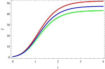
Figure 1: Evolution of $\dot{T}$ with cosmic time $t$ for model I.

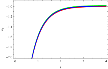
Figure 2: Behavior of $\omega_{T}$ for model I.

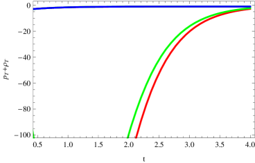
Figure 3: Behavior of $p_{T}+\rho_{T}$ for model I.

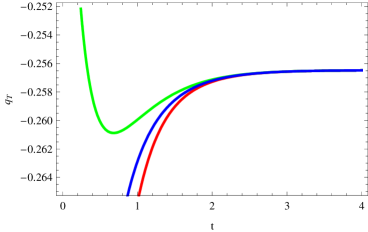
Figure 4: Behavior of $q_{T}$ for model I.

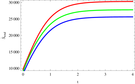
Figure 5: Behavior of $\dot{S}_{total}$ when the apparent horizon is considered as the enveloping horizon under $f(T)=\gamma T+\lambda T^{m}$ i.e. model I.

In Figure 1, we plotted the behavior of $\dot{T}$ for model I and it is found that $\dot{T}$ is an increasing function of the time $t$. The EoS parameter for this model has been plotted in Figure 2, where it is observed that $\omega_{T}\leq-1$, which indicates phantom-like behavior. Moveover, it is observed that from early to late stage of the universe the EoS parameter is tending towards $-1$. This holds for $k=-1,~{}+1$ and $0$. The deceleration parameter $q$, plotted in Figure 3, remains negative throughout the evolution of the universe. This indicates ever-accelerating universe. For all of the above Figures, we have considered the following values for the involved parameters: $B=2,~{}a_{0}=1.5,~{}n=1.2,~{}\eta=3,~{}\gamma=4.02,~{}\lambda=4.03$ and $m=2$. The sum of the pressure $p_{T}$ and the energy density $\rho_{T}$ is plotted in Figure 4, where we can see that $\rho_{T}+p_{T}$ is always negative, indicating the violation of the strong energy condition. In Figure 5, we plotted the time derivative of total entropy $\dot{S}_{total}$ against cosmic time $t$. $\dot{S}_{total}$ is computed using Eqs. (15) and (16), where $f(T)$ has been replaced by the form of model I. $\dot{S}_{total}$ is found to be positive throughout the evolution of the universe, which indicates that the GSL is satisfied by model I under emergent scenario of the universe.

III.2 Model II

In this Section, we consider the model II, given by $f(T)=T-\lambda T\left[1-e^{\left(\beta\frac{T_{0}}{T}\right)}\right]$. The expression of $\dot{T}$ for this model is not reported here since it would occupy too many space. $\dot{T}$ is plotted against cosmic time $t$ in Figure 1: it is observed a behavior similar to that for model I. It may be noted that for model II, our choices for the parameters are $a_{0}=20,~{}B=4,~{}n=0.04$ and $\eta=3$ that satisfy the conditions for emergent universe. Moreover, we choose $\lambda=0.03,~{}\beta=-0.02,~{}\rho_{m0}=0.23$ and $H_{0}=74.2$. In all Figures for this model, the red, green and blue lines correspond to the cases $k=-1$, $k=+1$ and $k=0$, respectively.

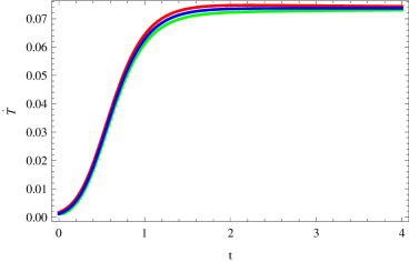
Figure 6: Behavior of $\dot{T}$ for model II.

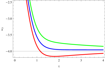
Figure 7: Behavior of $\omega_{T}$ for model II.

Like model I, $\dot{T}$ (plotted in Figure 6) stays positive and exhibits upward movement with evolution of the universe. The EoS parameter $\omega_{T}$, as seen in Figure 7, stays below $-1$ and it never tend to $-1$. This indicates the phantom-like behavior of $\omega_{T}$.

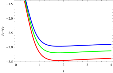
Figure 8: Behavior of $(p_{T}+\rho_{T})$ for model II.

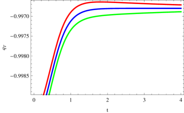
Figure 9: Behavior of $q_{T}$ for model II.

In Figure 8, $(p_{T}+\rho_{T})$ is plotted against $t$: it shows the violation of strong energy condition by model II. The accelerated universe under model II is understandable from Figure 9 which shows that $q_{T}$ is always negative for every choice of the curvature parameter $k$.

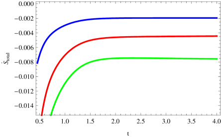
Figure 10: Behavior of $\dot{S}_{total}$ when the apparent horizon is considered as the enveloping horizon under $f(T)=T-\lambda T\left[1-e^{\left(\beta\frac{T_{0}}{T}\right)}\right]$, i.e. model II.

Finally, when we consider the time derivative of total entropy $\dot{S}$ in Figure 10, we find that it remains negative for every choice of $k$. This indicates violation of GSL by model II.

III.3 Model III

In this Section we consider model III where $f(T)=T+\lambda(-T)^{n_{1}}$, where $\lambda=\left(\frac{1-8\pi\frac{\rho_{m0}}{3H_{0}^{2}}}{2n_{1}-1}\right)(6H_{0}^{2})^{(1-n_{1})}$. In order to study the model III, we have taken both $n_{1}<1~{}(n_{1}=\frac{1}{3})$ and $n_{1}>1~{}(n_{1}=1.2)$ into account. The expression of $\dot{T}$ for this model is not reported here since it would occupy too many space. We have plotted $\dot{T}$ in Figure 11, where $\dot{T}$ is found to behave similarly to the cases corresponding to the models I and II.

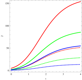
Figure 11: Behavior of $\dot{T}$ for model III i.e. $f(T)=T+\lambda(-T)^{n_{1}}$. The solid lines pertain to $n_{1}<1$ and the dashed lines pertain to $n_{1}>1$.

From Figures 12 and 13, we find that the EoS parameter $\omega_{T}$ has a phantom-like behavior and it tends to $-1$ in both cases, irrespective of the choice of the curvature parameter $k$.

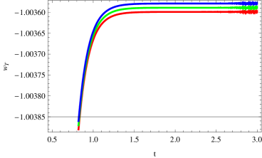
Figure 12: Behavior of $\omega_{T}$ for model III with $n_{1}<1$.

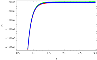
Figure 13: Behavior of $\omega_{T}$ for model III with $n_{1}>1$.

The deceleration parameter $q$, plotted in Figures 14 and 15 for the two different values of $n_{1}$, indicates the realization of the accelerated expansion of the universe for model III forboth $n_{1}<1$ and $n_{1}>1$.

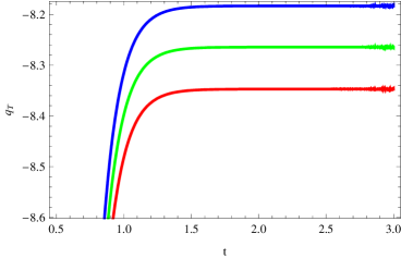
Figure 14: Behavior of $q_{T}$ for model III with $n_{1}<1$.

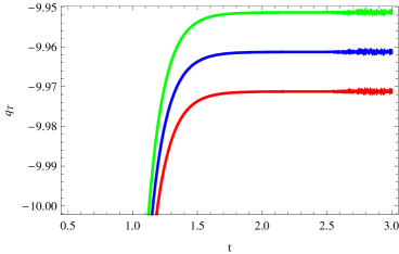
Figure 15: Behavior of $q_{T}$ for model III with $n_{1}>1$.

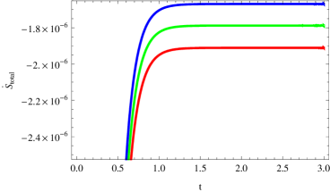
Figure 16: Behavior of $\dot{S}_{total}$ when the apparent horizon is considered as the enveloping horizon under $f(T)=T+\lambda(-T)^{n_{1}}$ with $n_{1}<1$.

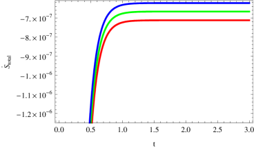
Figure 17: Behavior of $\dot{S}_{total}$ when the apparent horizon is considered as the enveloping horizon under $f(T)=T+\lambda(-T)^{n_{1}}$ with $n_{1}>1$.

Finally, when we plot $\dot{S}_{total}$ in Figures 16 and 17 for the case of model III with apparent horizon as the enveloping horizon, we observe violation of the GSL by model III irrespective of the choices of $n_{1}$.

IV Discussion

In this work, we have considered three viable $f(T)$ gravity with scale factor $a$ pertaining to emergent universe. We have investigated the validity of GSL for all the cases along with some related characteristics. It is observed that for model I, $\dot{T}$ exhibits an increasing pattern in the positive side with evolution of the universe. When we considered the EoS parameter $\omega_{T}$ for this model, we found that, with evolution of the universe, $\omega_{T}$ remains below -1 at earlier stages and tends to -1 at later stage, indicating a phantom-like behavior of $\omega_{T}$. As displayed in Figure 2. In Figure 3 we plotted $\left(p_{T}+\rho_{T}\right)$ against the cosmic time $t$ and we found that it stays at negative level. This indicates violation of strong energy condition. The deceleration parameter $q_{T}$ for this model is plotted against cosmic time $t$ in Figure 4: we found that it is negative throughout. This indicates accelerated phase of the universe. The time derivative of total entropy is plotted in Figure 5 and we find that it remains positive through the evolution of the universe irrespective of the value of $k$. Therefore our observations are that for model I are: (i) the EoS exhibits phantom-like behavior, (ii) the strong energy condition is violated, (iii) we get an accelerating universe and (iv) the GSL of thermodynamics holds irrespective of the curvature of the universe. It should be stated that the apparent horizon has been considered as the enveloping horizon of the universe. Now we consider the model II with the choices of scale factor and enveloping horizon similar to that of model I. All the quantities considered for model I are also considered for model II. From Figure 6, we observe that the behavior of $\dot{T}$ is similar to that of model I. However the EoS parameter $\omega_{T}$, as plotted in Figure 7, exhibits a small difference with model I. In the present case, the EoS parameter $\omega_{T}$ exhibits phantom-like behavior. However, it tends to -1 at later stages of the universe. The strong energy condition is violated like in model I (Figure 8). Moreover, like in model I, we also find an ever accelerating universe (see Figure 9). Finally, when we consider the GSL, we find a prominent difference between model I and model II. In model II, the time derivative of total entropy remains negative through the evolution of the universe. This indicates the violation the GSL. This is displayed in Figure 10. Therefore for model II the observations are following: (i) the EoS exhibits phantom-like behavior, (ii) The strong energy condition is violated, (iii) we get accelerating universe and (iv) generalized second law of thermodynamics is violated here. Here also the above results hold irrespective of the choice of $k$. Now we come to Model III. For model III we have same choices of scale factor and enveloping horizon. However, while considering model III we consider two cases, namely $n_{1}<1$ and $n_{1}>1$. From Figure 11 we find that the time derivative of $T$ remains positive for $n_{1}<1$ as well as $n_{1}>1$ and, in both cases, it shows increasing pattern. In Figure 12 we have plotted EoS parameter for $n_{1}<1$ and we have observed that it is always staying below $-1$ irrespective of the choice of curvature. This indicates phantom-like behavior of the EoS parameter for $n_{1}<1$. In Figure 13, we plot the EoS parameter for $n_{1}>1$ and here also we observe phantom like behavior. In Figure 14 and 15 we plot the deceleration parameter $q_{T}$ for $n_{1}<1$ and $n_{1}>1$: in both cases, we get a negative deceleration parameter $q$, indicating ever accelerating universe. The GSL for $n_{1}<1$ is considered in Figure 16 and we observe that the time derivative of total entropy is staying at negative level, which means a violation of the GSL. The case corresponding to $n_{1}>1$ is considered in Figure 17. Here, we also find that the time derivative of the total entropy is negative through the universe. Therefore, we conclude that the GSL is not valid in this case. The above results hold for $k=-1,~{}+1$ and $0$. Therefore, our observations are the following: (i) the EoS parameter has a phantom-like behavior, (ii) the accelerated expansion of the universe is realized and (iii) the generalized second law of thermodynamics does not work here. The above results are independent of the choice of the curvature parameter $k$.

V Acknowledgements

The first author wishes to thank the Inter-University Centre for Astronomy and Astrophysics (IUCAA), Pune, India for providing warm hospitality during a scientific visit in January 2012, when part of the work was carried out. The third author sincerely acknowledges the Visiting Associateship provided by IUCAA, Pune, India for the period of August 2011 to July 2014 to carry out research in General Relativity and Cosmology. The third author acknowledges the research grant under Fast Track Programme for Young Scientists provided by the Department of Science and Technology (DST), Govt of India. The project number is SR/FTP/PS-167/2011.

References

- (1) K. Karami and A. Abdolmaleki, J. Cosmol. Astropart. Phys. 04 (2012) 007.
- (2) S. Nojiri and S. D. Odintsov, International Journal of Geometric Methods in Modern Physics 4 (2007) 115.
- (3) S. Nojiri and S. D. Odintsov, J. Phys.: Conf. Ser. 66 (2007) 012005 doi:10.1088/1742-6596/66/1/012005.
- (4) S. Nojiri and S. D. Odintsov, General Relativity and Gravitation 36 (2004) 1765.
- (5) M. C. B. Abdalla, S. Nojiri and S. D. Odintsov, Class. Quantum Grav. 22 (2005) L35 doi:10.1088/0264-9381/22/5/L01.
- (6) S. Nojiri and S. D. Odintsov, Physics Reports 505 (2011) 59.
- (7) B. Li, T. P. Sotiriou and J. D. Barrow, Phys. Rev. D 83 (2011) 064035.
- (8) T. P. Sotiriou and V. Faraoni, Rev. Mod. Phys. 82 (2010) 451.
- (9) R. Zheng and Q-G. Huang, J. Cosmol. Astropart. Phys. 03 (2011) 002.
- (10) J. B. Dent, S. Dutta and E. N. Saridakis, J. Cosmol. Astropart. Phys. 01 (2011) 009.
- (11) G. R. Bengochea, Phys. Lett. B 695 (2011) 405.
- (12) R. Myrzakulov, Eur. Phys. J. C 71 (2011) 1752.
- (13) Y-F. Cai, S-H. Chen, J. B. Dent, S. Dutta and E. N. Saridakis, Class. Quantum Grav. 28 (2011) 215011.
- (14) G. F. R. Ellis and R. Maartens, Class. Quantum Grav. 21 (2004) 223.
- (15) G. F. R. Ellis, J. Murugan and C. G. Tsagas, Class. Quantum Grav. 21 (2004) 233.
- (16) S. Mukherjee, B. C. Paul, N. K. Dadhich, S. D. Maharaj and A. Beesham, Class. Quantum Grav. 23 (2006) 6927.
- (17) U. Debnath, Class. Quantum Grav. 25 (2008) 205019.
- (18) S. Chattopadhyay and U. Debnath, Can. J. Phys. 89 (2011) 941.
- (19) I. Brevik, S. Nojiri, S. D. Odintsov and L. Vanzo, Physical Review D, 70 (2004) 043520.
- (20) K. Bamba, C-Q. Geng, S. Nojiri and S. D. Odintsov, EPL 89 (2010) 50003 doi:10.1209/0295-5075/89/50003.
- (21) S. Chattopadhyay and U. Debnath, Int. J. Mod. Phys. D 20 (2011) 1135.
- (22) K. Bamba and C-Q. Geng, J. Cosmol. Astropart. Phys. 11 (2011) 008 doi:10.1088/1475-7516/2011/11/008.
- (23) K. Bamba et al, J. Cosmol. Astropart. Phys. 01(2011)021 doi:10.1088/1475-7516/2011/01/021.
- (24) K. Bamba, R. Myrzakulov, S. Nojiri and S. D. Odintsov, Phys. Rev. D 85 (2012) 104036.
- (25) R. Ferraro and F. Fiorini, Phys. Lett. B 702 (2011) 75.
- (26) D. Bak and S. J. Rey, Class. Quantum Grav. 17 (2000) L83.
- (27) A. Sheykhi Class. Quantum Grav. 27 (2010) 025007.
- (28) M. Akbar Chin. Phys. Lett. 25 (2008) 4199.
- (29) M. Jamil, E. N. Saridakis and M. R. Setare, J. Cosmol. Astropart. Phys. 11 (2010) 032.
- (30) T. Padmanabhan, Reports on Progress in Physics, 73 (2010) 046901