Spherically symmetric gravity coupled to a scalar field with a local Hamiltonian: the complete initial-boundary value problem using metric variables

Abstract

We discuss a gauge fixing of gravity coupled to a scalar field in spherical symmetry such that the Hamiltonian is an integral over space of a local density. In a previous paper we had presented it using Ashtekar’s new variables. Here we study it in metric variables. We specify completely the initial-boundary value problem for ingoing Gaussian pulses.

I Introduction

Spherically symmetric gravity coupled to a scalar field is a rich model, where one can test scenarios of black hole formation, the critical phenomena discovered by Choptuik and Hawking evaporation at the quantum level. For many years the full quantization of the model resisted analysis, in part due to the complicated nature of the Hamiltonian structure of the system. Initial attempts to study the problem were done by Berger, Chitre, Nutku and Moncrief bcnm and further developed by Unruh unruh . The resulting complicated nature of the gauge fixed Hamiltonian led led Unruh to say “I present it here in the hope that someone else may be able to do something with it.” More recently, Husain and Winkler and Daghigh, Kunstatter and Gegenberg huwi , using Painlevé–Gullstrand coordinates simplified somewhat Unruh’s treatment. None of these efforts provided a Hamiltonian that was the spatial integral of a local density, leading to non-local equations of motion with the ensuing difficulty at the time of quantization.

We recently noted that using Ashtekar’s new variables the construction of a local Hamiltonian was possible. It was later suggested by Unruh unruhpersonal and Gegenberg and Kunstatter geku that a similar construction was possible in metric variables. In hindsight, this is not too surprising. The key element used in our construction was that in Ashtekar’s variables the gravitational part of the Hamiltonian constraint becomes the total derivative of a quantity with respect to the radial variable. It turns out that some years ago, Kuchař kuchar introduced canonical coordinates for spherically symmetric vacuum gravity in which one of the coordinates is the mass as function of the radius. The gravitational part of the Hamiltonian constraint in that case is given by the total derivative of the mass with respect to the radial variable. Therefore a construction similar to the one we had carried out with Ashtekar’s variables can be carried out with Kuchař’s variables. We will detail the construction here. As most gauge fixings, only certain families of initial data can be accommodated with a given choice of gauge. We set up a suitable initial-boundary value problem in the gauge fixed theory and for the physically important case of Gaussian pulses.

The organization of this paper is as follows. In section II we discuss the gauge fixing in terms of Kuchař’s variables. In section III we set up the Hamiltonian. In section IV we study the initial-boundary value problem, in particular for Gaussian pulses. We end with a discussion of possibilities for quantization.

II Gauge fixing in the Kuchař variables

The starting point is the three-metric in spherical coordinates,

$$ds^{2}=\Lambda(r)^{2}dr^{2}+R(r)^{2}\left(d\theta^{2}+\sin^{2}\theta d\varphi^{2}\right),$$ (1)

with $\Lambda$ and $R$ arbitrary functions of the radial variable (and time), and their corresponding canonical momenta $P_{\Lambda}$ and $P_{R}$. The canonical formulation in terms of these variables has been discussed by Kuchař kuchar , so we will not repeat it here, we refer the reader to his paper for details. The total Hamiltonian density is obtained from the Hamiltonian and diffeomorphism constraints,

$$H_{T} = NH+N^{r}C_{r},$$ (2)

$$H = \frac{1}{G}\left(-\frac{\Lambda}{2}-\frac{P_{\Lambda}P_{R}}{R}+\frac{P_{\Lambda}^{2}\Lambda}{2R^{2}}+\frac{\left(R^{\prime}\right)^{2}}{2\Lambda}-\frac{R^{\prime}R\Lambda^{\prime}}{\Lambda^{2}}+\frac{R"R}{\Lambda}\right)+\frac{P_{\phi}^{2}}{2R^{2}\Lambda}+\frac{R^{2}\left(\phi^{\prime}\right)^{2}}{2\Lambda},$$ (3)

$$C_{r} = \frac{1}{G}\left(-P_{\Lambda}^{\prime}\Lambda+P_{R}R^{\prime}\right)+P_{\phi}\phi^{\prime},$$ (4)

with $N$ the lapse and $N^{r}$ the shift.

We now proceed to redefine the lapse and shift

$$N_{\rm old} = \frac{N_{\rm new}R^{\prime}}{\Lambda},$$ (5)

$$N^{r}_{\rm old} = N^{r}_{\rm new}+\frac{N_{\rm old}P_{\Lambda}}{R^{\prime}R},$$ (6)

and from now on we drop the “new” subscripts. The total Hamiltonian density can then be written with the gravitational part explicitly as a derivative with respect to the radial coordinate,

$$H_{T}=N\left\{\frac{1}{G}\left(\frac{\left(R^{\prime}\right)^{2}R}{2\Lambda^{2}}-\frac{R}{2}-\frac{P_{\Lambda}^{2}}{2R}\right)^{\prime}+\frac{R^{\prime}}{2\Lambda^{2}R^{2}}\left[P_{\phi}^{2}+R^{4}\left(\phi^{\prime}\right)^{2}\right]+\frac{P_{\Lambda}P_{\phi}\phi^{\prime}}{\Lambda R}\right\}+N^{r}\left[\frac{1}{G}\left(-P_{\Lambda}^{\prime}\Lambda+P_{R}R^{\prime}\right)+P_{\phi}\phi^{\prime}\right].$$ (7)

Let us now proceed to gauge fix. We start by setting $R=r$. Preserving this condition in time implies that the shift vanishes (this is the rescaled shift, the original shift does not vanish). One solves the diffeomorphism constraint to obtain $P_{R}$.

To completely fix the gauge, we need to fix another variable. With that objective in mind, it is convenient to rewrite the Hamiltonian as,

$$H_{T}=-NX^{\prime}+NG\left(\frac{P_{\phi}^{2}}{2\Lambda^{2}r^{2}}+\frac{r^{2}\left(\phi^{\prime}\right)^{2}}{2\Lambda^{2}}+\frac{P_{\Lambda}P_{\phi}\phi^{\prime}}{r\Lambda}\right),$$ (8)

with

$$X=-\frac{r}{2\Lambda^{2}}+\frac{r}{2}+\frac{P_{\Lambda}^{2}}{2r}-\frac{R_{S}}{2},$$ (9)

with $R_{S}$ at the moment just a constant, later it will be identified with the Schwarzschild radius.

The strategy for finding a gauge fixing that leads to a local Hamiltonian will be to fix the value of the quantity $X$. The resulting constraint therefore depends on the gravitational variables undifferentiated. When one preserves that gauge fixing in time, the lapse will be fixed by an algebraic equation rather than a differential one. This is the key point. If one were left as usual with a differential equation, the lapse would be an integral of the canonical variables. Since the Hamiltonian is an integral that involves the lapse, it becomes an integral of an integral and in that sense is non-local. So we choose $X=f(r,t)$. Preservation in time of this condition determines the lapse as an algebraic function of $\phi,P_{\phi},\Lambda,P_{\Lambda}$.

We proceed to solve the variable $\Lambda$ through the gauge fixing,

$$\Lambda=-\frac{r}{Y},$$ (10)

with

$$Y=\sqrt{r^{2}+P_{\Lambda}^{2}-rR_{S}-2f(r,t)r}$$ (11)

and substitute it in the total Hamiltonian, which leads to,

$$f^{\prime}=\frac{G\left(P_{\phi}^{2}+\left(\phi^{\prime}\right)^{2}r^{4}\right)\left(r^{2}+P_{\Lambda}^{2}-rR_{S}-2f(r,t)r\right)}{2r^{4}}-\frac{GP_{\Lambda}P_{\phi}\phi^{\prime}Y}{r^{2}}$$ (12)

which we should solve to get $P_{\Lambda}$ as a function of $\phi$ and $P_{\phi}$. We will see later how to do this in a compact way.

This completes the gauge fixing. The free variables are $\phi,P_{\phi}$. We now go to the evolution equations for those variables, derived before the gauge fixing, and substitute the latter. The resulting equations can be shown to be equivalent to those that stem from a true Hamiltonian,

$$H_{\rm True}=\dot{f}(r,t)\frac{r^{2}}{GY\left(P_{\Lambda}(\phi,P_{\phi})+Y\right)},$$ (13)

with

$$Y=\sqrt{r^{2}+P_{\Lambda}^{2}(\phi,P_{\phi})-rR_{S}-2f(r,t)r}$$ (14)

and in these expressions $P_{\Lambda}$ should be substituted by the expressions we derived before during the gauge fixing.

III Obtaining the true Hamiltonian directly

A constructive procedure to directly obtain the above true Hamiltonian is to perform a canonical transformation from the variables $\Lambda,P_{\Lambda}$ to a new set of variables $X,P_{X}$. This should be done before the gauge fixing $X=f(r,t)$, so at the moment $X$ is function of $\Lambda$ and $P_{\Lambda}$ given by (9). This motivates us to consider a generating function of type 3, $F_{3}(P_{\Lambda},X)$ for which one would have that,

$$\Lambda=\frac{\partial F_{3}(P_{\Lambda},X)}{\partial P_{\Lambda}},$$ (15)

and solving for $\Lambda$ in the definition of $X$ (9) this can be integrated to give

$$F_{3}(X,P_{\Lambda})=-\frac{r}{G}\ln\left(P_{\Lambda}+Z\right),$$ (16)

with $Z$ being the non-gauge fixed version of $Y$,

$$Z=\sqrt{r^{2}+P_{\Lambda}^{2}(\phi,P_{\phi})-rR_{S}-2Xr}.$$ (17)

We therefore have for the conjugate variable,

$$P_{X}=-\frac{\partial F_{3}(P_{\Lambda},X)}{\partial X}=\frac{r^{2}}{GZ\left(P_{\Lambda}+Z\right)},$$ (18)

and for $\Lambda$,

$$\Lambda=\frac{\partial F_{3}(P_{\Lambda},X)}{\partial P_{\Lambda}}=-\frac{r}{\sqrt{r^{2}+P_{\Lambda}^{2}-rR_{S}-2Xr}},$$ (19)

The total Hamiltonian in terms of the new variables is

$$H_{\rm tot}=N\left(P_{X}+\frac{r^{2}}{GZ\left(P_{\Lambda}+Z\right)}\right).$$ (20)

with $P_{\Lambda}$ obtained by solving (8) with $\Lambda$ substituted by (19).

We now proceed to gauge fix $X=f(r,t)$. Preservation in time of this condition leads to $N=\dot{f}(r,t)$. Noting that $\phi,P_{\phi}$ have vanishing Poisson brackets with $P_{X}$, if we write the evolution equations and substitute the gauge fixing in them, we have that,

$$\dot{\phi} = \left\{\phi,\int drH_{\rm tot}\right\}=\left\{\phi,\int drH_{\rm true}\right\},$$ (21)

$$\dot{\phi} = \left\{\phi,\int drH_{\rm tot}\right\}=\left\{\phi,\int drH_{\rm true}\right\},$$ (22)

with

$$H_{\rm true}=\dot{f}(r,t)\frac{r^{2}}{GY\left(P_{\Lambda}(\phi,P_{\phi})+Y\right)}.$$ (23)

IV Setting initial and boundary data

As in any gauge fixing in a complicated theory like general relativity, one does not expect one will cover all of phase space. The limitation here is given by the equation for $P_{\Lambda}$, which written explicitly reads,

$$aP_{\Lambda}^{4}+bP_{\Lambda}^{2}+c=0,$$ (24)

with

$$a = \frac{G^{2}}{4r^{4}}\left({P_{\phi}^{2}}-{r^{4}}\left(\phi^{\prime}\right)^{2}\right)^{2},$$ (25)

$$b = GW\left({P_{\phi}^{2}}+{r^{4}}\left(\phi^{\prime}\right)^{2}\right)-{G^{2}P_{\phi}^{2}\left(\phi^{\prime}\right)^{2}\left(r^{2}-rR_{S}-2f(r,t)r\right)},$$ (26)

$$c = r^{4}W^{2},$$ (27)

$$W = -f^{\prime}(r,t)+\frac{G\left(P_{\phi}^{2}+r^{4}\left(\phi^{\prime}\right)\right)\left(r^{2}-rR_{S}-2f(r,t)\right)}{2r^{4}}.$$ (28)

This will not generically yield a real value for $P_{\Lambda}$ given arbitrary initial data for $\phi,P_{\phi}$. This not only limits the initial data but also the boundary conditions one can give at the outer and inner boundary. So from now on we are limited to consider more specific situations. One has certain freedom to modify things by playing with the function $f(t,r)$ that determines the gauge fixing. For different choices of $f(t,r)$ different families of initial and boundary data will be acceptable as producing real values for the variables.

A case of great interest is the study of the propagation of wave packets of scalar field on a black hole space-time. We will therefore concentrate ourselves on that situation. This will require specifying at spatial infinity boundary conditions such that the geometry is asymptotically that of Schwarzschild with no ingoing matter fields, and the inner boundary corresponds to a dynamical horizon with matter fields purely ingoing into it.

We choose as initial data for the scalar field,

$$\phi(t=0,r)=\phi_{0}\frac{\exp\left(-\frac{\left(r-r_{0}\right)^{2}\sigma^{2}}{4}\right)\sigma\sqrt{\pi}}{r}\frac{\left(r-R_{S}\right)^{2}}{r^{2}},$$ (29)

where we are considering a Gaussian pulse and we added a factor $(r-R_{s})^{2}/r^{2}$ such that the field vanishes at the horizon initially. This makes the horizon for the initial data an isolated one. For $P_{\phi}$ we choose what is needed to have a purely ingoing pulse,

$$P_{\phi}(t=0,r)=\phi_{0}\frac{\exp\left(-\frac{\left(r-r_{0}\right)^{2}\sigma^{2}}{4}\right)\sigma\sqrt{\pi}}{2r}\frac{\left(r-R_{S}\right)^{2}}{r^{2}}\frac{\left(\sigma^{2}r^{2}+2-\sigma^{2}rr_{0}\right)}{r^{2}}.$$ (30)

We will now proceed to fix the gauge in such a way that the bi-quadratic equation (24) has at least a pair of real roots. Notice that in (24) both $a$ and $c$ are always positive. For the quadratic equation for $P_{\Lambda}^{2}$ have a positive root one needs to make the linear term negative. One possible strategy is to consider (31) and integrate it using the initial data we are considering,

$$f^{\prime}(r,t)=\frac{G\left(P_{\phi}^{2}+r^{4}\left(\phi^{\prime}\right)\right)\left(r^{2}-rR_{S}-2f(r,t)\right)}{2r^{4}}.$$ (31)

The right hand side is a bit complicated, but evaluating it numerically one sees it has the form of a Gaussian-like shape. One can therefore simply take for $f$ a Gaussian that envelops the integral as a gauge choice,

$$f^{\prime}=G\sigma^{5}\left(r-R_{S}\right)^{3}\exp\left(-\frac{\left(r-r_{0}\right)^{2}\sigma^{2}}{2}\right),$$ (32)

with $k$ appropriately big for it to envelop the integrand. The integral for $f$ can be evaluated in closed form, but its expression is lengthy. The form of the function is relatively simple, it is a modified step function as shown in the figure.

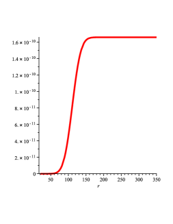
Figure 1: The function providing the gauge fixing, shown for $\sigma=0.05$, $G=10^{-11}$, $R_{S}=2$, $r_{0}=100$.

In terms of $f$ one can solve (24) for $P_{\Lambda}$. The closed form expression is again lengthy. Asymptotically for large $r$ we have $P_{\Lambda}=c_{0}r^{3/2}$ with $c_{0}$ a constant.

This completes the determination of the initial data. We need to fix the gauge for all time. To do this, we consider the preservation of $f(t,r)=X$, which determines the lapse. We would like the lapse, at least asymptotically, to reproduce the usual manifestly asymptotically flat nature of the Schwarzschild space-time. This corresponds to $N=1$ (recall that we are referring to $N_{\rm new}=1$, which corresponds asymptotically to $N_{\rm old}=1/\Lambda$). This results, asymptotically in $X=X_{\rm asymp.}+A(r)t$, where $X_{\rm asymp.}$ is the asymptotic value of the expression of $f$, which, for instance, can be read off for large values of $r$ in the figure above. The expression of $A(r)$ is,

$$A(r)=c_{1}r^{4}\exp\left(-\frac{1}{2}\left(r-r_{0}\right)^{2}\sigma^{2}\right),$$ (33)

with $c_{1}$ a constant.

With this form of the gauge fixing, the asymptotic form of the metric is,

$$g_{tt} = -1+\frac{2GM}{r},$$ (34)

$$g_{tr} = \frac{P_{\Lambda}}{\sqrt{r^{2}+P_{\Lambda}^{2}-2GMr}},$$ (35)

$$g_{rr} = \frac{r^{2}}{r^{2}+P_{\Lambda}^{2}-2GMr},$$ (36)

with $GM=R_{S}/2+X_{\rm asymp.}$, which shows that the asymptotic mass is the same as that of the horizon plus the contribution of the scalar field. With a simple redefinition of $t$ this yields the usual expression of the Schwarzschild metric in the Schwarzschild coordinates.

Although we have not studied the evolution in detail, one can envision using a gauge with (32) modified to be an ingoing pulse and this should yield real expressions for all quantities as the pulse travels inward, at least far away from the black hole.

V Discussion

We have shown that one can gauge fix spherically symmetric gravity coupled to a scalar field in terms of the traditional metric variables with a Hamiltonian that is the integral of a local density in explicit form. We construct a family of gauge fixings that can accommodate ingoing Gaussian pulses and show that they include manifestly asymptotically flat coordinates. The construction of the gauge is such that it is clear that it will evolve correctly in time, at least for a limited amount of time. It should be noted that we have not analyzed properly the inner boundary condition beyond the initial slice. One presumably would like to have a dynamical horizon that increases its mass as the ingoing pulses progress towards the black hole, at least studying the problem classically. Quantum mechanically, it is less clear what one needs at the horizon, since Hawking radiation should be present.

The question of quantization of the model in terms of this gauge implies having to deal with the quartic equation (24) that generically will lead to complex values. It is therefore unclear that the constructed Hamiltonian could be promoted to a self-adjoint operator. It should be noted that there exist techniques techniques to deal with these types of issues in quantization. We have recently illustrated this in a model system nosotrosmodelo . They are however, limited to certain regimes. Realistically, this type of approach is unlikely to yield insights about extreme regimes like the ones close to the singularity. But it may be useful in other situations, like in those in which a large black hole emits Hawking radiation to study, for instance, the back reaction of the weak radiation on the large black hole.

- (1) B. Berger, D. Chitre, Y. Nutku, V. Moncrief, Phys. Rev. D5, 2467 (1972).
- (2) W. Unruh, Phys. Rev. D14, 870 (1976).
- (3) V. Husain, O. Winkler, Phys. Rev. D71, 104001 (2005). [gr-qc/0503031]. R. G. Daghigh, G. Kunstatter, J. Gegenberg, Class. Quant. Grav. 24, 2099-2107 (2007).
- (4) W. Unruh, personal communication.
- (5) J. Gegenberg and G. Kunstatter, Phys. Rev. D 85, 084011 (2012) [arXiv:1112.3301 [gr-qc]]
- (6) K. V. Kuchar, Phys. Rev. D50, 3961-3981 (1994). [gr-qc/9403003].
- (7) K. Giesel and T. Thiemann, Class. Quant. Grav. 27, 175009 (2010) [arXiv:0711.0119 [gr-qc]]; R. Gambini, J. Pullin, in preparation.
- (8) R. Gambini, J. Pullin, “Self-adjointness in the Hamiltonians of deparameterized totally constrained theories: a model” [arXiv:1207.5730 [gr-qc]]