Phases and relativity in atomic gravimetry

Abstract

The phase observable measured by an atomic gravimeter built up on stimulated Raman transitions is discussed in a fully relativistic context. It is written in terms of laser phases which are invariant under relativistic gauge transformations. The dephasing $\Phi$ is the sum of light and atomic contributions which are connected to one another through their interplay with conservation laws at the interaction vertices. In the case of a closed geometry, a compact form of the dephasing is written in terms of a Legendre transform of the laser phases. These general expressions are illustrated by discussing two techniques used for compensating the Doppler shift, one corresponding to chirped frequencies and the other one to ramped variations.

I Introduction

After years of development, matter-wave interferometers have become accurate tools for measuring gravity fields. Matter-wave gravimeters were realized by using first neutron matter-waves Colella75 ; Staudenmann80 ; Klein83 ; Greenberger83 and then cold atoms matter-waves Kasevich91 ; Fixler07 ; Bouyer07 ; LeGouet0710 . These instruments are expected to open new roads to fundamental tests in relativistic, gravitational or quantum physics Dimopoulos07 ; Arvanitaki08 ; Ertmer09 ; Wolf09 ; Amelino09 ; Stockton11 . They have been studied in a number of detailed publications Borde89 ; Kasevich92 ; CohenTannoudji93 ; Storey94 ; Wolf99 ; Peters01 ; Borde02 ; Borde08 ; Dimopoulos08 ; Cronin09 .

Atomic interferometry experiments may be used to test the universality of free fall (UFF) by comparing the free fall of quantum bodies to that of classical test masses Peters99 . A recent claim Mueller10 has however blurred this up to then clear interpretation. The claim changes the interpretation of atom gravimetry experiments now considered as measuring the redshift on the quantum clock operating at a high Compton frequency. After this re-interpretation, these experiments would be considered as testing the universality of clock rates (UCR). The new interpretation has been contradicted WolfMueller10 and opened a debate on the significance of atom interferometry measurements in the context of relativity Sinha11 ; Giulini11 ; Unni11 ; Wolf11 ; HohenseeWolf12 ; Hohensee11 ; Wolf12 ; Schleich12 .

It is the aim of the present paper to present calculations of phase observables in a relativistic context and to stress points which are important for any study of this problem in metric theories. First, the phase observables involved in atomic interferometry are gauge invariant quantities. We will of course make references to coordinate systems but an important aim will be to write equations or statements independently of the specific choice of the coordinate system. Then, the expressions of the phase observables is intimately related to the conservation laws which constrain the description of interaction vertices. We will thus be careful to give a full account of conservation laws, and to make explicit their intimate connections with the expressions of phase observables.

The main focus of this paper is the effect of a uniform acceleration and we will in particular disregard the effect of gravity gradients, gravitational waves or rotations. This means that we study the unperturbed operation of atomic interferometers designed to measure the perturbation associated with a Riemann curvature Lamine02 ; Delva06 ; Dimopoulos08b ; Tino11 ; MIGA .

II Relativistic gravimetry

We consider an atomic gravimeter based on stimulated Raman interactions Kasevich92 which monitors the free fall of atoms with respect to an experimental platform at rest in the laboratory frame $\mathcal{R}$. We focus the attention on the case of a gravimeter measuring a stationary acceleration with no rotation and no curvature. This case may be represented by the Møller metric Moller52 ; Rohrlich63

$$\mathrm{d}s^{2}=\left(1+\gamma z\right)^{2}\left(c\mathrm{d}t\right)^{2}-\left(\mathrm{d}x^{2}+\mathrm{d}y^{2}+\mathrm{d}z^{2}\right)\,.$$ (1)

The metric element $\mathrm{d}s^{2}$ defines proper time Landau , with $\mathrm{d}s^{2}=c^{2}\mathrm{d}\tau^{2}$. The parameter $\gamma$ has the meaning of an acceleration divided by $c^{2}$.

As the Riemann curvature vanishes, the same physical situation may be described in a Minkowski frame $\overline{\mathcal{R}}$

$$\mathrm{d}s^{2}=\left(c\mathrm{d}\overline{t}\right)^{2}-\left(\mathrm{d}\overline{x}^{2}+\mathrm{d}\overline{y}^{2}+\mathrm{d}\overline{z}^{2}\right)\,.$$ (2)

The Møller map from (1) to (2) may be written under the reciprocal forms ($x,y$ unaffected)

$$1-\eta\gamma\overline{u}^{\eta}=\left(1+\gamma z\right)e^{-\eta\gamma ct}\;,$$ (3)

$$2\gamma ct=\ln\left(1+\gamma\overline{u}^{-}\right)-\ln\left(1-\gamma\overline{u}^{+}\right)\;,$$

$$1+\gamma z=\sqrt{\left(1-\gamma\overline{u}^{+}\right)\left(1+\gamma\overline{u}^{-}\right)}\;,$$

where we have introduced the two light cone variables

$$\overline{u}^{\eta}\equiv c\overline{t}-\eta\overline{z}\;,\quad\eta=\pm 1\,.$$ (4)

$\mathcal{R}$ is the laboratory frame in which the experimental platform is at rest while $\overline{\mathcal{R}}$ is the free fall frame in which atomic probes have inertial motions. They are convenient for different parts of the discussions.

The motions have a simple characterization in the Minkowskian frame $\overline{\mathcal{R}}$. They correspond to inertial motions with a uniform velocity $\eta c$ for light and $\overline{V}$ for matter with $\left|\overline{V}\right|\ll c$. They may be labeled by the set of associated conserved quantities, namely the energy $\overline{E}$, the momentum $\overline{P}$ and the boost generator

$$\overline{K}=\overline{E}\overline{z}-\overline{P}c^{2}\overline{t}=\overline{E}\overline{z_{0}}-\overline{P}c^{2}\overline{t_{0}}\,.$$ (5)

As $\overline{E},\overline{P},\overline{K}$ are conserved, eq.(5) gives the equation of motion in $\overline{\mathcal{R}}$ as well as in $\mathcal{R}$ (using (3))

$$\overline{E}+\gamma\overline{K}=\left(1+\gamma z\right)\left(\overline{E}\cosh(\gamma ct)-\overline{P}c\sinh(\gamma ct)\right)\,.$$ (6)

Equation (6) also expresses conservation of the energy $E$ defined in the stationary frame $\mathcal{R}$

$$E=\overline{E}\frac{\partial\overline{t}}{\partial t}-\overline{P}\frac{\partial\overline{z}}{\partial t}=\overline{E}+\gamma\overline{K}\,.$$ (7)

The last equations may be written similarly for the motions of light waves labeled by conserved quantities $\overline{e},\overline{p},\overline{k}$ (lowercase letters are used for light, uppercase letters for atoms). The equation of motion is written

$$\overline{k}=\overline{e}\overline{z}-\overline{p}c^{2}\overline{t}=-\eta\overline{e}\overline{u}^{\eta}$$ (8)

for light waves with velocity $\eta c$ and momentum $\overline{p}=\eta\overline{e}/c$ (assuming $x,y$ constant). It corresponds to a constant light cone variable $\overline{u}^{\eta}$ and may be written also in $\mathcal{R}$

$$e=\overline{e}+\gamma\overline{k}=\overline{e}\left(1+\gamma z\right)e^{-\eta\gamma ct}\,.$$ (9)

This fixes relations between the quantities $e$, $\overline{e}$, $\overline{k}$ and $\overline{u}^{\eta}$ which are conserved along each light motion

$$\overline{e}=\frac{e}{1-\eta\gamma\overline{u}^{\eta}}\quad,\quad\overline{k}=-\frac{\eta e\overline{u}^{\eta}}{1-\eta\gamma\overline{u}^{\eta}}\,.$$ (10)

This is also equivalent to the dependence of the Doppler effect on position in an accelerated frame Einstein07 ; Jaekel96 .

Matter and light waves are coupled through stimulated Raman interactions Kasevich92 at the vertices. Laser beams are delivered by sources at rest at position $z=z^{\mathrm{a}}$ in $\mathcal{R}$, which is translated into an accelerated motion in $\overline{\mathcal{R}}$ Rindler77

$$\left(1+\gamma z^{\mathrm{a}}\right)^{2} = \left(1-\gamma\overline{u}^{+}\right)\left(1+\gamma\overline{u}^{-}\right)$$ (11)

$$= \left(1-\gamma\overline{z}\right)^{2}-\left(\gamma c\overline{t}\right)^{2}\,.$$

The phases of these laser beams are discussed later on.

The geometry of the atomic gravimeter is sketched on the space-time diagram of Figure 1. This diagram is drawn in the free fall frame $\overline{\mathcal{R}}$ but it may be drawn as well in any other frame, say $\mathcal{R}$. Differences between the drawings are only apparent since they result from an arbitrary choice of the coordinate system. Intrinsic statements bear on gauge-invariant properties which do not depend on this choice. One aim of the present paper is to associate gauge invariant evaluations and statements to the geometrical drawing of Figure 1.

The conventions on Figure 1 have been chosen close to that of atomic physics calculations Storey94  : the space component $z$ is along the ordinate axis and the time component $ct$ along the abscissa; the units are chosen unequal in order to represent atomic velocities (much smaller than $c$); the proportions are altered so that light velocities are also apparent on the drawing. The representation could be brought back to the one commonly used in relativity (with $z$ along the abscissa and $ct$ along the ordinate axis; see for example Fig. 1 in Dimopoulos08 ) through a mirror reflection with respect to the bisecting line between the two coordinate axis.

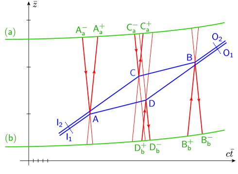
Figure 1: Space-time diagram for the atomic gravimeter in the free fall frame $\overline{\mathcal{R}}$. Blue, red and green lines represent the motions of atoms, light and laser sources respectively. Stimulated Raman interactions take place at the vertices $\mathsf{A}$, $\mathsf{B}$, $\mathsf{C}$, $\mathsf{D}$ where atomic and light lines intersect. Light phases are delivered at the intersections of light and laser lines (details in the text). The dotted lines $\mathsf{I}_{1}:\mathsf{I}_{2}$ and $\mathsf{O}_{1}:\mathsf{O}_{2}$ represent phase reference planes respectively at the input and output of the interferometer. The ticks on the axes show the units chosen for abscissa $c\overline{t}$ and ordinate $\overline{z}$. [Colors online]

The blue, red and green lines on Figure 1 represent the motions of atoms, light and lasers respectively (colors online). Two atomic (blue) paths are represented, and the interference between these two paths defines the dephasing (details below). On each path, inertial segments are joined by stimulated Raman vertices $\mathsf{A}$, $\mathsf{B}$, $\mathsf{C}$, $\mathsf{D}$ (letters chosen to match Fig. 9 in Storey94 ). The photon paths represent laser beams which have a propagation direction indicated by a $\pm$ sign and cross atomic lines at vertices $\mathsf{A}$, $\mathsf{B}$, $\mathsf{C}$, $\mathsf{D}$. The photon paths also intersect the laser lines $(\mathsf{a})$ and $(\mathsf{b})$ which sit respectively above and below the atoms. The intersection events are denoted by $\mathsf{A}^{\eta}_{\mathsf{a,b}}$, $\mathsf{B}^{\eta}_{\mathsf{a,b}}$, $\mathsf{C}^{\eta}_{\mathsf{a,b}}$ and $\mathsf{D}^{\eta}_{\mathsf{a,b}}$ on Figure 1. The drawing on Figure 1 is an idealized representation of the atomic gravimeter with the experimental setup simplified as much as possible while keeping the essential ingredients.

One of these essential ingredients is the link between phases and conservation laws. As the atoms are freely falling in the time intervals between interactions, they are accelerated with respect to experimental platforms at rest on ground. The Doppler shift induced by the free fall has thus to be compensated so that the stimulated Raman transitions are on resonance at the different vertices (see for example the footnote 49 in Dimopoulos08 ). Two techniques which have been used for this compensation Peters01 ; Cheinet06 will be discussed later on and considered as illustrations of the general expressions obtained in the present paper. There exists a small tolerance for the compensation of the Doppler shift, which is much more easily met under zero gravity conditions vanZoest10 ; Geiger11 . In the present paper, we restrict our attention to experiments performed in the typical Earth gravity $g\sim 9.81$m/s². Compensation of the Doppler shift induced by the free fall is thus mandatory, and we have to account carefully for the consequences of this compensation (details below).

In order to accommodate the various techniques used for that compensation, we will consider the laser phases as functions $\overline{\phi}^{\eta}\left(\overline{u}^{\eta}\right)$ of the light-cone variables $\overline{u}^{\eta}$. These laser phases are scalar quantities and may be written in any coordinate system

$$\overline{\phi}^{\eta}\left(\overline{u}^{\eta}\right)={\phi}^{\eta}\left(t,z\right)\,.$$ (12)

The derivatives of these functions are the photon energies which are involved in resonance conditions at vertices

$$\overline{e}^{\eta}\equiv\hbar c\overline{\kappa}^{\eta}\quad,\quad\overline{\kappa}^{\eta}\equiv\frac{\mathrm{d}\overline{\phi}^{\eta}}{\mathrm{d}\overline{u}^{\eta}}\quad,$$ (13)

$${e}^{\eta}\equiv\hbar c{\kappa}^{\eta}\quad,\quad{\kappa}^{\eta}\equiv\frac{\mathrm{d}{\phi}^{\eta}}{c\mathrm{d}t}\,.$$

The transformation between $\overline{e}^{\eta}$ and ${e}^{\eta}$ is given in (9).

The variation of the phase functions $\overline{\phi}^{\eta}$ fixes the energies and, then, the shape of the interferometer through the conservation laws. The same functions appear in the phase transfer from light to matter at the vertices of the interferometer. We will show in the next sections that these functions determine in fact all the terms involved in the expression of the dephasing.

III Phases and conservation laws

We now discuss phases for freely propagating atomic and light fields as well as at interaction vertices. These elementary building blocks will then be used to write the expression of the dephasing in the interferometer.

Spin properties are disregarded throughout this paper, for matter and light waves (see Borde89 ; Storey94 for discussions). Then, the internal energies (energies in the atomic rest frame) are fixed by atomic structure properties. They are the same on opposite atomic lines of the interferometer (see Fig. 9 in Storey94 ) with the mass difference $M_{\ast}-M$ between adjacent lines defined by the hyperfine structure ($\sim$9.2GHz for Caesium-133 atoms for instance). Its value is small with respect to laser frequencies but it is certainly not zero and has to be accounted for in relativistic calculations Borde08 .

With each atomic line drawn on Figure 1 is associated a Klein-Gordon field $\Psi(x)=F(x)e^{-i\Phi(x)}$ written as the product of a slowly varying envelop $F$ and of a rapidly varying phase $\Phi$. Similar relations hold for the light fields with lowercase letters $\psi$, $f$, $\phi$ and $p_{\mu}$ replacing $\Psi$, $F$, $\Phi$ and $P_{\mu}$. With each vertex $\mathsf{A}$, $\mathsf{B}$, $\mathsf{C}$, $\mathsf{D}$ on Figure 1 is associated an equation relating the fields involved in the stimulated Raman interaction. In a simplified approach, the outgoing matter fields are given by incoming matter fields and light fields (more general solutions discussed for example in Borde02 )

$$\Psi_{\mathsf{A}}^{\mathrm{out}}=\Psi_{\mathsf{A}}^{\mathrm{in}}\psi_{\mathsf{A}}^{-}\left(\psi_{\mathsf{A}}^{+}\right)^{\ast}\,,\,\Psi_{\mathsf{C}}^{\mathrm{out}}=\Psi_{\mathsf{C}}^{\mathrm{in}}\psi_{\mathsf{C}}^{-}\left(\psi_{\mathsf{C}}^{+}\right)^{\ast}\,,$$

$$\Psi_{\mathsf{B}}^{\mathrm{out}}=\Psi_{\mathsf{B}}^{\mathrm{in}}\psi_{\mathsf{B}}^{+}\left(\psi_{\mathsf{B}}^{-}\right)^{\ast}\,,\,\Psi_{\mathsf{D}}^{\mathrm{out}}=\Psi_{\mathsf{D}}^{\mathrm{in}}\psi_{\mathsf{D}}^{+}\left(\psi_{\mathsf{D}}^{-}\right)^{\ast}\,.$$ (14)

The labels “in” and “out” correspond to incoming and outgoing matter waves defined in the close vicinity of the vertex while “-” and “+” correspond to light waves propagating respectively downward and upward. The light fields $\psi$ and $\psi^{\ast}$ correspond to positive and negative frequency parts of the waves and they are associated respectively with absorption and stimulated emission processes. Equations are the same at $\mathsf{A}$ and $\mathsf{C}$ where the atom absorbs a downward photon and emits an upward one, and changed through the exchange of +/- sign at vertices $\mathsf{B}$ and $\mathsf{D}$ where the atom absorbs an upward photon and emits a downward one. This difference is indicated on the geometrical drawing of Figure 1 by thick red lines which bear the absorbed and emitted photons and arrows which indicate the propagation directions. The multiplicative relations (14) for the waves are translated into additive ones for the phases

$$\Phi_{\mathsf{A}}^{\mathrm{out}}=\Phi_{\mathsf{A}}^{\mathrm{in}}+\phi_{\mathsf{A}}^{-}-\phi_{\mathsf{A}}^{+} \Phi_{\mathsf{C}}^{\mathrm{out}}=\Phi_{\mathsf{C}}^{\mathrm{in}}+\phi_{\mathsf{C}}^{-}-\phi_{\mathsf{C}}^{+}\,,$$ ,

$$\Phi_{\mathsf{B}}^{\mathrm{out}}=\Phi_{\mathsf{B}}^{\mathrm{in}}+\phi_{\mathsf{B}}^{+}-\phi_{\mathsf{B}}^{-} \Phi_{\mathsf{D}}^{\mathrm{out}}=\Phi_{\mathsf{D}}^{\mathrm{in}}+\phi_{\mathsf{D}}^{+}-\phi_{\mathsf{D}}^{-}\,.$$ , (15)

As energy and momentum are gradients of phases, the last equations lead through differentiation to energy-momentum conservation laws for the Raman interaction processes. We introduce lightcone notations for energy-momentum variables in $\overline{\mathcal{R}}$

$$\overline{P}^{\eta}\equiv\frac{1}{2}\left(\frac{\overline{E}}{c}+\eta\overline{P}\right)$$ (16)

in order to write the conservation laws

$$\overline{P}_{\mathsf{A}}^{\eta,\mathrm{out}}=\overline{P}_{\mathsf{A}}^{\eta,\mathrm{in}}-\frac{\eta\overline{e}_{\mathsf{A}}^{\eta}}{c}\,,\,\overline{P}_{\mathsf{C}}^{\eta,\mathrm{out}}=\overline{P}_{\mathsf{C}}^{\eta,\mathrm{in}}-\frac{\eta\overline{e}_{\mathsf{C}}^{\eta}}{c}\,,$$

$$\overline{P}_{\mathsf{B}}^{\eta,\mathrm{out}}=\overline{P}_{\mathsf{B}}^{\eta,\mathrm{in}}+\frac{\eta\overline{e}_{\mathsf{B}}^{\eta}}{c}\,,\,\overline{P}_{\mathsf{D}}^{\eta,\mathrm{out}}=\overline{P}_{\mathsf{D}}^{\eta,\mathrm{in}}+\frac{\eta\overline{e}_{\mathsf{D}}^{\eta}}{c}\,.$$ (17)

As the energies of the absorbed and emitted photons are close to each other, the effective energy transfer is small while the momentum transfer is significant, so that the main effect for the atom is to undergo a kick due to momentum conservation.

As the atomic momenta are conserved on the inertial motions between interactions, we can use the following relations to simplify (17)

$$\overline{P}_{\mathsf{A}}^{\eta,\mathrm{out}}=\overline{P}_{\mathsf{D}}^{\eta,\mathrm{in}}\equiv\overline{P}_{\mathsf{AD}}^{\eta} \overline{P}_{\mathsf{C}}^{\eta,\mathrm{out}}=\overline{P}_{\mathsf{B}}^{\eta,\mathrm{in}}\equiv\overline{P}_{\mathsf{CB}}^{\eta}\,.$$ , (18)

We also assume that the interferometer is adjusted for plane waves at its input and output ports. This means that momenta are identical in the two incoming legs of the interfering paths as well as in the outgoing legs

$$\overline{P}_{\mathsf{A}}^{\eta,\mathrm{in}}=\overline{P}_{\mathsf{C}}^{\eta,\mathrm{in}}\equiv\overline{P}_{\mathsf{I}}^{\eta} \overline{P}_{\mathsf{D}}^{\eta,\mathrm{out}}=\overline{P}_{\mathsf{B}}^{\eta,\mathrm{out}}\equiv\overline{P}_{\mathsf{O}}^{\eta}\,.$$ , (19)

Using these relations, we rewrite the conservation laws

$$\overline{P}_{\mathsf{AD}}^{\eta}=\overline{P}_{\mathsf{I}}^{\eta}-\frac{\eta\overline{e}_{\mathsf{A}}^{\eta}}{c}=\overline{P}_{\mathsf{O}}^{\eta}-\frac{\eta\overline{e}_{\mathsf{D}}^{\eta}}{c}\,,$$

$$\overline{P}_{\mathsf{CB}}^{\eta}=\overline{P}_{\mathsf{I}}^{\eta}-\frac{\eta\overline{e}_{\mathsf{C}}^{\eta}}{c}=\overline{P}_{\mathsf{O}}^{\eta}-\frac{\eta\overline{e}_{\mathsf{B}}^{\eta}}{c}\,,$$ (20)

and deduce

$$\overline{e}_{\mathsf{A}}^{\eta}+\overline{e}_{\mathsf{B}}^{\eta} = \overline{e}_{\mathsf{C}}^{\eta}+\overline{e}_{\mathsf{D}}^{\eta}$$

$$= \eta c\left(\overline{P}_{\mathsf{I}}^{\eta}+\overline{P}_{\mathsf{O}}^{\eta}-\overline{P}_{\mathsf{AD}}^{\eta}-\overline{P}_{\mathsf{CB}}^{\eta}\right)\,.$$

In order to account for all kinematical constraints, we also write the equality of masses $M^{2}\equiv\overline{P}^{+}\overline{P}^{-}/4c^{2}$ on opposite atomic lines of the interferometer

$${M}_{\mathsf{I}}^{2}={M}_{\mathsf{O}}^{2}\equiv M^{2} {M}_{\mathsf{AD}}^{2}={M}_{\mathsf{CB}}^{2}\equiv{M}_{\ast}^{2}\,.$$ , (22)

The associated constraints are conveniently written by introducing notations for the average values and differences of momenta on opposite sides

$$\overline{P}_{\mathsf{O}}^{\eta}\equiv\overline{P}^{\eta}+\frac{\Delta\overline{P}^{\eta}}{2} \overline{P}_{\mathsf{I}}^{\eta}\equiv\overline{P}^{\eta}-\frac{\Delta\overline{P}^{\eta}}{2}\,,$$ , (23)

$$\overline{P}_{\mathsf{AD}}^{\eta}\equiv\overline{P}_{\ast}^{\eta}+\frac{\Delta\overline{P}_{\ast}^{\eta}}{2} \overline{P}_{\mathsf{CB}}^{\eta}\equiv\overline{P}_{\ast}^{\eta}-\frac{\Delta\overline{P}_{\ast}^{\eta}}{2}\,,$$ ,

and deducing from (22)

$${\overline{e}_{\mathsf{D}}^{\eta}-\overline{e}_{\mathsf{A}}^{\eta}}={\overline{e}_{\mathsf{B}}^{\eta}-\overline{e}_{\mathsf{C}}^{\eta}}=\frac{\overline{E}+\eta c\overline{P}}{2\overline{E}}{c\Delta\overline{P}}\equiv{2\overline{\epsilon}^{\eta}}\,,$$ (24)

$${\overline{e}_{\mathsf{C}}^{\eta}-\overline{e}_{\mathsf{A}}^{\eta}}={\overline{e}_{\mathsf{B}}^{\eta}-\overline{e}_{\mathsf{D}}^{\eta}}=\frac{\overline{E}_{\ast}+\eta c\overline{P}_{\ast}}{2\overline{E}_{\ast}}c\Delta\overline{P}_{\ast}\equiv{2\overline{\epsilon}_{\ast}^{\eta}}\,.$$

It follows that all photon energies can be expressed from the four atomic momenta

$$\overline{e}_{\mathsf{A}}^{\eta}=\overline{e}^{\eta}-\overline{\epsilon}^{\eta}-\overline{\epsilon}_{\ast}^{\eta}\;,\;\overline{e}_{\mathsf{B}}^{\eta}=\overline{e}^{\eta}+\overline{\epsilon}^{\eta}+\overline{\epsilon}_{\ast}^{\eta}\;,$$

$$\overline{e}_{\mathsf{C}}^{\eta}=\overline{e}^{\eta}-\overline{\epsilon}^{\eta}+\overline{\epsilon}_{\ast}^{\eta}\;,\;\overline{e}_{\mathsf{D}}^{\eta}=\overline{e}^{\eta}+\overline{\epsilon}^{\eta}-\overline{\epsilon}_{\ast}^{\eta}\;,$$ (25)

where $\overline{e}^{\eta}$ denotes the mean photon energy (see eqs.III)

$$\overline{e}^{\eta}\equiv\frac{\overline{e}_{\mathsf{A}}^{\eta}+\overline{e}_{\mathsf{B}}^{\eta}}{2}=\frac{\overline{e}_{\mathsf{C}}^{\eta}+\overline{e}_{\mathsf{D}}^{\eta}}{2}=\eta c\left(\overline{P}^{\eta}-\overline{P}_{\ast}^{\eta}\right)\,.$$ (26)

As discussed in the previous section, the Doppler shift induced by the free fall of the atoms must be compensated so that the stimulated Raman transitions remain at resonance at the different vertices. Equations (25-26) provide the relations to be fulfilled by the laser frequencies so that this aim is met.

IV Dephasing of the interferometer

We now write the evolution of phases for free matter motions. We then combine the obtained expressions with those of the previous section to deduce the dephasing measured at the output of the interferometer.

For matter waves, the phase on an inertial motion, say the segment $\mathsf{AD}$ on Figure 1, may be written under any of the equivalent forms ($\Phi_{\mathsf{AD}}\equiv\Phi_{\mathsf{D}}^{\mathrm{in}}-\Phi_{\mathsf{A}}^{\mathrm{out}}$, $\tau_{\mathsf{AD}}\equiv\tau_{\mathsf{D}}^{\mathrm{in}}-\tau_{\mathsf{A}}^{\mathrm{out}}$ and $\overline{u}_{\mathsf{AD}}^{\eta}\equiv\overline{u}_{\mathsf{D}}^{\eta}-\overline{u}_{\mathsf{A}}^{\eta}$)

$$\hbar\Phi_{\mathsf{AD}}={M_{\mathsf{AD}}c^{2}\,\tau_{\mathsf{AD}}}={2\overline{P}_{\mathsf{AD}}^{+}\overline{u}_{\mathsf{AD}}^{+}}={2\overline{P}_{\mathsf{AD}}^{-}\overline{u}_{\mathsf{AD}}^{-}}\,.$$ (27)

The equivalence of these forms follows from the geometric identities valid on any inertial motion

$$\frac{2\overline{P}^{+}}{Mc}=\frac{Mc}{2\overline{P}^{-}}=\sqrt{\frac{\overline{P}^{+}}{\overline{P}^{-}}}=\sqrt{\frac{\mathrm{d}\overline{u}^{-}}{\mathrm{d}\overline{u}^{+}}}=\frac{c\mathrm{d}\tau}{\mathrm{d}\overline{u}^{+}}=\frac{\mathrm{d}\overline{u}^{-}}{c\mathrm{d}\tau}\,.$$ (28)

Note also that the identity of the two last expressions in (27) can be considered as a consequence of the conservation of boost generator (5) along an inertial motion

$$\overline{K}=\overline{P}^{-}\overline{u}^{-}-\overline{P}^{+}\overline{u}^{+}\quad,\quad\mathrm{d}\overline{K}=0\,.$$ (29)

Under its differential form, (27) means that $\hbar\mathrm{d}\Phi$ may be written as proportional to elapsed proper time $\mathrm{d}\tau$ or lightcone variables increments $\mathrm{d}\overline{u}^{\eta}$

$$\hbar\mathrm{d}\Phi=Mc^{2}\,\mathrm{d}\tau=2\overline{P}^{+}\mathrm{d}\overline{u}^{+}=2\overline{P}^{-}\mathrm{d}\overline{u}^{-}\,.$$ (30)

The first relation connects the methods of quantum theory, where classical trajectories extremize the action integrals, with metric theories, where geodesics extremize the proper time intervals Landau . The other relations imply that the matter phases are functionals of the conserved quantities which characterize the light rays involved at the interaction vertices. Note that for light waves, the phase is constant ($\mathrm{d}\phi=0$) or equivalently the proper time is freezed ($\mathrm{d}\tau=0$) along propagation. This is the basic idea of Einstein synchronization and localization which allow remote observers to exchange information by sharing the common value of a light phase Jaekel96 . Here we see that the same light phases are transcribed to atomic phases at the interaction vertices and become an essential part of the dephasing measured by the interferometer.

As the interferometer is adjusted for coherent matter waves at its input and output ports, the dephasing $\Phi$ is just the difference of phases accumulated on the two arms 1 and 2 (see Figure 1)

$$\Phi=\left(\Phi_{\mathsf{O}_{2}}-\Phi_{\mathsf{I}_{2}}\right)-\left(\Phi_{\mathsf{O}_{1}}-\Phi_{\mathsf{I}_{1}}\right)\,.$$ (31)

We collect the elementary relations written up to now, and deduce the dephasing (31) as follows

$$\Phi = \Phi_{\mathrm{li}}+\Phi_{\mathrm{at}}\quad,$$ (32)

$$\Phi_{\mathrm{li}} = \Phi_{\mathrm{li}}^{+}-\Phi_{\mathrm{li}}^{-}\quad,\quad\Phi_{\mathrm{li}}^{\eta}=\phi_{\mathsf{A}}^{\eta}+\phi_{\mathsf{B}}^{\eta}-\phi_{\mathsf{C}}^{\eta}-\phi_{\mathsf{D}}^{\eta}\quad,$$

$$\Phi_{\mathrm{at}} = \left(\Phi_{\mathsf{I}_{2}\mathsf{C}}+\Phi_{\mathsf{CB}}+\Phi_{\mathsf{B}\mathsf{O}_{2}}\right)-\left(\Phi_{\mathsf{I}_{1}\mathsf{A}}+\Phi_{\mathsf{AD}}+\Phi_{\mathsf{D}\mathsf{O}_{1}}\right)\,.$$

$\Phi_{\mathrm{li}}$ is the sum of phases transferred from light to atoms at the interaction vertices (see eqs.15) while $\Phi_{\mathrm{at}}$ is the sum of propagation phases (27) over atomic lines. Note that equation (32) is independent on the choice of the input and output reference planes $\mathsf{I}$ and $\mathsf{O}$ as well as on the choice of points $\mathsf{I}_{1}$ and $\mathsf{I}_{2}$ in the plane $\mathsf{I}$ or, equivalently, of points $\mathsf{O}_{1}$ and $\mathsf{O}_{2}$ in the plane $\mathsf{O}$. This is important since plane waves consist in coherent superpositions of all points on these phase planes. It is also worth stressing here that all terms appearing in (32) have a definition independent of the specific coordinate system used in the calculation. This means that they are gauge invariant in the general relativistic sense. One may remark that the sum $\Phi$ of light and atomic terms is also invariant under changes of electromagnetic gauge while being the physical observable measured in the interferometer.

The expression of $\Phi_{\mathrm{at}}$ in (32) contains the separation terms coming from the fact that the interferometer has not necessarily a closed geometry Borde08 ; Dimopoulos08 . A convenient convention is to have these reference planes just before the first vertex and just after the last vertex so that $\mathsf{I}_{1}\equiv\mathsf{A}\equiv\mathsf{A}_{1}$ and $\mathsf{O}_{2}\equiv\mathsf{B}\equiv\mathsf{B}_{2}$. Denoting respectively $\mathsf{A}_{2}$ and $\mathsf{B}_{1}$ the points on trajectories 2 and 1 which lie on the same reference planes as $\mathsf{A}$ and $\mathsf{B}$, one deduces

$$\Phi_{\mathrm{at}} = \left(\Phi_{\mathsf{A}_{2}\mathsf{C}}+\Phi_{\mathsf{C}\mathsf{B}_{2}}\right)-\left(\Phi_{\mathsf{A}_{1}\mathsf{D}}+\Phi_{\mathsf{D}\mathsf{B}_{1}}\right)\,.$$ (33)

Using the conservation laws (20), we deduce that $\Phi_{\mathrm{at}}$ may be written under either of the equivalent forms

$$\Phi_{\mathrm{at}} = \Phi_{\mathrm{at}}^{+}=-\Phi_{\mathrm{at}}^{-}=\frac{\Phi_{\mathrm{at}}^{+}-\Phi_{\mathrm{at}}^{-}}{2}\,,$$ (34)

where

$$\Phi_{\mathrm{at}}^{\eta}=-2\left(\overline{\kappa}_{\mathsf{A}}^{\eta}\overline{u}_{\mathsf{A}}^{\eta}+\overline{\kappa}_{\mathsf{B}}^{\eta}\overline{u}_{\mathsf{B}}^{\eta}-\overline{\kappa}_{\mathsf{C}}^{\eta}\overline{u}_{\mathsf{C}}^{\eta}-\overline{\kappa}_{\mathsf{D}}^{\eta}\overline{u}_{\mathsf{D}}^{\eta}\right)+\Phi_{\mathrm{sep}}^{\eta}\,,$$

$$\Phi_{\mathrm{sep}}^{\eta}=2\eta\frac{\overline{P}^{\eta}_{\mathsf{O}}\left(\overline{u}^{\eta}_{\mathsf{B}_{2}}-\overline{u}^{\eta}_{\mathsf{B}_{1}}\right)-\overline{P}^{\eta}_{\mathsf{I}}\left(\overline{u}^{\eta}_{\mathsf{A}_{2}}-\overline{u}^{\eta}_{\mathsf{A}_{1}}\right)}{\hbar}\,.$$ (35)

In (35), the separation terms $\Phi_{\mathrm{sep}}^{\eta}$ are written in terms of the input and output atomic momenta whereas the other terms in the first line depend only on the momenta transferred at vertices.

In order to make the discussion more explicit, let us now consider the case of a closed geometry with the interferometer adjusted so that $\mathsf{B}_{1}$ and $\mathsf{B}_{2}$ coincide when $\mathsf{A}_{1}$ and $\mathsf{A}_{2}$ coincide. After this adjustment, the separation terms $\Phi_{\mathrm{sep}}^{\eta}$ vanish and the dephasing is given by a compact expression collecting all contributions

$$\Phi = \Phi^{+}-\Phi^{-}\quad,$$ (36)

$$\Phi^{\eta} = \varphi_{\mathsf{A}}^{\eta}+\varphi_{\mathsf{B}}^{\eta}-\varphi_{\mathsf{C}}^{\eta}-\varphi_{\mathsf{D}}^{\eta}\quad,$$

$$\varphi^{\eta} \equiv \phi^{\eta}-\overline{\kappa}^{\eta}\overline{u}^{\eta}=\phi^{\eta}-\overline{u}^{\eta}\frac{\mathrm{d}{\phi}^{\eta}}{\mathrm{d}\overline{u}^{\eta}}\,.$$

Note that $\varphi^{\eta}$ is the Legendre transform of the laser phase $\phi^{\eta}$ and is more naturally considered as a function of the laser wavevector $\overline{\kappa}^{\eta}$ with the relations $\mathrm{d}{\phi}^{\eta}=\overline{\kappa}^{\eta}\mathrm{d}\overline{u}^{\eta}$ and $\mathrm{d}{\varphi}^{\eta}=-\overline{u}^{\eta}\mathrm{d}\overline{\kappa}^{\eta}$.

The forthcoming discussions will be presented in this case of a closed geometry where the dephasing is given by the expression (36), completely characterized by the Legendre transform of the laser phases at the 4 events $\mathsf{A}$, $\mathsf{B}$, $\mathsf{C}$ and $\mathsf{D}$. Note that, if needed, one may come back to the general case by adding the separation terms written in (35).

V Discussion

We now illustrate the expression (36) obtained in the preceding section for a closed interferometer by discussing two techniques which have been used for compensating the Doppler shift. One such technique corresponds to chirped frequencies with the chirp parameter being adjusted Cheinet06 . Another one, described by Figure. 13 in Peters01 , corresponds to ramped variations, with Raman laser frequencies constant by pieces and changed between vertices.

We first consider the case where the laser frequencies are chirped so that resonance is preserved with freely falling atoms Cheinet06 . This can be described within the following family of parameterizations of light phases

$$\phi^{\eta}=\phi_{0}^{\eta}-\frac{\omega^{\eta}}{c}\left(\frac{1-\alpha}{\eta\gamma}\ln\left(1-\eta\gamma\overline{u}^{\eta}\right)-\alpha\overline{u}^{\eta}\right)\,.$$ (37)

The variations of associated energies are deduced from (13) (with $\omega^{\eta}$, $\alpha$ and $\phi_{0}^{\eta}$ constant)

$$\overline{e}^{\eta}=\hbar c\overline{\kappa}^{\eta}=\hbar\omega^{\eta}\frac{1-\eta\alpha\gamma\overline{u}^{\eta}}{1-\eta\gamma\overline{u}^{\eta}}\quad,$$

$${e}^{\eta}=\hbar c\kappa^{\eta}=\hbar\omega^{\eta}\left(1-\eta\alpha\gamma\overline{u}^{\eta}\right)\,.$$ (38)

With the chirp parameter $\alpha$ set to 0, ${\kappa}^{\eta}$ is constant and the interferometer cannot operate properly because of the Doppler shift induced by free fall. With $\alpha$ set to 1 in contrast, $\overline{\kappa}^{\eta}$ is constant, and the resonance conditions are met at the 4 vertices in a symmetric geometry where the interferometer has the shape of a parallelogram. Atomic momenta are equal on opposite sides, so that atoms spend equal proper times on opposite sides. It follows that the atomic part of the dephasing is obviously zero ($\Phi_{\mathrm{at}}=0$) as a consequence of this symmetry.

This symmetry also entails that the light part of the dephasing vanishes, though in a more indirect manner. As a matter of fact, the momenta $\overline{\kappa}^{\eta}$ are equal at the 4 vertices (for each value of $\eta$ taken separately), so that the derivatives of the phase functions $\phi^{\eta}$ are equal at $\mathsf{A}$, $\mathsf{B}$, $\mathsf{C}$ and $\mathsf{D}$. Within the family of parameterizations (37), the derivatives $\overline{\kappa}^{\eta}$ are thus constant everywhere (not only at the vertices), and phases $\phi^{\eta}$ are linear functions of the lightcone variables $\overline{u}^{\eta}$. Then the light part $\Phi_{\mathrm{li}}$ of the dephasing also vanishes because of the symmetry of the interferometer. This remark has been used as the starting point for a measurement procedure for the acceleration. This is the procedure explained in Cheinet06  : when the chirp parameter $\alpha\gamma$ appearing in the law of variation (38) of $\kappa^{\eta}$ is varied in parameterizations (37), both contributions $\Phi_{\mathrm{at}}$ and $\Phi_{\mathrm{li}}$ to the dephasing $\Phi$ vanish simultaneously at $\alpha=1$. The specific value of this chirp parameter producing a null dephasing thus leads to a determination of the value of the acceleration parameter $\gamma$.

Equation (36) can be used for a fast demonstration of the fact that the full dephasing vanishes in this case. As a matter of fact, when $\alpha=1$ in (37), the Legendre transform $\varphi^{\eta}$ of the phase is constant, so that the combination $\varphi_{\mathsf{A}}^{\eta}+\varphi_{\mathsf{B}}^{\eta}-\varphi_{\mathsf{C}}^{\eta}-\varphi_{\mathsf{D}}^{\eta}$ appearing in (36) is obviously zero. This fast line is also useful for evaluating the dominant terms in the vicinity of $\alpha=1$ (development in the small parameter $\alpha-1$)

$$\frac{c\Phi^{\eta}}{\omega^{\eta}} = \left(\alpha-1\right)\frac{\eta\gamma}{2}\left(\overline{u}^{\eta\ 2}_{\mathsf{A}}+\overline{u}^{\eta\ 2}_{\mathsf{B}}-\overline{u}^{\eta\ 2}_{\mathsf{C}}-\overline{u}^{\eta\ 2}_{\mathsf{D}}\right)$$

$$+ \left(\alpha-1\right)\frac{2\gamma^{2}}{3}\left(\overline{u}^{\eta\ 3}_{\mathsf{A}}+\overline{u}^{\eta\ 3}_{\mathsf{B}}-\overline{u}^{\eta\ 3}_{\mathsf{C}}-\overline{u}^{\eta\ 3}_{\mathsf{D}}\right)+\ldots$$

As the higher order terms decrease rapidly since $\gamma\overline{u}$ are small dimensionless numbers, this expression is dominated by the second order term. In perturbation theory, one may then calculate this term in the symmetric configuration which corresponds to $\alpha=1$. In order to do so, we introduce the middle point $\mathsf{M}$ of the parallelogram and use the following relations

$$\overline{u}^{\eta}_{\mathsf{B}}-\overline{u}^{\eta}_{\mathsf{M}}=\overline{u}^{\eta}_{\mathsf{M}}-\overline{u}^{\eta}_{\mathsf{A}}=\frac{\overline{u}^{\eta}_{\mathsf{B}}-\overline{u}^{\eta}_{\mathsf{A}}}{2}\,,$$

$$\overline{u}^{\eta}_{\mathsf{D}}-\overline{u}^{\eta}_{\mathsf{M}}=\overline{u}^{\eta}_{\mathsf{M}}-\overline{u}^{\eta}_{\mathsf{C}}=\frac{\overline{u}^{\eta}_{\mathsf{D}}-\overline{u}^{\eta}_{\mathsf{C}}}{2}\,.$$ (40)

We then obtain an expression of the dephasing in terms of the diagonals of the parallelogram

$$\frac{c\Phi^{\eta}}{\omega^{\eta}}\simeq\left(\alpha-1\right)\frac{\eta\gamma}{4}\left((\overline{u}^{\eta}_{\mathsf{B}}-\overline{u}^{\eta}_{\mathsf{A}})^{2}-(\overline{u}^{\eta}_{\mathsf{D}}-\overline{u}^{\eta}_{\mathsf{C}})^{2}\right)\,.$$ (41)

If one also uses the approximations that the atoms have non relativistic velocities and that the momenta transferred at vertices are small, one finally obtains

$$\Phi \sim k_{\mathrm{eff}}\left(\alpha-1\right)\gamma c^{2}T^{2}\quad,\quad k_{\mathrm{eff}}=\frac{\omega^{+}+\omega^{-}}{c}\,.$$ (42)

As is well-known, the dephasing is thus determined by the laser wavevectors entering the definition of $k_{\mathrm{eff}}$ (and not by the Compton wavelength associated with the mass of the atoms).

We now discuss another measurement procedure, which corresponds to the ramped phase functions sketched on Fig. 13 in Peters01 . In this case, $\kappa$ is supposed to be constant during intervals of time and to undergo jumps between the vertices so that resonance conditions are still met (at least approximately) at the 4 vertices. The phase functions thus correspond to (37) with $\alpha=0$ on three intervals $i=1,2,3$ containing $\mathsf{A}$ for the first, $\mathsf{C}$ and $\mathsf{D}$ for the second, $\mathsf{B}$ for the third

$$\phi^{\eta}=\phi_{i}^{\eta}-\frac{\omega^{\eta}_{i}}{\eta\gamma c}\ln\left(1-\eta\gamma\overline{u}^{\eta}\right)\,.$$ (43)

Accordingly, the energies correspond to (38) with $\alpha=0$

$$\overline{e}^{\eta}=\hbar c\overline{\kappa}^{\eta}=\frac{\hbar\omega^{\eta}_{i}}{1-\eta\gamma\overline{u}^{\eta}}\quad,\quad{e}^{\eta}=\hbar c{\kappa}^{\eta}=\hbar\omega^{\eta}_{i}\,.$$ (44)

The energies are discontinuous at the jumps while the phases are continuous Peters01 .

The parameters are then adjusted so that phases and energies at the vertices are as close as possible to those obtained in the chirped case. This can be done exactly at $\mathsf{A}$, $\mathsf{B}$, and $\mathsf{M}$ but not at the two points $\mathsf{C}$ and $\mathsf{D}$. There remain small defects because this compensation technique cannot meet the resonance prescription at the two points $\mathsf{C}$ and $\mathsf{D}$. One deduces in particular from (44) that

$$\frac{\overline{\kappa}^{\eta}_{\mathsf{D}}}{\overline{\kappa}^{\eta}_{\mathsf{C}}}=\frac{1-\eta\gamma\overline{u}^{\eta}_{\mathsf{C}}}{1-\eta\gamma\overline{u}^{\eta}_{\mathsf{D}}}\,.$$ (45)

Meanwhile, this ratio should be 1 for the compensation to be exact, which corresponds to the fact that the phases (43) do not reproduce exactly the law (37) with $\alpha=1$ which led to a null dephasing. The order of magnitude of these defects is however small as the two points $\mathsf{C}$ and $\mathsf{D}$ are close to each other in the conditions of the experiments Peters01 . This entails that this second method leads to results close to that of the first one.

VI Conclusion

In the present paper, we have emphasized the status of relativistic observable of the phase measured by an atomic gravimeter. In particular, we have written it in terms of laser phases which are invariant under relativistic gauge transformations (they do not depend on the choice of the coordinate system). The physical observable $\Phi$, which is the sum of light and atomic contributions to the dephasing, is also invariant under electromagnetic gauge transformations.

We have also studied in a detailed manner the interplay of the expressions thus obtained with conservation laws at the interaction vertices. The general expression of the dephasing is given by equations (32) and (35) for an arbitrary geometry and by the more compact form (36) when the interferometer is adjusted to have a closed geometry. This compact form, which is given by a Legendre transform of the laser phases, makes obvious the intimate connection between light and atomic contributions to the dephasing.

We have finally illustrated these general expressions by discussing two techniques which have been used for compensating the Doppler shift, one corresponding to chirped frequencies and the other one to ramped variations. We have thus recovered the known result that the dephasing is determined by the momenta transferred at the vertices, i.e. by the laser wavevectors (and not by the Compton wavelength associated with the mass of the atoms).

- (1) Colella R., Overhauser A. W. and Werner S. A., Phys. Rev. Lett. 34 1472 (1975)
- (2) Staudenmann J.-L., Werner S. A., Colella R. and Overhauser A. W., Phys. Rev. A 21 1419 (1980)
- (3) Klein A. G. and Werner S. A., Rep. Prog. Phys. 46 259 (1983)
- (4) Greenberger D. M., Rev. Mod. Phys. 55 875 (1983)
- (5) Kasevich M. A., and Chu S., Phys. Rev. Lett. 67 181 (1991)
- (6) Fixler J. B., Foster G. T., McGuirk J. M., Kasevich M. A., Science 315 74 (2007)
- (7) Bouyer P., Pereira Dos Santos F., Landragin A. and Bordé C. J., in Lasers, Clocks, and Drag Free: Exploration of Relativistic Gravity in Space eds H. Dittus et al (Springer, 2007) 297
- (8) Le Gouët J., Cheinet P., Kim J. et al, Eur. Phys. J. D 44 419 (2007); Le Gouët J., Merlet S., Bodard Q., Malossi N., et al, Metrologia 47 L9 (2010)
- (9) Dimopoulos S., Graham P. W., Hogan J. M., and Kasevich M. A., Phys. Rev. Lett. 98 111102 (2007)
- (10) Arvanitaki A., Dimopoulos S., Geraci A. A. et al. Phys. Rev. Lett. 100 120407 (2008)
- (11) Ertmer W., Schubert C., Wendrich T., et al, Exp. Astronomy 23 611 (2009)
- (12) Wolf P., Bordé C. J., Clairon A., et al, Exp. Astronomy 23 651 (2009)
- (13) Amelino-Camelia G., Aplin K., Arndt M., et al, Exp. Astronomy 23 549 (2009)
- (14) Stockton J. K., Takase K., Kasevich M. A. Phys. Rev. Lett. 107 133001 (2011)
- (15) Bordé C.J., Phys. Lett. 140 10 (1989)
- (16) Kasevich M. A., and Chu S., App. Phys. B 54 321 (1992)
- (17) Cohen-Tannoudji C., Cours au Collège de France (1992-93) [http://www.phys.ens.fr/cours/college-de-france/1992-93/1992-93.htm] (in french)
- (18) Storey P., and Cohen-Tannoudji C., J. Physique II 4 1999 (1994)
- (19) Wolf P., and Tourrenc P., Phys. Lett. A 251 241 (1999)
- (20) Peters A., Chung K.Y. and Chu S., Metrologia 38 25 (2001)
- (21) Bordé C.J., Metrologia 39 435 (2002)
- (22) Bordé C.J., Eur. Phys. J. Spec. Top. 163 315 (2008)
- (23) Dimopoulos S., Graham P. W., Hogan J. M., and Kasevich M. A., Phys. Rev. D 78 042003 (2008)
- (24) Cronin A. D., Schmiedmayer J., and Pritchard D. E., Rev. Mod. Phys. 81 1051 (2009)
- (25) Peters A., Chung K.Y. and Chu S., Nature 400 849 (1999)
- (26) Müller H., Peters A., and Chu S., Nature 463 926 (2010)
- (27) Wolf P., Blanchet L., Bordé C.J. et al, Nature 467 E1 (2010); Müller H., Peters A., and Chu S., Nature 467 E2 (2010)
- (28) Sinha S. and Samuel J., Class. Quantum Grav. 28 145018 (2011)
- (29) Giulini D., in Quantum Field Theory and Gravity - Conceptual and Mathematical Advances in the Search for a Unified Framework, F. Finster et al eds. (Birkhaeuser Verlag, Basel 2012) 345-370
- (30) Unnikrishnan C.S. and Gillies G.T., Int. J. Mod. Phys. D 20 2853 (2011); see also arXiv:1106.6219 (2011)
- (31) Wolf P., Blanchet L., Bordé C.J. et al, Class. Quantum Grav. 28 145017 (2011)
- (32) Hohensee M. A., Chu S., Peters A., Müller H., Class. Quantum Grav. 29 048001 (2012); Wolf P., Blanchet L., Bordé C.J. et al, Class. Quantum Grav. 29 048002 (2012)
- (33) Hohensee M.A., Chu S., Peters A. and Müller H., Phys. Rev. Lett. 106 151102 (2011)
- (34) Wolf P., Blanchet L., Bordé C.J. et al, to appear in Gravitational Waves and Experimental Gravity (2012) [arXiv:1109.6247]
- (35) Schleich W.P., Greenberger D.M. and Rasel E.M., preprint (2012)
- (36) Lamine B., Jaekel M.-T. and Reynaud S., Eur. Phys. J. D 20 165 (2002)
- (37) Delva P., Angonin M.-C. and Tourrenc P., Phys. Lett. A 357 249 (2006)
- (38) Dimopoulos S., Graham P. W., Hogan J. M., Kasevich M. A. and Rajendran S., Phys. Rev. D 78 122002 (2008)
- (39) G. M. Tino, F. Vetrano and C. Lämmerzahl, General Relativity and Gravitation 43 1901 (2011)
- (40) P. Bouyer et al, MIGA project http://sites.google.com/site/migaproject (2012)
- (41) Møller C., The theory of relativity (Clarendon Press, 1952) ch.96
- (42) Rohrlich F., Ann. of Phys. 22 169 (1963)
- (43) Landau L., and Lifshitz E., Theoretical Physics : The Classical Theory of Fields 4th edition (Butterworth Heinemann, 1975)
- (44) Einstein A., Jahrb. Radioakt. Electronik 4 411 (1907); translated to English by Schwartz H.M., Am. J. Phys. 45 512, 811 & 899 (1977)
- (45) Jaekel M.-T. and Reynaud S., Phys. Rev. Letters 76 2407 (1996); Phys. Letters A 220 10 (1996); in Frontier Tests of QED and Physics of the Vacuum eds E.Zavattini et al (Heron Press, 1998) 389-404
- (46) Rindler W. Essential Relativity (Springer 1977); Desloge E.A. and Philpott R.J., Am. J. Phys. 55 252 (1987)
- (47) Cheinet P., Thèse de l’Université Pierre et Marie Curie, Paris (2006) [http://tel.archives-ouvertes.fr/tel-00070861/] (in french)
- (48) van Zoest T., Gaaloul N., Singh Y. et al, Science 328 1540 (2010)
- (49) Geiger R., Ménoret V., Stern G. et al, Nature Comm (2011) DOI: 10.1038/ncomms1479