Optical conductivity due to orbital polarons in systems with orbital degeneracy

Abstract

We consider the impact of orbital polarons in doped orbitally ordered systems on optical conductivity using the simplest generic model capturing the directional nature of either $t_{2g}$ (or $e_{g}$) orbital states in certain transition metal oxides, or $p$ orbital states of cold atoms in optical lattices. The origin of the optical transitions is analyzed in detail and we demonstrate that the optical spectra: (i) are determined by the string picture, i.e., flipped orbitals along the hole hopping path, and (ii) consist of three narrow peaks which stem from distinct excitations. They occur within the Mott-Hubbard gap similar to the superconducting cuprates but indicate hole confinement, in contrast to the spin $t$-$J$ model. Finally, we point out how to use the point group symmetry to classify the optical transitions.
Published in: Phys. Rev. B 86, 064415 (2012).

I Introduction

Electronic excitations at finite frequency are a common feature of doped Mott or charge-transfer insulators. Such excitations were observed experimentally in high temperature superconductors by optical absorption $\sigma(\omega)$ shortly after these systems were discovered, Uch91 and were extensively studied in the $t$-$J$ model by several groups,Mor90 ; Ste90 ; Poi93 ; Jak94 ; Ede95 providing valuable insights into the charge dynamics in doped cuprates. It was also realized that considerable transfers of spectral weight in the optical spectra occur and new states arise which generate spectral intensity within the Mott-Hubbard gap. Mei91 ; Esk94 ; Phi10 These studies have shown that the key assumption of the Fermi liquid theory that the low-energy excitation spectrum stands in a one-to-one correspondence with that of a non-interacting system has to be revised when the electrons interact strongly. For instance, drastic deviations from the Fermi liquid picture are obtained, in the normal state of the copper-oxide high-temperature superconductors, highlighted by a pseudogap, broad spectral features, and the resistivity which increases linearly with temperature. Phi09 It was recently established that the optical conductivity for CuO₂ planes of high temperature superconductors exhibits a mid-infrared peak at low doping that gradually develops to a band under increasing doping and causes an insulator-to-metal transition.Nic11

Optical conductivity studies play also a very important role in other correlated materials, including Mott insulators with active orbital degrees of freedom. These systems exhibit rather complex behavior due to the interrelation between spin, orbital and charge degrees of freedom. Recently it was pointed out that the excitations to $3z^{2}-r^{2}$ orbitals in high-$T_{c}$ cuprates are responsible for the observed optical conductivity in the insulating state.Mil11 A study of the undoped three-orbital Hubbard model explains the anisotropy of the optical conductivity of a pnictide superconductor.Dag11 Finally, a well known example in this family of compounds are colossal magnetoresitance manganites where their complexity manifests itself in the large number of competing magnetic phases in the phase diagrams of perovskite or layered materials,Tok06 including the charge-ordered phase at 50% doping with the optical conductivity determined by the $3z^{2}-r^{2}$-like occupied orbital which coexists with charge order.Sol01 In undoped LaMnO₃ the optical conductivity $\sigma(\omega)$ shows several features at higher energy,Kov10 and their spectral weights change with temperature. These features and the thermal evolution of their spectral weights may be well understood by employing a general relation between the spin-orbital superexchange and the spectral weight distribution in the optical spectra of Mott insulators.Kha04 This theory is also successful in analyzing the temperature dependence of the low-energy optical spectra for high spin excitations in LaVO₃,Miy02 where spin-orbital entanglement plays a role.Ole12

Detailed investigations of the optical conductivity of the ferromagnetic (FM) metallic La_1-xSr_xMnO₃ have shown:Oki95 (i) a pseudogap in $\sigma(\omega)$ for temperatures above the Curie temperature $T_{C}$, (ii) the growth of the broad incoherent spectrum at low energy $0<\omega<1.0$ eV under decreasing temperature below $T_{C}$, and (iii) a narrow Drude peak. In these compounds electronic correlations among $e_{g}$ electrons are strong and a orbital liquid stabilizes the FM metallic phase.Fei05 These features have been successfully explained in the theory which focuses on the orbital dynamics in a situation when spins do not contribute and may be neglected.Hor99 In this situation orbital polaronsKil99 determine the transport properties and the optical spectra. Recently a two-peak structure of the optical conductivity was discussed for the metallic phase of FM manganites, Pak11 with a far-infrared Drude peak accompanied by a broad mid-infrared polaron peak. It is intriguing whether similar phenomena occur in other orbital systems as well.

In this paper we investigate the optical conductivity in the two-dimensional (2D) orbital model with two active $t_{2g}$ orbital flavors. This model reveals crucial properties we are interested in, and is applicable either to transition metal oxides with FM planes and active $t_{2g}$ orbitals when the tetragonal crystal field splits off the $xy$ orbital from the $\{yz,zx\}$ doublet filled by one electron at each site, as for instance in Sr₂VO₄,Mat05 or to certain $e_{g}$ planar materials such as K₂CuF₄ or Cs₂AgF₄,Hid83 ; Wu07 or to cold-atom systems Jak05 with active $p$ orbitals.Lu09 Orbital superexchange which arises in the strongly correlated regime is responsible for alternating orbital (AO) order at half filling. This is then the reference state playing a role of the physical vacuum below when we consider the optical conductivity for a doped Mott insulator.

The paper is organized as follows. In Sec. II we introduce the microscopic model and specify typical parameters. The model is solved first for a single hole in Sec. III, where we analyze the processes of possible hole propagation and the role of string states in the optical conductivity. Next we present a numerical solution for the optical conductivity in Sec. IV.1 and interpret the results in Sec. IV.2. A short summary and final conclusions are presented in Sec. V. More technical details on the performed calculations and on the origin of the optical transitions that could be of interest only for some readers are given in the Appendix A.

II Generalized orbital $t$-$J$ model

For the purpose of discussing the optical conductivity in orbitally degenerate systems we concentrate on the recently introduced strong-coupling version of the two-orbital Hubbard model for spinless fermions on the square lattice (when the spins form a FM order and can be neglected).Woh08 To be specific, the physical problem to which our analysis applies is the FM plane of a Mott insulator with AO order of $t_{2g}$ (or $e_{g}$ or $p$) orbitals, i.e., interacting spinless fermions which undergo one-dimensional (1D) nearest neighbor (NN) hopping with conserved orbital flavor:

$${\cal H}=-t\sum_{\{ij\}{\parallel}b}c^{\dagger}_{i,a}c_{j,a}-t\sum_{\{ij\}{\parallel}a}c^{\dagger}_{i,b}c_{j,b}+U\sum_{i}n_{ia}n_{ib}\;.$$ (1)

Here $c^{\dagger}_{i,a}$ and $c^{\dagger}_{i,b}$ are creation operators for electrons with two orbital flavors, and we consider $t_{2g}$ orbitals,Woh08

$$|a\rangle\equiv|yz\rangle,\hskip 19.91684pt|b\rangle\equiv|xz\rangle,$$ (2)

labeled by the index of a cubic axis which prohibits the electron hopping by symmetry; this notation was introduced for titanium and vanadium perovskites.Kha00 The summations in Eq. (1) are carried over pairs $\{ij\}$ of NN sites in the $ab$ plane.

In the following we consider an effective Hamiltonian obtained by a unitary transformation ${\cal U}$ which eliminates the part of the Hamiltonian that creates/annihilates double occupancies. The purpose is not to eliminate energetically costly double occupancies, but rather to assess accurately to what extent they contribute to the ground state energy and wave functions.Woh08 The effective Hamiltonian reads

$${\cal H}_{t_{2g}}={\cal P}{\cal U}^{-1}{\cal H}{\cal UP},$$ (3)

where ${\cal P}$ is a projection operator that projects the transformed Hamiltonian on the low energy Hilbert space and removes all states with doubly occupied sites. The standard perturbation theory Cha77 ; Wro*2 gives the following expression for the generator in Eq. (3):

$${\cal U} = 1+\frac{t}{U}\Big{\{}\sum_{\{ij\}{\parallel}b}(c^{\dagger}_{i,a}n_{ib}c_{j,a}-c^{\dagger}_{j,a}n_{ib}c_{i,a})$$ (4)

$$+ \sum_{\{ij\}{\parallel}a}(c^{\dagger}_{i,b}n_{ia}c_{j,b}-c^{\dagger}_{j,b}n_{ia}c_{i,b})\Big{\}}+O\left(\frac{t^{2}}{U^{2}}\right).$$

Following this scheme we obtain the generalized orbital $t$-$J$ model with orbital superexchange $J=4t^{2}/U$ and three-site effective next nearest neighbor (NNN) hopping $\tau=t^{2}/U$ (both expressions apply when $U\gg t$):noteu

$${\cal H}_{t_{2g}} = {\cal P}\left({\cal H}_{t}+{\cal H}_{J}+{\cal H}_{\rm 3s}^{(l)}+{\cal H}_{\rm 3s}^{(d)}\right){\cal P}\,,$$ (5)

$${\cal H}_{t} = -t\sum_{i}\left({c}^{\dagger}_{i,b}{c}_{i+{\bf\hat{a}},b}+{c}^{\dagger}_{i,a}{c}_{i+{\bf\hat{b}},a}+\mbox{H.c.}\right)\,,$$ (6)

$${\cal H}_{J} = \frac{1}{2}J\sum_{\langle ij\rangle}\left(T^{z}_{i}T^{z}_{j}-\frac{1}{4}{n}_{i}{n}_{j}\right)\,,$$ (7)

$${\cal H}_{\rm 3s}^{(l)} = -\tau\sum_{i}\left({c}^{\dagger}_{i-{\bf\hat{a}},b}{n}_{i,a}{c}_{i+{\bf\hat{a}},b}+\mbox{H.c.}\right)$$ (8)

$$- \tau\sum_{i}\left({c}^{\dagger}_{i-{\bf\hat{b}},a}{n}_{i,b}{c}_{i+{\bf\hat{b}},a}+\mbox{H.c.}\right)\,,$$

$$H_{\rm 3s}^{(d)} = -\tau\sum_{i}\left({c}^{\dagger}_{i\pm{\bf\hat{b}},a}{c}_{i,a}{c}^{\dagger}_{i,b}{c}_{i\pm{\bf\hat{a}},b}+\mbox{H.c.}\right)$$ (9)

$$- \tau\sum_{i}\left({c}^{\dagger}_{i\mp{\bf\hat{b}},a}{c}_{i,a}{c}^{\dagger}_{i,b}{c}_{i\pm{\bf\hat{a}},b}+\mbox{H.c.}\right)\,.$$

Here the summations are carried over sites $i\in ab$ plane, and the unit vectors $\{{\bf\hat{a}},{\bf\hat{b}}\}$ indicate the bond direction in the $ab$ plane. The superexchange $J$ is Ising-like and couples NN orbital operators,

$$T^{z}_{i}=\frac{1}{2}\left({n}_{ia}-{n}_{ib}\right),$$ (10)

on the bonds $\langle ij\rangle$ in the $ab$ plane. The NN hopping $t$ and the effective NNN hopping $\tau$ contribute only in presence of holes as the projection operators ${\cal P}$ project onto the subspace without double occupancies; for more details see Ref. Woh08, . As we demonstrate below, a nice feature of the Hamiltonian (5) is that even on the infinite lattice it can be in principle exactly solved in the low energy sector by numerical methods.

III A single hole problem

We start the analysis of the optical conductivity by considering the problem of a single hole. In a Mott insulator when there is exactly one electron per lattice site only the exchange term Eq. (7) contributes and the ground state is the ‘orbital Néel state’ $|{\rm AO}\rangle$ with AO order, playing here a role of the physical vacuum and shown schematically in Fig. 1(a). Boxes aligned along the $\hat{\textbf{a}}$ ($\hat{\textbf{b}}$) lattice direction represent $b$ ($a$) orbitals, the sublattices containing $a$ and $b$ orbitals in the state $|{\rm AO}\rangle$ will be denoted by $\cal A$ and $\cal B$, respectively. As interactions are Ising-like, quantum fluctuations are absent and the energy of this state is exactly $-\frac{1}{4}J$ per bond. This energy plays a role of the reference energy of the physical vacuum state $|{\rm AO}\rangle$ in what follows.

Next we assume that an electron is removed from the $|{\rm AO}\rangle$ state, i.e., a single hole is created in the state with AO order, see Fig. 1(b). It will be seen that the motion of this hole disrupts the AO order so that the problem has a strong similarity with the much studied problem of hole motion in an Ising antiferromagnet, sometimes referred to as the $t$-$J_{z}$ model or, more generally, hole motion in an antiferromagnet. Poi93 ; Brinkman_Rice ; Trugman ; Inoue_Maekawa ; Voijta_Becker There are two differences: (i) the hole motion is directional, i.e., a hole on the $\cal A$ sublattice can move only in $\hat{\textbf{b}}$-direction and vice versa, and (ii) the term ${\cal H}_{\rm 3s}^{(l)}$ which is usually neglected in the spin $t$-$J$ model but is the only term here responsible for coherent motion of the hole.

We consider the single-hole state $c_{ib}|{\rm AO}\rangle$ shown in Fig. 1(b). In the following we refer to the states shown in Fig. 1 by their labels (b), (c), etcetera. Creation of the hole at site $i$ raises the expectation value of ${\cal H}_{J}$ by $\Delta E_{0}=\frac{1}{4}zJ$, where $z$ is the number of NNs (here $z=4$). The term ${\cal H}_{t}$ — which in principle has the largest matrix element $t$ — couples the state (b) with the state (c). Thereby a misaligned orbital is created at $i$, which further increases the expectation value of ${\cal H}_{J}$ by $\Delta E_{1}=\frac{1}{4}(z-1)J$. The same holds true for all subsequent hops which involve ${\cal H}_{t}$ — these create a ‘string’ of misaligned orbitals, see the states (e) and (f). Each of these further misaligned orbitals created in step $n>1$ increases the energy by $\Delta E_{n}=\frac{1}{4}(z-2)J$. The term ${\cal H}_{t}$ therefore does not lead to a coherent propagation of the hole. Trugman has discussed coherent hole motion in the $t$-$J_{z}$ model whereby a hole performs one and a half circular movement along the smallest closed loop, i.e., around a plaquette in a square lattice. Trugman It is straightforward to see that for this smallest $2\times 2$ loop this mechanism does not work in the present case due to the directional nature of the hopping ${\cal H}_{t}$ Eq. (6) that excludes the hopping $t$ along closed loops.

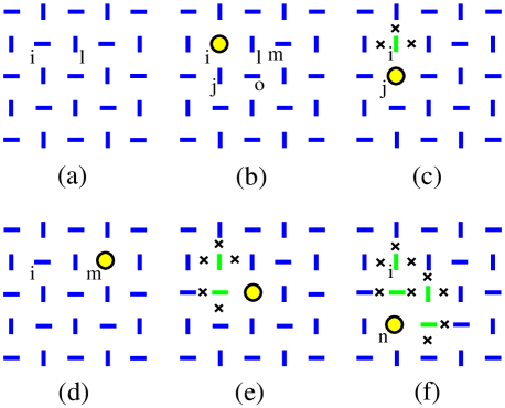
Figure 1: (Color online) Artist’s view of hole propagation in the ground state $|{\rm AO}\rangle$ with AO order presented in (a), with vertical (horizontal) bars standing for $a$ ($b$) occupied orbitals. (b) A hole doped into the physical vacuum $|{\rm AO}\rangle$ at site $i$ removes four exchange bonds. It can be shifted to new positions by consecutively applying different terms of the Hamiltonian: (c) a single NN hopping $t$, (d) a single three-site term $\tau$ (8), (e) a single three-site term $\tau$ (9), and (f) several steps which create more flipped orbitals; for more details see text. Broken bonds that cost the energy $\frac{1}{2}J$ each are marked by $\times$.

In contrast to this, the term (8) couples the states (b) and (d) without creating any defect in the orbital order. This term therefore enables true coherent motion in the insulating ground state with AO order.Woh08 Finally, the term (9) has yet another effect in that it connects the states (b) and (e), as well as the states (e) and (f). In other words this term connects string states whose number of defects differs by two. In some special cases the term (8) may ‘split off’ clusters of misaligned orbitals. Consider for example the state (f) and assume that the hole moves upward to site $i$ by virtue of hopping $\tau$ given by Eq. (8). Then a $2\times 2$ cluster of misaligned orbitals, all inverted with respect to the AO order, remains next to the hole in the final state.

In order to discuss the hole motion we restrict the Hilbert space to a basis of string states Brinkman_Rice ; Trugman ; Inoue_Maekawa ; Voijta_Becker which are created by successive application of ${\cal H}_{t}$ starting from the state (b). Unlike the case of a quantum antiferromagnet, the Hamiltonian (5) does not produce quantum fluctuations of the orbital order so that this restriction represents an even better approximation than in the spin $t$-$J$ model. Due to the directional nature of ${\cal H}_{t}$ and the orbital Néel order each hop along the string must be perpendicular to the preceding one so that the maximum number of different strings created after $n$ hops is $2^{n}$. The actual number of topologically different strings is less than this because one has to exclude self-intersecting paths. If we denote the sequence of sites visited by the hole by ${\cal F}=\{i_{0},i_{1},\dots i_{n}\}$ and introduce the ‘orbital-flip operator’ at site $i$,

$$\tilde{S}_{i}=c^{{\dagger}}_{i,\bar{o}(i)}\;c_{i,o(i)},$$ (11)

where $o(i)$ ($\bar{o}(i)$) denotes the orbital at site $i$ which is occupied (unoccupied) in the reference $|{\rm AO}\rangle$ state, the corresponding string state can be written as

$$|\Psi_{i,{\cal F}}\rangle=c_{i_{n},o(i_{n})}\;\prod_{j\in{\cal F}^{\prime}}\;\tilde{S}_{j}|{\rm AO}\rangle,$$ (12)

where it is understood that $i=i_{0}$ and ${\cal F}={\cal F}^{\prime}\cup\{i_{n}\}$. Since we want to study coherent hole motion, we construct Bloch states out of string states (12),

$$\left|\Psi_{{\bf k},{\cal S},{\cal F}}\right\rangle = \sqrt{\frac{2}{N}}\sum_{j}\;e^{i{\bf k}{\bf R}_{j}}\;T_{{\bf R}_{j}}|\Psi_{i,{\cal F}}\rangle,$$ (13)

$$\left|\Psi^{(n)}_{{\cal S},{\bf k}}\right\rangle = \sum_{{\cal F}}\;\alpha^{(n)}_{{\cal S},{\cal F},{\bf k}}|\Psi_{{\bf k},{\cal S},{\cal F}}\rangle.$$ (14)

Here we have introduced an additional sublattice index ${\cal S}\in\{{\cal{A}},{\cal{B}}\}$, whereby it is understood that $i\in{\cal S}$ and the sum over $j$ extends all translations of one sublattice. The coefficients $\{\alpha^{(n)}_{{\cal S},{\cal F},{\bf k}}\}$ are variational parameters and $n$ stands for a band index. An analogous ansatz for the related problem of a hole in a quantum antiferromagnet was used before in Refs. Trugman, ; Inoue_Maekawa, ; Voijta_Becker, . In practice, all different sets ${\cal F}$ up to a maximum number $n_{max}$ of defects are generated by computer and the Hamiltonian matrix is set up.

We have used $n_{max}=10$ and verified that the results for the low energy bands are well converged with respect to $n_{max}$. The matrix elements of the Hamiltonian for the pairs of states $\{$(b),(c)$\}$, $\{$(b),(d)$\}$ and $\{$(b),(e)$\}$ are $t$, $\tau$, and $-\tau$ respectively. The sign change with respect to the Hamiltonian (5) follows from the transformation of hopping terms to the hole picture. Due to the directional nature of the hopping terms the resulting band structure depends on the sublattice index ${\cal S}$.

Figure 2: Numerical results obtained for 20 bands with lowest energies, formed by propagating eigenstates $|\Psi^{(n)}_{{\cal B},{\bf k}}\rangle$: (a) energy dispersions along the (0,1) direction in the 2D Brillouin zone, and (b) the spectral function (15) for representative values of $k_{b}$. Parameters: $J=0.4t$, $\tau=0.1t$, $\delta=0.02t$.

Fig. 2(a) shows the dispersion of the lowest bands, $\epsilon_{b,n}({\bf k})$ as a function of $k_{b}$, where ${\bf k}=(0,k_{b})$ is the vector from the 2D Brillouin zone. The bands are obtained for hole doping at ${\cal B}$ sublattice and for representative parameters: Woh08 $J=0.4t$, $\tau=0.1t$. The energy of the AO state with no holes, shown in Fig. 1(a), has been used as the reference energy. In agreement with the 1D nature of the three-site effective hopping (8), the dispersion of the lowest energy state and of some excited states shows only dependence on $k_{b}$.

Figure 2(b) shows the single-particle spectral function, defined as

$$A({\bf k},\omega) = -\frac{1}{\pi}\Im\;\sum_{n}\frac{Z_{n}({\bf k})}{\omega-\epsilon_{b,n}({\bf k})+i\delta}\,,$$ (15)

$$Z_{n}({\bf k}) = |\alpha^{(n)}_{{\cal B},{\cal F}_{0},{\bf k}}|^{2}\,,$$ (16)

where the string ${\cal F}_{0}$ corresponds to the state (b) in Fig. 1. In other words, this is just the weight of the bare hole in the wave function (14). As expected, the dispersionless bands in Fig. 2(a) have practically no spectral weight — as will be seen below, however, these bands give a dominant contribution to the optical conductivity.

The spectral weight of the lowest peak — which would form the quasiparticle band at finite doping — shows a weak ${\bf k}$-dependence which can be understood as follows: For momenta near the minimum (maximum) of the dispersion, the hole gains (looses) energy by propagation. Since the dominant mechanism of propagation is the hopping of the bare hole via the three-site hopping term (8) — see the transition between states in Fig. 1 from (b) to (d) — this gain (loss) in energy will be larger if the weight of the bare hole in the wave function is larger. The weight of the bare hole, however, also gives the spectral weight of the quasiparticle peak. Therefore the weight of the peak is larger (smaller) near the minimum (maximum) of the dispersion.

IV Optical conductivity

IV.1 Numerical analysis

In the next step we discuss the optical conductivity, which is defined as $\sigma_{\alpha}(\omega)=\sigma_{{\cal A},\alpha}(\omega)+\sigma_{{\cal B},\alpha}(\omega)$, with the conductivity for sublattice ${\cal S}\in\{{\cal A},{\cal B}\}$:

$$\sigma_{{\cal S},\alpha}(\omega) = \sum_{{\bf k}}\sum_{n=1}\;\frac{1}{\omega}\;\left|\left\langle\Psi^{(n)}_{{\cal S},{\bf k}}\right|j_{\alpha}\left|\Psi^{(0)}_{{\cal S},{\bf k}}\right\rangle\right|^{2}$$ (17)

$$\times n_{{\cal S}{{\bf k}}}\;\delta\{\omega-(\epsilon_{{\cal S}n}({\bf k})-\epsilon_{{\cal S}0}({\bf k}))\}.$$

Here $\alpha\in\{a,b\}$ denotes the direction of the current operator $j_{\alpha}$, $|\Psi^{(n)}_{{\cal S},{\bf k}}\rangle$ are the approximate single-hole eigenstates (14) and $\epsilon_{{\cal S}n}({\bf k})$ are the corresponding eigenvalues. The $n_{{\cal S}{\bf k}}$ denote the ground state occupation numbers of these states which we assume to be different from zero only for the lowest band labeled by $n=0$. For a given level of hole doping $x$ they are determined by adjusting the Fermi energy. This implies that we are assuming that for finite hole concentration the lowest band for each sublattice is filled according to the Pauli principle. This procedure is reasonable for low density of doped holes $x$.

We proceed to the discussion of the current operator $j_{\alpha}$ (for more clarity the index $\alpha$ is skipped below). For the original Hamiltonian (1) this is given by

$${\bf j}=it\sum_{\delta=\pm 1}\left(\delta\hat{\textbf{b}}\;c^{\dagger}_{i+\delta{\bf\hat{b}},a}c_{i,a}+\delta\hat{\textbf{a}}\;c^{\dagger}_{i+\delta{\bf\hat{a}},b}c_{i,b}\right).$$ (18)

At this point one has to bear in mind that the wave functions (14) are (approximate) eigenstates of the strong coupling Hamiltonian (5) rather than the original model Eq. (1). It is well known that in order to obtain consistent results for a system described by the original Hamiltonian (1) it is necessary to subject the operator in question — here the current operator — to the same canonical transformation (4) as the Hamiltonian itself. This property has been pointed out in the strong coupling expansion for the spin Hubbard model,Esk94 and we follow here this procedure.

The result of a similar calculation for the present orbital problem is the strong coupling current operator:

$$j_{t_{2g}}\! = {\cal P}\left(j_{t}+j_{\rm 3s}^{(l)}+j_{\rm 3s}^{(d)}\right){\cal P}+O\left(\frac{t^{3}}{U^{2}}\right),$$ (19)

$$j_{t}\! = -it\sum_{i}\left({\bf\hat{a}}\;{c}^{\dagger}_{i,b}{c}_{i+{\bf\hat{a}},b}+{\bf\hat{b}}\;{c}^{\dagger}_{i,a}{c}_{i+{\bf\hat{b}},a}-\mbox{H.c.}\right),$$ (20)

$$j_{\rm 3s}^{(l)}\! = -2{\bf\hat{a}}\;i\tau\sum_{i}\left({c}^{\dagger}_{i-{\bf\hat{a}},b}{n}_{i,a}{c}_{i+{\bf\hat{a}},b}-\mbox{H.c.}\right)$$ (21)

$$- 2{\bf\hat{b}}\;i\tau\sum_{i}\left({c}^{\dagger}_{i-{\bf\hat{b}},a}{n}_{i,b}{c}_{i+{\bf\hat{b}},a}-\mbox{H.c.}\right),$$

$$j_{\rm 3s}^{(d)}\! = \mp({\bf\hat{a}}-{\bf\hat{b}})i\tau\sum_{i}\left({c}^{\dagger}_{i\pm{\bf\hat{b}},a}{c}_{i,a}{c}^{\dagger}_{i,b}{c}_{i\pm{\bf\hat{a}},b}-\mbox{H.c.}\right)$$ (22)

$$\mp \!\!\!({\bf\hat{a}}+{\bf\hat{b}})i\tau\sum_{i}\left({c}^{\dagger}_{i\mp{\hat{b}},a}{c}_{i,a}{c}^{\dagger}_{i,b}{c}_{i\pm{\bf\hat{a}},b}-\mbox{H.c.}\right).$$

It is instructive to trace back the origin of nontrivial terms appearing in Eq. (19). The terms which are of order $t^{2}/U$ stem from processes during which double occupancies are created at the intermediate stage due to the NN hopping in Eq. (18) and later removed by terms in the operator ${\cal U}$ which are of order $t/U$ or vice versa. It turns out that the process during which an electron with $b$ orbital flavor moves from one site to its neighbor and back, see sites $i$ and $j$ in Fig. 1(a), does not contribute to the transformed current operator $j_{t_{2g}}$ due to the cancelation which originates from the sign dependence of the prefactor in Eq. (18) related to the hopping direction. Since there is no such dependence in the case of hopping term in the Hamiltonian (1), the mentioned process gives rise to the exchange term (7) in the effective Hamiltonian.

The above cancelation does not take place in the processes with transfer the hole by two lattice spacings. In the first process $b$ orbital moves horizontally, as from site $m$ to site $l$ in Fig. 1(b), followed by another hop in the same direction onto an empty (hole) site — this gives rise to the contribution (21) to the effective current. In a second process, another $b$ orbital moves horizontally, and another hole is created along the diagonal of a plaquette (not shown). Such processes give rise to the contribution (22) to the effective current. Now, in the same way as for terms in the current operator related with NN hopping (20), we may deduce the matrix element of the current operator for terms related with further hopping in the direction ${\hat{\textbf{a}}}$ (or ${\hat{\textbf{b}}}$). For the pairs of states shown in Figs. 1(b), 1(d) and in Figs. 1(b), 1(e), one finds the matrix elements $-2i\tau$ ($0$) and $i\tau$ ($-i\tau$), respectively.

The transformed current operator (19) is next used to compute matrix elements between string states. For example, we find that the matrix element for the ${\hat{\textbf{b}}}$ component of the current operator $j_{b}$ (19) between states shown in Fig. 1(b) and 1(c) is $it$. The hole shift occurs downwards. The overall sign of the matrix term is positive, as the string states (b) $c_{i,b}|{\rm AO}\rangle$, and (c) $c_{j,a}c^{{\dagger}}_{i,a}c_{i,b}|{\rm AO}\rangle$, are defined in the hole language which brings about an additional sign change with respect to the prefactor appearing in Eq. (18). The matrix element of $j_{a}$ for the same pair of states vanishes.

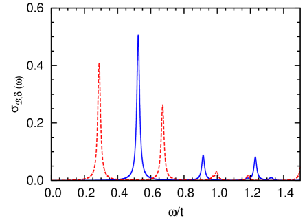
Figure 3: (Color online) Contribution to the optical conductivity $\sigma_{{\cal B}\delta}(\omega)$ measured along the $\delta={\hat{\textbf{a}}}$ (${\hat{\textbf{b}}}$) direction (solid line) and along the ${\hat{\textbf{b}}}$ (${\hat{\textbf{a}}}$) direction (dashed line), as obtained from transitions between states propagating along the ${\hat{\textbf{a}}}$ (${\hat{\textbf{b}}}$) direction at hole doping $x=0.1$. The total spectrum involving transitions from both kind of states is the sum of both contributions. Parameters: $J=0.4t$, $\tau=0.1t$. Lorentzian broadening of width $0.01t$ has been used.

The spectra of optical conductivity (17) (obtained by applying the Lorentzian broadening width of $0.01t$) are presented in Fig. 3. The solid line depicts the contribution to the conductivity measured along the $\delta={\hat{\textbf{a}}}$ direction from transitions between states propagating along the same direction, while the dashed line depicts the conductivity measured along the $\delta={\hat{\textbf{b}}}$ direction. The true response is the mixture of contributions from states propagating in both directions and for both $\delta={\hat{\textbf{a}}}$ and $\delta={\hat{\textbf{b}}}$. It is given by the superposition of the spectra plotted spectra in Fig. 3.

IV.2 Physical picture of transitions

Next we give a brief discussion of the physical significance of the optical transitions. In the discussion of hole motion we have seen that the dominant hopping term ${\cal H}_{t}$ does not lead to the coherent propagation of a hole because it creates a string of defects in the orbital order whence the energy increases linearly with the number of hops, i.e., with the string length. Coherent propagation is enabled only by the conditional NNN hopping term (8). Let us assume for the moment that this term is switched off. Then we can think of localized eigenstates of the remaining Hamiltonian

$$|\Psi_{i,\nu}\rangle=\sum_{{\cal F}}\;\alpha^{(\nu)}_{{\cal F}}|\Psi_{i,{\cal F}}\rangle.$$ (23)

There are several symmetry operations which transform the states $|\Psi_{i,\nu}\rangle$ into one another: inversion, rotation by $\pi$ and reflection by the $\hat{b}$ ($\hat{a}$) axis for $i\in{\cal A}$ ($i\in{\cal B}$). This corresponds to the symmetry group $C_{2v}$ and the local eigenstates (23) accordingly realize irreducible representations of this group. Next, the Bloch states (14) may alternatively be written as follows,

$$\left|\Psi^{(n)}_{{\cal S},{\bf k}}\right\rangle=\sum_{\nu}\;c_{\nu}^{(n)}|\Psi_{{\bf k},\nu}\rangle,$$ (24)

using the short-hand notation,

$$|\Psi_{{\bf k},\nu}\rangle=\sqrt{\frac{2}{N}}\sum_{j}\;e^{i{\bf k}{\bf R}_{j}}\;T_{{\bf R}_{j}}|\Psi_{i,\nu}\rangle.$$ (25)

This formulation — which is completely analogous to a local combination of atomic orbitals (LCAO) ansatz comprising $s$-like, $p$-like, $d$-like basis functions, etcetera — immediately clarifies the nature of the optical transitions: these are simply dipole-like transitions between the approximate local eigenstates $|\Psi_{i,\nu}\rangle$ generated by the interplay of hopping term ${\cal H}_{t}$ and the ‘string potential’. Since the current operator is e.g. odd under rotation by $\pi$, a matrix element $\langle\Psi_{i,\mu}|j_{\alpha}|\Psi_{i,\nu}\rangle$ is different from zero only if the two states, $|\Psi_{i,\mu}\rangle$ and $|\Psi_{i,\nu}\rangle$ have opposite parity. Since, moreover, the band with the lowest energy, $n=0$ in Eq. (14), has the totally symmetric ground state of the local Hamiltonian as its largest component, the peaks in the optical spectra give essentially — with only a small broadening due to weak dispersion — by the excitation energies of the states with odd parity. A very similar interpretation was also givenEde95 ; Voijta_Becker ; Plakida for the ‘mid infrared’ spectral weight observed in numerical studies of the spin $t$-$J$ modelSte90 and applies possibly to cuprate superconductors.

V Summary and conclusions

We have investigated the optical conductivity in the 2D orbital model as a generic model for studying orbital polarons in doped orbitally ordered ($t_{2g}$ or $p$) systems and capturing the essential physics. That effectively spinless model is applicable to planar systems like some transition metal oxides when (due to the tetragonal crystal field) degenerate $yz$ and $xz$ orbitals are active and singly occupied in a ferromagnetically ordered plane, or to cold atom systems in optical lattices when $p$ orbitals are active. It is demonstrated that in the presence of strong electron correlations, the tendency towards confinement determines the properties of the model, i.e., it can be viewed as a system of weakly coupled potential wells. The potential well physics originates from exchange energy increase induced by the sequences of orbitals flipped by a hole introduced by doping, when it moves in the orbitally ordered Mott insulator and generates a string potential along its path.

We have shown that propagating bands are much narrower in the present orbitally ordered system than in the spin $t$-$J$ model. Results of the analysis based on a variant of exact diagonalization, motivated by the string picture, suggest the formation of bands in the optical spectrum within the Mott-Hubbard gap, by analogy with the mid-infrared band observed in doped cuprates.Phi10 We predict that the optical conductivity would have this form in weakly doped Mott insulators with active orbital degrees of freedom, while at higher doping orbital stripes would form.Wro10 Similar to the spin dynamics of stripes in superconducting cuprates,Kru03 one expects qualitative changes in the optical conductivity for systems with domains of AO order separated by orbital stripes, which is an interesting topic for future studies. Other challenges are posed by orbital superfluidity in the $p$-band of a bipartite optical square lattice investigated recently,Wir11 or by spin-orbital systems, where an orbiton may separate from a spinon and propagate through a lattice as a distinct quasiparticle.Sch12

Appendix A Origin of optical transitions

The aim of this section is to analyze the mechanism underlying the doping induced formation of states lying within the Mott-Hubbard gap of a correlated insulator which is orbitally ordered. Furthermore, it will be discussed, how the structure of those states influences the optical response. We believe that despite some simplifications, conclusions which will be drawn from this analysis are applicable to more complex situations encountered in real systems revealing orbital order.

Due to the simplicity of the analyzed model the relevant part of the Hilbert space consists of states which can be obtained by subsequently shifting the hole created in the AO state, the situation shown in Fig. 1(b), to nearby sites. Thus we could use that original position of the hole — $\tilde{\bf R}({\bf R},{\cal F})$ [here $\tilde{\bf R}({\bf R},{\cal F})$ stands for the function of the present hole position ${\bf R}$ and the set of sites on which orbitals have been flipped (${\cal F}$)] to label a given string state $|\Psi_{{\bf R},{\cal F}}\rangle$. In order to determine $\tilde{\bf R}({\bf R},{\cal F})$ in a unique way, we additionally demand that the total length of hole path necessary to create the state $|\Psi_{{\bf R},{\cal F}}\rangle$ from a state representing a hole created at the site $\tilde{\bf R}({\bf R},{\cal F})$ in the AO state is minimal. For example, in the case of the state shown in Fig. 1(f) the vector ${\bf R}$ refers to the site $n$ while the vector $\tilde{\bf R}({\bf R},{\cal F})$ to the site $i$. In principle there could be more than one ”original site” obeying those conditions for a given pair $\{{\bf R}$, ${\cal F}\}$. In that case we would arbitrarily choose a single $\tilde{\bf R}({\bf R},{\cal F})$ and the new method of state labeling by the new pair $\{\tilde{\bf R}({\bf R},{\cal F}),{\cal F}\}$ would also work.

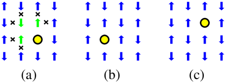
Figure 4: (Color online) The mechanism of the Trugman processTrugman allowing for hole deconfinement in a doped antiferromagnet described by the Ising model. (a) A hole doped to the Mott insulator with the antiferromagnetic order (spins are represented by arrows) generates six bonds with parallel spins by interchanging its position with spins on a plaquette after three hops. By a clockwise/anticlockwise hopping by three more steps one arrives at states (c)/(b), where all spin excitations are removed and the antiferromagnetic state is repaired — hence such processes couple the configurations (b) and (c). Broken bonds that cost the classical energy $\frac{1}{2}J$ each are marked by $\times$.

The possible ambiguity in determining the original position of the hole for a given string state would give rise to a new channel of coherent hole propagation which is known in the case of doped antiferromagnets. Fig. 4 depicts the so-called Trugman process Trugman which brings about hole deconfinement on a square lattice even in systems with Ising-type anisotropic exchange interaction as in the present orbital $t$-$J_{z}$ model. The state shown in Fig. 4(a) can be obtained both by shifting the hole clockwise or anticlockwise around the elementary plaquette by three lattice spacings (initially the hole replaced a $\downarrow$-spin as shown in Figs. 4(b) and 4(c), respectively). In other words, by performing one and a half of the circular movement of the hole on a given plaquette, the end effect is that the hole has moved along the plaquette diagonal without bringing about spin flips in the Néel state, which gives rise to the weak coherent hole propagation.

Now, with the help of the computer algebra, we will demonstrate that in the present two-orbital problem the ambiguity in determining the original position of the hole for a given string state does not exist in the case of a string state generated by a single hole, with a small number of twisted orbitals in the $|{\rm AO}\rangle$ state. Thus, it seems that the only channel allowing for hole propagation is due to the Hamiltonian induced coupling between states representing a hole created in the $|{\rm AO}\rangle$ state, as the states depicted in Figs. 1(b) and 1(d). This kind of hopping is mediated by the small $\tau\ll t$ term (8).

We proceed now to provide the justification of that statement when restricted to the low energy sector of the Hilbert space, i.e., consisting of states with limited number of flipped orbitals in the $|{\rm AO}\rangle$ state. The Hamiltonian matrix represented in terms of states $|\Psi_{{\cal S},{\cal F},{\bf k}}\rangle$ consists of two decoupled blocks. The first (second) block is formed by states coupled with the state representing a hole created in the perfect $|{\rm AO}\rangle$ state at a site belonging to the sublattice $\cal A$ ($\cal B$). Despite that both blocks show explicit dependence on both $\{k_{a},k_{b}\}$, the energies of eigenstates for each block disperse along a single direction, either (10) or (01) in the 2D Brillouin zone.

By representing the Hamiltonian matrix in terms of

$$|\tilde{\Psi}_{{\cal S},{\cal F},{\bf k}}\rangle=\sqrt{\frac{2}{N}}\sum_{i\in{\cal S}}e^{i{\bf k}\tilde{\bf R}({\bf R}_{i},{\cal F})}|\Psi_{{\bf R}_{i},{\cal F}}\rangle,$$ (26)

which is equivalent with performing a kind of gauge transformation, we get rid of the superfluous momentum dependence of the Hamiltonian matrix. Furthermore, if we neglect the term (8), the Hamiltonian matrix lacks any dependence on momentum, which shows that the hole deconfinement occurs here solely due to that term and that the hole becomes confined when $\tau$ is set to zero. Those findings are restricted to the basis considered by us which is limited by the path length. Furthermore, we do not probe the part of the Hilbert space which is not coupled by a Hamiltonian power to original states, representing a hole created in the $|{\rm AO}\rangle$ state. Thus, a general mathematical proof of the hypothesis regarding the nature of the propagation and valid for the whole Hilbert space is still needed.

To identify the origin of optical transitions contributing to the spectrum depicted in Fig. 3, we analyze now the properties of the Hamiltonian matrix represented in terms of states (26) [i.e., in the case when the original hole position is used to label string states], when $\tau$ is set to $0$, which means that only the “fast” part of the Hamiltonian is considered. It turns out that this part determines the overall structure of the energy-band hierarchy. Due to the lack of energy dispersion the bands are now completely flat, but their positions correspond very well to the sequence of bands obtained for finite $\tau$ and shown in Fig. 2. The picture which emerges from that correspondence is that the physics of hole hopping in the orbitally ordered background at large energy scale is determined by fast moves to NN sites, accompanied by the creation of defects in the orbital arrangement. Due to the increasing length of defect sequences (strings) a hole behaves like a particle in a potential well. Consequently, band hierarchy corresponds to the sequence of eigenenergies for the corresponding problem of the particle in the well. On the other hand, the energy dispersion is determined by “slow” hopping which brings about the modification at the energy scale $\sim\tau\ll t$ and can be viewed as a perturbation introduced on top of the robust structure of eigenstates arising for the potential-well problem. For finite $\tau$, the Hamiltonian matrix block formed by states coupled with the state representing a hole removed from the $\cal A$ ($\cal B$) sublattice in the $|{\rm AO}\rangle$ state does not show any dependence on $k_{a}$ ($k_{b}$), which explicitly demonstrates that the hole propagation is 1D.

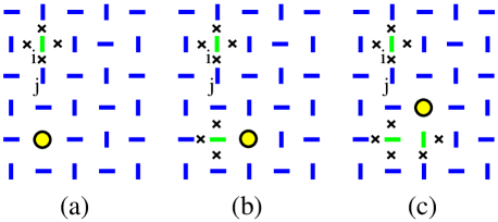
Figure 5: (Color online) Artist’s view of some disconnected string states which are not coupled by NN hopping $t$ with the original state of a hole doped in the AO state shown in Fig. 1(b). After moving by one hopping process $t$ from site $i$ to site $j$, the hole hops downwards by the effective hopping $\tau$ and leaves behind an island of excited bonds (a). Further hopping of the hole by either (b) one $t$ step, or (c) two $t$ steps, generates more defects in the $|{\rm AO}\rangle$ state. Broken bonds ($\times$) as in Fig. 4.

The point group of the underlying orbital background is $C_{2v}$. The Brillouin zone gets folded due to the staggered form of the AO order and all parameters like the energy are periodic with the periodicity $(\pi,\pi)$ and $(\pi,-\pi)$. The bottom of the lowest energy band lies on the lines $(\pi/2,k_{b})$ and $(k_{a},\pi/2)$ (and on lines equivalent by symmetry) for two orthogonal directions of the 1D hole propagation, respectively. Within the single particle approximation which we apply here, the Mott insulator doped with holes starts to fill orbital polaron bands near their bottoms. Even for nonzero $\tau$ the Hamiltonian blocks represented in the basis of states (26) are fully symmetric with respect to the point group $C_{2v}$ for wave vectors lying at the band bottom. For example, the block in the sector consisting of states lacking dispersion in the $\hat{\textbf{b}}$ direction is symmetric at the wave vector $(\pi/2,k_{b})$ with respect to the reflection in the $a$ axis, as it lacks the dependence on $k_{b}$. The inversion in the $b$ axis transforms $(\pi/2,k_{b})$ into $(-\pi/2,k_{b})$, which is the same as $(\pi/2,k_{b}+\pi)$ due to Brillouin zone folding, and equivalent to $(\pi/2,-k_{b})$ due to the lack of dependence on $k_{b}$. Thus we can use $C_{2v}$ to classify the symmetry properties of states at the band bottom.class

The ground state for both nonzero $\tau$ (system with propagating holes) and for $\tau$ set to zero (system with confined holes) is even with respect to both reflections: in the $a$ axis ($s_{a}$), and in the $b$ axis ($s_{b}$). In the latter case the states like the ones depicted in Figs. 5(a)-5(c) which are not coupled by a product of the $t$-hopping terms (6) with the original state, with a hole created in the $|{\rm AO}\rangle$ state at site $i$ and shown in Fig. 1(b), do not contribute to the ground state, while in the former case their weight is small. The state depicted in Fig. 5(a) is coupled with the state shown in Fig. 1(c) by the $\tau$-hopping term (8) which, on the other hand, is coupled with the original state presented in Fig. 1(b) by the $t$-hopping term (6). The states shown in Figs. 5(b) and 5(c) are both coupled by hopping terms with the state presented in Fig. 5(a).

The first excited state in the sector corresponding to the propagation in the $\hat{\textbf{a}}$ direction is odd with respect to the reflection $s_{a}$ and even with respect to $s_{b}$. Since the current operator (19) is an axial vector, its $b$ component (which is odd with respect to $s_{a}$) couples the first excited state with the fully symmetric ground state, which gives rise to the contribution to the optical weight in the form of the first peak from the left shown in Fig. 3. Upon doping, the optical transitions occur at momenta located in the vicinity of the band minimum, which explains why the peak gets a finite width. In the system with no propagating holes, the states such as those depicted in Fig. 5, which are not coupled by NN hopping to the original state, do not contribute to the first excited state, while their weight is small when the holes propagate.

References

- (1) S. Uchida, T. Ido, H. Takagi, T. Arima, Y. Tokura, and S. Tajima, Phys. Rev. B43, 7942 (1991).
- (2) A. Moreo and E. Dagotto, Phys. Rev. B 42, 4786 (1990).
- (3) W. Stephan and P. Horsch, Phys. Rev. B 42, 8736 (1990).
- (4) D. Poilblanc, T. Ziman, H. J. Schulz, and E. Dagotto, Phys. Rev. B 47, 14267 (1993).
- (5) J. Jaklič and P. Prelovšek, Phys. Rev. B50, 7129 (1994); 52, 6903 (1995).
- (6) R. Eder, Y. Ohta, and S. Maekawa, Phys. Rev. B51, 3265 (1995); R. Eder, P. Wróbel, and Y. Ohta, ibid. 54, R11034 (1996).
- (7) H. Eskes, M. B. J. Meinders, and G. A. Sawatzky, Phys. Rev. Lett. 67, 1035 (1991); M. B. J. Meinders, H. Eskes, and G. A. Sawatzky, Phys. Rev. B48, 3916 (1993).
- (8) H. Eskes and A. M. Oleś, Phys. Rev. Lett. 73, 1279 (1994); H. Eskes, A. M. Oleś, M. B. J. Meinders, and W. Stephan, Phys. Rev. B50, 17980 (1994).
- (9) Philip Phillips, Rev. Mod. Phys. 82, 1719 (2010).
- (10) Philip Phillips, Ting-Pong Choy, and Robert G. Leigh, Rep. Prog. Phys. 72, 036501 (2009).
- (11) D. Nicoletti, P. Di Pietro, O. Limaj, P. Calvani, U. Schade, S. Ono, Y. Ando, and S. Lupi, New J. Phys. 13, 123009 (2011).
- (12) X. Wang, H. T. Dang, and A. J. Millis, Phys. Rev. B84, 014530 (2011).
- (13) X. Zhang and E. Dagotto, Phys. Rev. B84, 132505 (2011).
- (14) Y. Tokura, Rep. Prog. Phys. 67, 797 (2006).
- (15) I. V. Solovyev, Phys. Rev. B63, 174406 (2001); M. Cuoco, C. Noce, and A. M. Oleś, ibid. 66, 094427 (2002).
- (16) N. N. Kovaleva, A. M. Oleś, A. M. Balbashov, A. Maljuk, D. N. Argyriou, G. Khaliullin, and B. Keimer, Phys. Rev. B81, 235130 (2010).
- (17) G. Khaliullin, P. Horsch, and A. M. Oleś, Phys. Rev. B70, 195103 (2004).
- (18) S. Miyasaka, Y. Okimoto, and Y. Tokura, J. Phys. Soc. Jpn. 71, 2086 (2002).
- (19) A. M. Oleś, J. Phys.: Condens. Matter 24, 313201 (2012).
- (20) Y. Okimoto, T. Katsufuji, T. Ishikawa, A. Urushibara, T. Arima, and Y. Tokura, Phys. Rev. Lett. 75, 109 (1995); Y. Okimoto, T. Katsufuji, T. Ishikawa, T. Arima, and Y. Tokura, Phys. Rev. B55, 4206 (1997).
- (21) A. M. Oleś and L. F. Feiner, Phys. Rev. B65, 052414 (2002); L. F. Feiner and A. M. Oleś, ibid. 71, 144422 (2005).
- (22) P. Horsch, J. Jaklič, and F. Mack, Phys. Rev. B59, 6217 (1999).
- (23) R. Kilian and G. Khaliullin, Phys. Rev. B60, 13458 (1999).
- (24) N. Pakhira, H. R. Krishnamurthy, and T. V. Ramakrishnan, Phys. Rev. B84, 085115 (2011).
- (25) J. Matsuno, Y. Okimoto, M. Kawasaki, and Y. Tokura, Phys. Rev. Lett. 95, 176404 (2005).
- (26) M. Hidaka, K. Inoue, I. Yamada, and P. J. Walker, Physica B & C 121, 343 (1983).
- (27) H. Wu and D. I. Khomskii, Phys. Rev. B76, 155115 (2007).
- (28) D. Jaksch and P. Zoller, Ann. Phys. (N.Y.) 315, 52 (2005).
- (29) X. Lu and E. Arrigoni, Phys. Rev. B79, 245109 (2009).
- (30) M. Daghofer, K. Wohlfeld, A. M. Oleś, E. Arrigoni, and P. Horsch, Phys. Rev. Lett. 100, 066403 (2008); K. Wohlfeld, M. Daghofer, A. M. Oleś, and P. Horsch, Phys. Rev. B78, 214423 (2008).
- (31) G. Khaliullin and S. Maekawa, Phys. Rev. Lett. 85, 3950 (2000); G. Khaliullin, P. Horsch, and A. M. Oleś, ibid. 86, 3879 (2001).
- (32) K. A. Chao, J. Spałek, and A. M. Oleś, J. Phys. C 10, L271 (1977); Phys. Rev. B18, 3453 (1978); A. M. Oleś, ibid. 41, 2562 (1990).
-
(33)
A. Wróbel and P. Wróbel,
Acta Phys. Polon. A 118, 409 (2010).
http://przyrbwn.icm.edu.pl/APP/ABSTR/118/a118-2-48.html - (34) This condition is fulfilled in transition metal oxides; here an effective interaction includes Hund’s exchange for the high-spin state, see also Ref. Woh08, .
- (35) W. F. Brinkman and T. M. Rice, Phys. Rev. B 2, 1324 (1970).
- (36) S. A. Trugman, Phys. Rev. B37, 1597 (1988); 41, 892 (1990).
- (37) J.-I. Inoue and S. Maekawa, J. Phys. Soc. Jpn. 59, 2110 (1990).
- (38) M. Vojta and K. W. Becker, Europhys. Lett. 38, 607 (1997); Eur. Phys. J. B 3, 427 (1998).
- (39) G. Jackeli and N. M. Plakida, Phys. Rev. B 60, 5266 (1999).
- (40) Piotr Wróbel and Andrzej M. Oleś, Phys. Rev. Lett. 104, 206401 (2010).
- (41) F. Krüger and S. Scheidl, Phys. Rev. B67, 134512 (2003).
- (42) G. Wirth, M. Olschlager, and A. Hemmerich, Nature Phys. 7, 147 (2011).
- (43) J. Schlappa, K. Wohlfeld, K. J. Zhou, M. Mourigal, M. W. Haverkort, V. N. Strocov, L. Hozoi, C. Monney, S. Nishimoto, S. Singh, A. Revcolevschi, J.-S. Caux, L. Patthey, H. M. Rønnow, J. van den Brink, and T. Schmitt, Nature 485, 82 (2012).
- (44) Strictly speaking, since the element of the point group transforms the states and into and , respectively, in the classification for the wavevector and we use and ; these states have the same matrix elements in the respective block for the Hamiltonian and the current operator as any term in the sum.