Subsurface Supergranular Vertical Flows as Measured Using Large Distance Separations in Time–Distance Helioseismology

Abstract

As large–distance rays (say, $10$ – $24^{\circ}$) approach the solar surface approximately vertically, travel times measured from surface pairs for these large separations are mostly sensitive to vertical flows, at least for shallow flows within a few Mm of the solar surface. All previous analyses of supergranulation have used smaller separations and have been hampered by the difficulty of separating the horizontal and vertical flow components. We find that the large separation travel times associated with supergranulation cannot be studied using the standard phase–speed filters of time–distance helioseismology. These filters, whose use is based upon a refractive model of the perturbations, reduce the resultant travel time signal by at least an order of magnitude at some distances. More effective filters are derived. Modeling suggests that the center–annulus travel time difference $[\delta t_{\rm{oi}}]$ in the separation range $\Delta=10$ – $24^{\circ}$ is insensitive to the horizontally diverging flow from the centers of the supergranules and should lead to a constant signal from the vertical flow. Our measurement of this quantity, $5.1\pm 0.1\rm{\,seconds}$, is constant over the distance range. This magnitude of signal cannot be caused by the level of upflow at cell centers seen at the photosphere of $10\rm{\,m\,s^{-1}}$ extended in depth. It requires the vertical flow to increase with depth. A simple Gaussian model of the increase with depth implies a peak upward flow of $240\rm{\,m\,s^{-1}}$ at a depth of $2.3\rm{\,Mm}$ and a peak horizontal flow of $700\rm{\,m\,s^{-1}}$ at a depth of $1.6\rm{\,Mm}$.

1 Introduction

S-Introduction

Supergranulation, first studied more than 50 years ago [Hart (1954), Leighton, Noyes, and Simon (1962)], continues to be an active area of research. A comprehensive review [Rieutord and Rincon (2010)] details the recent progress. It has proven difficult to measure the vertical flow of supergranules at the photospheric level. The recent measurements of a $10\rm{\,m\,s^{-1}}$ upflow at the center of the average cell with a horizontal variation consistent with a simple convection cell [Duvall and Birch (2010)] may have finally settled the issue. It is only through helioseismology that we would hope to measure the supergranulation flows below the photosphere. Duvall97 first showed that time–distance helioseismic techniques are sensitive to supergranules and that inversions to derive three–dimensional flow fields might be derived. However, Zhao03 showed that their ray–theory inversions could not separate the horizontal and vertical flows for a model flow field. The use of radial–order filters and Born approximation kernels has led to more successful separation [Jackiewicz, Gizon, and Birch (2008), Švanda et al. (2011)]. Gizon10 summarize the local helioseismic contributions to supergranulation.

An important quantity in time–distance helioseisomology is the arc separation $[\Delta]$ between pairs of photospheric locations whose signals are subsequently temporally cross correlated. Previous analyses used $\Delta$ less than $5^{\circ}$ ($61\rm{\,Mm}$) [Zhao and Kosovichev (2003)] or $2.4^{\circ}$ ($29.2\rm{\,Mm}$) [Jackiewicz, Gizon, and Birch (2008), Švanda et al. (2011)], as the sensitivity is greater for the horizontal flow, the signal–to–noise ratio is better for small separations, and basically no supergranulation signal could be seen at larger $\Delta$ in the travel time difference maps constructed from the relatively short (8–12 hours) time intervals required to study the one–day lifetime supergranules. In the present work, we show that the large separations of $\Delta=10$ – $24^{\circ}$ yield center–annulus travel time differences $[\delta t_{\rm{oi}}\equiv$ outward–going time minus inward–going time$]$ from the centers of average supergranules that are insensitive to the diverging horizontal flow and hence yield a purely vertical flow response.

In Section sec:1 the modeling efforts, including flow models that satisfy mass conservation, travel times computed from ray theory, and linear wave simulations through flow fields are presented. In Section sec:danal, the analysis of data is presented, and in Section sec:discuss the results are discussed.

2 Modeling

sec:1

2.1 Flow Model

sec:2.1 As our observational technique is to make averages about centers of supergranules, the flow model that we take is azimuthally symmetric and decays exponentially away from the cell center to simulate the effect of averaging a stochastic flow field. A time–independent flow is assumed with axisymmetry about the location of the average cell. A Cartesian coordinate system with $z$ positive upwards is defined. For these assumptions, the vanishing divergence of the mass flux implies

$$\frac{\partial}{\partial z}(\rho v_{z})=-\rho\bf{\nabla_{h}}\cdot\bf{v_{h}},\ilabel{eq:cont}$$ (1)

where $\rho$ is the $z$-dependent density, $v_{z}$ is the $z$-component of velocity, $\bf{\nabla_{h}}$ is the horizontal divergence, and $\bf{v_{h}}$ is the horizontal velocity. It is assumed that horizontal density variations can be ignored, as travel times are only weakly sensitive to density changes in the underlying medium [Hanasoge et al. (2012)]. The model is assumed to separate into horizontal and vertical functions

$${\bf{v_{h}}}\equiv-f(z){\bf{g}}(x,y),$$ (2)

$$v_{z}\equiv u(z)\bf{\nabla_{h}}\cdot\bf{g},$$ (3)

where ${\bf{g}}(x,y)$ is a vector in the horizontal plane with no units, $f(z)$ has units of velocity, and $u(z)$ has units of velocity times length. Our method of solution is to first specify the horizontal function ${\bf g}(x,y)$ and calculate its horizontal divergence $\bf{\nabla_{h}}\cdot\bf{g}$. The vertical function $u(z)$ is then specified, and Equation (eq:cont) is used to derive $f(z)$. Some straightforward algebra yields

$$f(z)=\frac{\partial u}{\partial z}+u(z)\frac{\partial\ln\rho}{\partial z}.$$ (4)

In general, models are considered with the horizontal function ${\bf{g}}(x,y)$ defined by

$${\bf{g}}(x,y)={\bf\hat{r}}J_{1}(kr)e^{-r/R},\ilabel{eq:gdef}$$ (5)

where ${\bf\hat{r}}$ is the outward radial unit vector in a cylindrical coordinate system, $J_{1}$ is the Bessel function of order one, $k$ is a wavenumber, $r$ is the horizontal distance from the origin, and $R$ is a decay length. $k$ and $R$ are, in principle, free parameters that will only have the default values $k=\frac{2\pi}{30}\rm{\,rad\,Mm^{-1}}$ and $R=15\rm{\,Mm}$ in this article. This type of horizontal variation was used by Birch07. This type of horizontal variation describes well the type of averaging of the supergranular field done in this paper, where one sees the outward flow as the first positive lobe of the $J_{1}$ function and on average, the inflow from the adjacent supergranular cells as the first negative range of the $J_{1}$ function.

In general, models have been considered with a Gaussian $z$-dependence. $v_{z}$ is specified at $r=0$ as a simple Gaussian:

$$v_{z}(r=0)=ku(z)=v_{0}e^{-(z-z_{0})^{2}/2\sigma_{z}^{2}},$$ (6)

where $z_{0}$ is the location of the peak of the vertical flow, $\sigma_{z}$ is the Gaussian sigma, and $v_{0}$ is the maximum vertical flow. To ultimately explain the large–distance travel times, the photosphere needs to be in the far tail of the Gaussian. As the upward flow at cell center is $10\rm{\,m\,s^{-1}}$ at the photosphere, this implies a considerably larger vertical flow at depth for the average cell. Values for these parameters that approximate the data are $v_{0}=240\rm{\,m\,s^{-1}}$, $z_{0}=-2.3\rm{\,Mm}$, and $\sigma_{z}=0.912\rm{\,Mm}$.

2.2 Ray Calculations

sec:rays

In the ray theory, the travel time difference for the two directions of propagation through a flow $\bf v$ is

$${\delta\tau}=-2\int_{\Gamma}\frac{{\bf v}\cdot{\bf{ds}}}{c^{2}},\ilabel{eq:tdif}$$ (7)

where $\Gamma$ is the ray path, $c$ is the sound speed, and ${\bf{ds}}$ is the element of length in

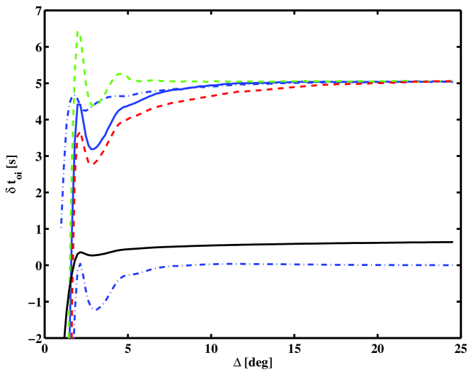
Figure 1.: Comparison of various ray models. The blue curves are for the Gaussian model with $z_{0}=-2.3\rm{\,Mm}$. The lower dot–dashed blue curve is for the horizontal flow component, the upper dot–dashed blue curve is for the vertical flow component and the solid blue curve is for the sum (upper solid curve). The upper dashed (green) curve is for the sum for $z_{0}=-1.15\rm{\,Mm}$ model and the lower dashed (red) curve is for the sum of the $z_{0}=-3.45\rm{\,Mm}$ model. The (lower) solid black curve is the sum for a model with a constant upflow of $10\rm{\,m\,s^{-1}}$. F-model1

the direction of the ray [Giles (2000)]. This equation naturally separates into two terms for the horizontal and vertical flow contributions to the travel time. The ray generation and raw ray integrations are performed using code developed and discussed in detail by Giles00. This code was extended to integrate quadrant and annulus surface–focusing integrations for 3D flow and sound speed perturbation models. In Figure F-model1 the black curve shows the travel time difference $[\delta t_{\rm{oi}}]$ for a flow model with a constant upflow of $10\rm{\,m\,s^{-1}}$. The black curve is for the sum of horizontal and vertical flows. That is, a horizontal flow of the form of Equation (eq:gdef) consistent through the continuity equation with a $10\rm{\,m\,s^{-1}}$ upflow is used. This signal, with a maximum of $0.6\rm{\,seconds}$, is much too small to explain the results derived in Section sec:gamma. This implies that the vertical flow must increase with depth from the photospheric value of $10\rm{\,m\,s^{-1}}$.

Also in Figure F-model1, the separate horizontal and vertical travel time contributions and the sum are shown for the Gaussian model mentioned above. For this relatively shallow model, it is seen that in the distance range $10$ – $24^{\circ}$, the signal is essentially constant and is mostly due to the vertical flow. Towards shorter distances, the horizontal flow contributes an increasing amount. The Gaussian model has three free parameters: $v_{0}$, $z_{0}$, and $\sigma_{z}$. In a later section the travel time difference for $10$ – $24^{\circ}$ will be determined to be $5.1\rm{\,s}$. This travel time difference and the $10\rm{\,m\,s^{-1}}$ upflow at the photosphere serve to determine two of the three free parameters. The travel time at $\Delta=24.5^{\circ}$ is forced to $5.1\rm{\,seconds}$. Letting $z_{0}$ be the free parameter, three models are plotted in Figure F-model1 with values of $z_{0}=-1.15\rm{\,Mm}$, $z_{0}=-2.30\rm{\,Mm}$, and $z_{0}=-3.45\rm{\,Mm}$. The shallowest model shows the least contribution from the horizontal component in the distance range $5$ – $10^{\circ}$. This distance range may supply a way to distinguish the best model while comparing with data.

A summary of the characteristics of these models is contained in Table T-models. The maximum vertical flow is at least a factor of 20 larger than the photospheric value. The ratio of the maximum horizontal flow to the photospheric value varies between four and eight. The maxima of the horizontal flow occurs somewhat shallower than the peak vertical flow.

Table 1.: Model details. The three models g1, g2, g3 are ones with Gaussian (g) upward flow at cell center peaking at $z0\rm{\,Mm}$ with peak flow $v_{z}(z0)\rm{\,m\,s^{-1}}$ and with Gaussian width $\sigma_{z}\rm{\,Mm}$. The upward flow at the top (z=0) is $v_{z}(0)\rm{\,m\,s^{-1}}$. The peak horizontal flow at the top is $v_{h}^{\rm{max}}(0)\rm{\,m\,s^{-1}}$ which occurs at radial distance $r^{\rm{\rm{max}}}\rm{\,Mm}$. The peak outward flow $v_{h}^{\rm{max}}\rm{\,m\,s^{-1}}$ occurs at $z(v_{h}^{\rm{max}})\rm{\,Mm}$. All of the maxima of $v_{h}$ occur at the same $r^{\rm{max}}$ by construction. The model sim1 is the one for the small features with just a z flow that are used for the flow perturbation described in Section sec:sim. T-models

Name	$z_{0}$	$\sigma_{z}$	$v_{z}(0)$	$v_{h}^{\rm{max}}(0)$	$r^{\rm{max}}$	$v_{z}(z0)$	$v_{h}^{\rm{max}}$	$z(v_{h}^{\rm{max}})$
g1	-3.45	1.39	10	122	7	218	460	-2.44
g2	-2.3	0.912	10	138	7	240	697	-1.62
g3	-1.15	0.433	10	195	7	340	1609	-0.83
sim1	-2.3	0.816	6.3			338

2.3 Simulation Results

sec:sim The applicability of ray theory to time–distance helioseismology has been called into question [Bogdan (1997)]. There are cases for supergranulation studies (Birch07, Figure 5) where it works reasonably well (amplitude of ray theory 25% higher than Born approximation kernels) and others where it is discrepant by a factor of two (Birch07, Figure 6). One case that works extremely well is the comparison of interior rotation determined from global modes and time–distance inversions (Giles00, Figure 6.2) in the radius range $0.89<r/R_{\odot}<0.999$. The difference between these cases seems to be that the ray theory works better when the spatial variation of the perturbation is larger, that is, much larger than the acoustic wavelength. One way to check the ray theory for a particular case is to compare with travel times computed from Born kernels [Birch and Gizon (2007)]. Another way to check is to perform simulations on a convectively–stabilized solar model with specified flow velocity perturbations and to propagate acoustic waves through the model [Hanasoge, Duvall, and Couvidat (2007)]. Travel times are computed from the simulations and then compared with ray–theory calculations of the travel times using the same flow velocity perturbations. This is the type of checking of the ray theory adopted here.

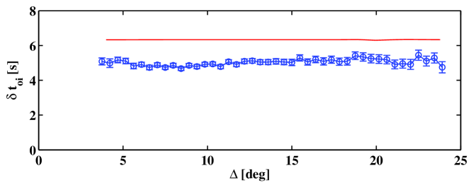
Figure 2.: Comparison of the center–annulus travel time differences $[\delta t_{\rm{oi}}]$ from the linear simulation (blue) with the travel–time difference computed from the ray theory with the same flow perturbations (red). The error bars are computed from the scatter far from the feature locations. No filtering has been done before the travel time measurements. The average travel–time difference in the range $\Delta=10$ – $24^{\circ}$ has been scaled to match the observationally determined mean $5.1\rm{\,seconds}$. The same scaling factor is then used to scale the ray theory results. In the range $\Delta=10$ – $24^{\circ}$, the ray theory predicts a travel–time difference too large by 24%. F-sim

A global simulation of wave propagation [Hanasoge and Duvall (2007)] with $768\times 384$ grid points in longitude and latitude respectively is performed over a ten–hour period. The flow perturbation consists of Gaussian features with a constant direction of vertical flow centered at a depth of $z_{0}=-2.30\rm{\,Mm}$ with $\sigma_{z}=0.82\rm{\,Mm}$ and with horizontal $\sigma_{h}=5.1\rm{\,Mm}$. There are 500 of these features placed at random longitude–latitude pairs at that depth $[z_{0}]$. Center–annulus travel time differences are measured from the simulation and averaged about the known locations. Realization noise is removed to first order by doing a similar simulation with no flow perturbation but with the same source excitations [Werne, Birch, and Julien (2004), Hanasoge, Duvall, and Couvidat (2007)] and subtracting the resultant $\delta t_{\rm{oi}}$ to obtain noise–corrected results.

The flow model that is inserted into the simulation is used with Equation (eq:tdif) to derive ray–theory predictions of the travel time differences. The results of the ray–theory computations and the travel time difference measurements from the simulation are shown in Figure F-sim. As the simulation only contains vertical flows, it is expected that there would be little or no variation of the travel–time differences with $\Delta$. The ray theory does predict too large a travel–time difference by 24%. This excess amplitude is similar to that found by Birch07. Although the amplitude computed from the ray theory is not precise, the necessity of large vertical flows to generate a travel–time difference of $5.1\rm{\,seconds}$ at $\Delta=10$ – $24^{\circ}$ is confirmed. The peak vertical flow for the normalized case is $338\rm{\,m\,s^{-1}}$. The model parameters are detailed in Table T-models.

3 Data Reduction and Analysis

sec:danal

3.1 Reduction

Dopplergrams from the Helioseismic and Magnetic Imager (HMI): [Schou et al. (2012)] onboard the Solar Dynamics Observatiory (SDO) spacecraft were analyzed for the present work. 32 days (10 June –  11 July 2010) of Dopplergrams were used to derive the final results, although a number of tests subsequently mentioned used only the last three days, 9 – 11 July 2010. This particular time period was used as the Sun was very quiet (sunspot number $RI\approx 15$ for these two months), and it was the final two–month continuous coverage period for the Michelson Doppler Imager (MDI) instrument [Scherrer et al. (1995)]. It might be useful to compare the results from the two instruments, but only the HMI data was used for the present study.

Raw Dopplergrams have a nine–day averaged Dopplergram subtracted as well as the spacecraft velocity which has a significant 24–hour component. These corrected Dopplergrams are remapped onto a coordinate system with equal spacing in latitude and longitude of $0.03^{\circ}$ covering a range of $144^{\circ}$ in both latitude and longitude. The remapping is achieved using a bilinear interpolation. The remapping in longitude is onto the Carrington system at a central longitude that crosses central meridian at the middle of the twelve–hour interval used. Two twelve–hour intervals are used for each day, covering the first and second halves of the day. Each remapped image is Fourier–filtered and resampled at $0.24^{\circ}$ per pixel. Twelve–hour datacubes are constructed from these individual images with $600\times 600$ spatial points and 960 temporal points for the $45\rm{\,s}$ sampling. This procedure works well for the large $\Delta$ emphasized in the present study, but would need to be modified to study smaller $\Delta$. Studying smaller $\Delta$ is deferred until future work.

The centers of the supergranules are located by a procedure used previously [Duvall and Birch (2010)]. The datacubes are spatio–temporally filtered to pass just the solar f–mode oscillations. Center–annulus travel time differences are computed [Duvall and Gizon (2000)] for the distance range $0.48$ – $1.02^{\circ}$. By using the difference of inward–going times minus outward–going times, the maps are equivalent to maps of the horizontal divergence. The equivalence of these maps to maps of supergranules has been shown before [Duvall and Gizon (2000), Duvall and Birch (2010)]. The travel–time difference maps are smoothed with a Gaussian of $\sigma=2.9\rm{\,Mm}$ to more easily determine the cell–center locations. Local maxima of this signal are picked as the cell centers. Lists of the locations are made. The one of a pair with the smaller divergence that are closer together $23\rm{\,Mm}$ is rejected. As it is desired to use center–annulus separations $\Delta<=25^{\circ}$, locations close to the edge of the maps are not used. On average, 930 features are located for each datacube with a total of 59549 for the 64 twelve–hour datasets. Overlays of cell–center locations with the divergence maps are shown in [Duvall and Birch (2010)].

3.2 Filtering

sec:filt Ray theory has proven invaluable in the development of time–distance helioseismology [Duvall et al. (1993)]. It led to the basic idea that signals propagating along ray paths between surface locations would lead to correlations between the temporal signals from which travel times could be inferred. As acoustic, or p, modes with the same horizontal phase speed $[\omega/k$: $\omega$ angular frequency and $k$ horizontal wavenumber$]$ travel along the same ray path to first order, it was natural to filter the data in $\omega/k$ to isolate waves traveling to a certain depth. This type of filter was introduced by Duvall93 with subsequent development by Kosovichev97 and Giles00. In the spatio–temporal power spectrum of solar oscillations ($k$–$\omega$ diagram), a line from the origin has a constant phase speed $\omega/k$. A range of phase speeds thus corresponds to a pie–shaped wedge. Phase–speed filtering then correponds to multiplying the Fourier transform of the input datacube by a pie–shaped wedge (appropriately modified for 3D) with some Gaussian tapering in phase speed [Couvidat and Birch (2006)].

Table 2.: Nominal phase speed filter parameters. The first column is an identification number. The second column is the range in distance $[\Delta]$. The third column is the mean distance $[\Delta_{\rm{mean}}]$. The fourth column is the central phase speed. The fifth column is the full width at half maximum (FWHM) of the Gaussian phase speed filter. For the tests in Section sec:filt, filters 1 – 13 were used while for the final results in Section sec:gamma, filters 1 – 14 were used. T-filtering

Filter	$\Delta[^{\circ}]$	$\Delta_{\rm{mean}}[^{\circ}]$	$v_{0}[\rm{\,km\,s^{-1}}]$	$\delta v[\rm{\,km\,s^{-1}}]$
1	1.56-2.28	1.92	32.0	13.2
2	2.28-3.00	2.64	41.8	4.2
3	3.00-3.96	3.48	46.9	6.0
4	3.96-4.92	4.44	54.7	9.5
5	4.92-6.12	5.52	64.5	10.1
6	6.12-7.80	6.96	75.1	11.1
7	7.56-9.24	8.40	84.3	10.4
8	9.12-10.7	9.84	93.5	9.4
9	10.92-12.60	11.76	104.4	9.7
10	12.36-14.52	13.44	114.2	12.5
11	14.28-16.44	15.36	125.2	12.3
12	17.16-19.32	18.24	141.9	12.6
13	19.08-22.20	20.64	156.0	18.5
14	22.08-24.00	23.04	170.4	11.8

The overriding principle of the use of the phase–speed filter is that solar perturbations lead to refractive time changes for signals travelling along a ray path. That this model is deficient was shown nicely in the work of Couvidat06 in which an artificial signal was detected with different amplitude depending on the width $[\delta v]$ of the pie–shaped wedge. They concluded that the Born–approximation kernels [Birch and Kosovichev (2000)], which are derived based on a single scattering from solar perturbations, are more appropriate. A better way to think of the problem is to consider waves impinging on a perturbation which are subsequently scattered.

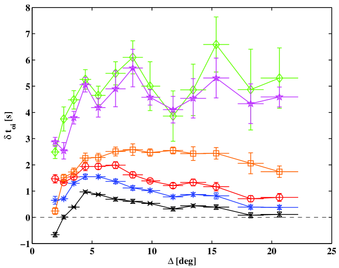
Figure 3.: Center–annulus travel time differences $[\delta t_{\rm{oi}}]$ averaged about the supergranule centers for different filters for the thirteen $\Delta$ ranges for three days of HMI data. From the bottom to top (on the right side), the black (x) points are for the the nominal phase–speed filters. The blue (*) points are for the phase–speed filters with the widths doubled. The red (o) points are for the width tripled. The orange (square) points are for a filter width that is half the nominal phase speed. The magenta (diamonds) curve is for the constant degree–width–filter (Section sec:gamma) with width $\Gamma_{\rm{\ell}}=400$. The green (pentagrams) curve is for no phase–speed filter. In all cases the f mode is excluded via filtering as is signal outside the frequency bandpass $1.5<\nu<6\rm{\,mHz}$. These results were obtained using the three days of data 9 – 11 July 2010. F-ph˙noph

An initial analysis was performed using some nominal phase–speed filters and distance ranges detailed in Table T-filtering. Thirteen distance ranges (and hence thirteen different filters) were applied to the six input datacubes for the dates 9 – 11 July 2010. The overall distance range covered for this test is $3.0$ – $22.2^{\circ}$. Center–annulus travel–time differences $[\delta t_{\rm{oi}}]$ were obtained for the thirteen distance ranges for each of the six datacubes using a standard surface–focusing time–distance analysis with the Gizon–Birch method of extracting travel times from the correlations [Gizon and Birch (2004)]. The travel times are averaged over the distance range and about the locations of the supergranular centers and the signal at the average cell center location is extracted. Uncertainties are estimated from the scatter of the six values. The travel–time differences are plotted versus $\Delta$ in Figure F-ph_noph (black). The variation with $\Delta$ does not agree with the models in Figure F-model1, but peaks near $\Delta=5^{\circ}$ and decays approximately to zero near $\Delta=20^{\circ}$.

There was some concern that this distance dependence might have something to do with the filtering, so a case was analyzed with no phase–speed filtering. The f mode was excluded and there was a frequency bandpass filter transmitting $\nu=1.5$ – $6\rm{\,mHz}$. The results of that analysis are also shown in Figure F-ph_noph (green). This shows a behavior with $\Delta$ much closer to the models in Figure F-model1 but with considerably more noise and a much larger signal close to five seconds. It was concluded that the phase speed filters were significantly degrading the signal. To test this further, the filters were broadened by the factors 2, 3, 4, 5 with the results of factors 2 (blue) and 3 (red) also shown in Figure F-ph_noph. More signal is obtained with the larger–width filters, but even with the factor of 5, only about 50% of the signal is obtained and there is still a decay of the signal towards larger $\Delta$.

Because of the approximate constancy of the simulation travel times $[\delta t_{\rm{oi}}]$ with $\Delta$ in Section sec:sim and the approximate constancy with $\Delta$ for the no phase–speed filter case, it was concluded that the decay of $\delta t_{\rm{oi}}$ toward larger $\Delta$ in the phase–speed filtered results is an artifact of the filtering. Filtering would seem to be desirable because of the large difference in errors for the unfiltered and filtered cases. But a filter is needed that gives a more unbiased result at the large $\Delta$ in order that the results not be overly dependent on the modeling. A first attempt at this was to use a set of filters with the full width at half maximum (FWHM) equal to half the phase speed [Birch et al. (2006)]. The results of these measurements are also shown in Figure F-ph_noph (orange). The dependence on $\Delta$ is somewhat reduced but there is still some decay at the largest $\Delta$.

A different way to look at this problem is to consider a p mode with frequency $\nu$ and spherical harmonic degree $\ell$ impinging on a supergranule. To the extent that the supergranule is static, the mode frequency $\nu$ will be maintained and the scattering will spread power in the spectrum away from the nominal value of $\ell$. The scattering should spread power over a width in $\ell$ that depends on the spectrum of supergranulation, which peaks near $\ell=120$. For similar values of the phase speed (which can also be characterized by $\nu/\ell$), the spread power should be over a similar width in $\ell$ [Chou et al. (1996), Woodard (2002)]. A filter that is centered at a certain phase speed but whose width is constant with $\nu$ and characterized by the FWHM in $\ell$ ($\equiv\Gamma_{\ell}$) may be what is needed. A value of $\Gamma_{\ell}=400$ should capture most of the supergranular signal. Such a filter was implemented and applied to the thirteen distance ranges used. The results are also shown in Figure F-ph_noph. The approximate constancy with $\Delta>5^{\circ}$ and the larger values than for the normal phase speed filters suggests that this type of filtering is a useful concept. The filter used has a flat top of width $\Gamma_{\ell}/2$ and is tapered to zero by a cosine bell that goes from 1 to 0 in $\Gamma_{\ell}/2$.

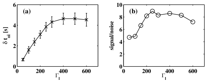
Figure 4.: (a) Travel–time difference $[\delta t_{\rm{oi}}]$ versus filter FWHM $[\Gamma_{\ell}]$. The unfiltered case has $5.3\pm 1.2\rm{\,seconds}$. (b) The travel time difference from (a) divided by the size of the error bar from (a) versus the filter FWHM $\Gamma_{\ell}$. The value for the unfiltered case is 4.6. F-tt˙and˙sn

Some additional tests of this new filter concept were computed. In Figure F-tt_and_sn(a) is shown the peak supergranular signal for $\Delta=19.08$ – $22.2^{\circ}$ as a function of the filter width $\Gamma_{\ell}$. For small $\Gamma_{\ell}$, much of the supergranular signal is removed, but as the width is increased more and more of the signal is transmitted. There is clearly a variation in the size of the error bars across Figure F-tt_and_sn(a). Another thing to examine is the ratio of the signal in Figure F-tt_and_sn(a) to the size of the error bar, which should give a value of the signal to noise ratio (S/N) of the filter [Couvidat and Birch (2006)]. This is plotted in Figure F-tt_and_sn(b). A rather broad peak is seen more or less centered on $\Gamma_{\ell}=400$. One noticeable aspect of Figure F-tt_and_sn(b) is that the unfiltered case gives a worse S/N (4.6) than the filters near the peak. Also narrow filters have reduced S/N. Based on the flatness of the $\Gamma_{\ell}=400$ results with $\Delta$ in Figure F-ph_noph, the extraction of essentially all the supergranular signal in Figure F-tt_and_sn(a), and the value of the S/N in Figure F-tt_and_sn(b), $\Gamma_{\ell}=400$ has been chosen for further analysis.

3.3 $\Gamma_{\ell}=400$ Analysis

sec:gamma The 64 twelve–hour datacubes were analyzed with the fourteen phase–speed filters with $\Gamma_{\ell}=400$. Center–annulus cross correlations were computed for the various distance ranges of Table 1. For checking purposes, it would be useful to be able to compute travel times using both the Gabor wavelet method [Duvall et al. (1997)] and the Gizon–Birch method [Gizon and Birch (2004)]. However, for the large distances in the present study ($\Delta<24^{\circ}$), individual twelve–hour cross correlations have insufficient signal–to–noise ratio to enable the Gabor wavelet fitting. It was decided to average the temporal correlations spatially about the supergranular centers. The averaging of the 930 (on average) correlations yields a high signal–to–noise ratio correlation that is amenable to the Gabor wavelet fitting at the largest distances $[\Delta]$. Averaging the resultant $\delta t_{\rm{oi}}$ for the 64 twelve–hour datacubes enables the use of the envelope–time differences $[t_{\rm{env}}]$ as well as the normal phase times $[t_{\rm{ph}}]$. Although most theoretical work applies to phase–time differences, it will be useful to examine the envelope–time differences as they may have independent information.

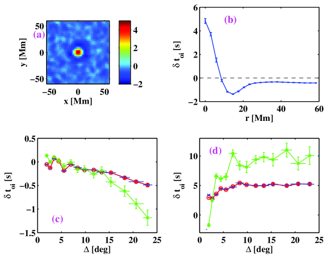
Figure 5.: (a) Center–annulus travel–time difference averaged about supergranule centers for the range of $\Delta=22.08$ – $24^{\circ}$. The scale of the colorbar at right is in seconds. Only the central point corresponding to the supergranular center is used in the present study. (b) Azimuthal average of (a). Note the offset at large radii. This offset is believed to be an artifact which needs to be removed from the results. (c) The offset at $r=58\rm{\,Mm}$ for the different travel–time definitions versus $\Delta$. Blue is for the Gabor wavelet phase time differences. Red is for the Gizon–Birch phase time differences and the green is for the Gabor wavelet envelope time differences. (d) The resultant travel time differences averaged for the 64 12–hour datacubes corrected for the offset in (c). The colors are the same as in (c). F-errplot

It was found previously that there is an offset from zero (of unknown origin) of the center–annulus travel–time differences [Duvall and Gizon (2000)]. For the small $\Delta$ of that study, the value of the offset was $0.16\pm 0.02\rm{\,seconds}$. This offset is assumed unrelated to the flows to be measured and needs to be removed from computed travel times. To measure it for the present study, the average maps about the supergranule centers for the 64 12–hour datacubes are computed for the different distance ranges. An example is shown for the largest range of $\Delta=22.08$ – $24^{\circ}$ in Figure F-errplot(a). An azimuthal average of Figure F-errplot(a) is computed and the result is shown in Figure F-errplot(b). At large radii $[r]$, the the signal is approximately constant. This constant, which is assumed to be the offset that needs to be subtracted from the results, is plotted for the various $\Delta$ and travel–time methods in Figure F-errplot(c). The Gizon–Birch and Gabor wavelet phase times yield almost exactly the same results, which is expected for the quiet Sun and the use of the same time window for fitting (20 minutes). The travel–time differences corrected for this offset are plotted in Figure F-errplot(d). Again, the Gizon–Birch and Gabor wavelet phase times yield almost precisely the same results with an average of $5.1\pm 0.1\rm{\,seconds}$ on the range $\Delta=10$ – $24^{\circ}$. The Gabor wavelet envelope times yield a considerbly larger value of $9.7\pm 0.3\rm{\,seconds}$ on $\Delta=10$ – $24^{\circ}$. In general the group velocity, $\partial\omega/\partial k$ is about one half of the phase speed $\omega/k$ for p modes, possibly leading to the larger travel time. The systematic error from Figure F-errplot(c) is generally less the 10% of the signal shown in Figure F-errplot(d).

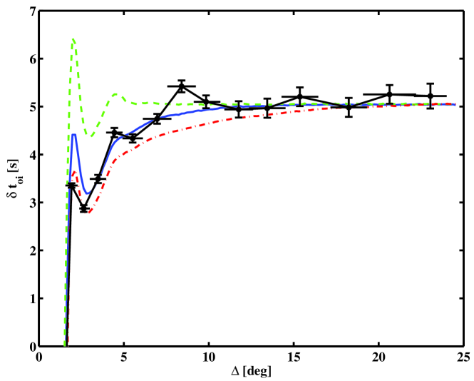
Figure 6.: Comparison of the three ray models from Figure F-model1 with the HMI results (black with symbols and errors) of the $\Gamma_{\ell}=400$ filtering and the Gabor–wavelet phase–speed time differences from Figure F-errplot(d). These models are the sum of vertical and horizontal signals for the three Gaussian vertical flows peaking at $z_{0}=-3.45\rm{\,Mm}$ (red dot–dashed), $z_{0}=-2.3\rm{\,Mm}$ (blue solid), and $z_{0}=-1.15\rm{\,Mm}$ (green dashed) specified in Table T-models. F-cmpplot

The Gabor–wavelet phase–time differences are plotted in Figure F-cmpplot versus the three ray models of Figure F-model1. The increase of the observed times for $\Delta=2.5$ – $8^{\circ}$ may be the effect of the horizontal flow. The agreement is a little better for the $z_{0}=-2.3\rm{\,Mm}$ model.

4 Discussion

sec:discuss The main observational result of this article is that in the distance range $\Delta=10$ – $24^{\circ}$ that the mean travel–time difference $[\delta t_{\rm{oi}}]$ at the center of the average supergranule is $5.1\pm 0.1\rm{\,seconds}$. How secure is this result? There are no other results to compare with in this distance range. Also, the method of averaging over many supergranules is uncommon [Birch et al. (2006), Duvall and Birch (2010), Švanda et al. (2011)]. The largest distance $[\Delta]$ used previously is $5^{\circ}$ by Zhao03. The phase–speed filter used in that study would have reduced the travel–time difference $[\delta t_{\rm{oi}}]$ by a factor of five and so it is difficult to compare. In addition, only inversions were presented and not raw travel–time differences.

One of the most interesting aspects of the present results is the large factor ($>20$) between the photospheric vertical flow and the peak vertical flow. This increase of vertical flow then also requires an increase of the horizontal flow from the photosphere to the peak of a factor between 3.7 and 8.3 from the simple Gaussian models g1 – g3. Some simple tests suggest that this horizontal velocity should be detectible by a quadrant time–distance analysis, which will be left for future work. Some previous analyses have detected some larger flows below the surface than at the surface [Duvall et al. (1997)]. Possibly the subsurface flow is highly variable which has made average properties difficult to ascertain from inversions of individual realizations.

These results confirm that supergranulation is a shallow phenomenon, with the flow peaking within a few Mm of the photosphere. This would tend to support models in which supergranulation is related to a near–surface phenomenon such as granulation [Rast (2003)]. The supergranular wave measurements [Gizon, Duvall, and Schou (2003), Schou (2003)], and in particular the variation with latitude of the anisotropy of wave amplitude, would suggest a connection with rotation. The near–surface shear layer has been modeled as a possible exciter of supergranulation [Green and Kosovichev (2006)]. Hathaway82 found that supergranulation as a convective phenomenon generates a near–surface shear layer. A difficulty with the near–surface shear layer as supergranular exciter is that recent simulations of Stein09 develop a near–surface shear layer but no hint of excess power at supergranular scales is seen.

Acknowledgements

The data used here are courtesy of NASA/SDO and the HMI Science Team. We thank the HMI team members for their hard work. This work is supported by NASA SDO and the NASA SDO Science Center program through grant SCEX22011D awarded to NASA GSFC. S. M. H. acknowledges funding from NASA grant NNX11AB63G.

References

- Birch et al. (2006) Birch, A., Duvall, T.L. Jr., Gizon, L., Jackiewicz, J.: 2006, Bull. of the Am. Astronom. Soc. 38, 224.
- Birch and Gizon (2007) Birch, A.C., Gizon, L.: 2007, Astronomische Nachrichten 328, 228.
- Birch and Kosovichev (2000) Birch, A.C., Kosovichev, A.G.: 2000, Solar Phys. 192, 193.
- Bogdan (1997) Bogdan, T.J.: 1997, Astrophys. J. 477, 475.
- Chou et al. (1996) Chou, D.-Y., Chou, H.-Y., Hsieh, Y.-C., Chen, C.-K.: 1996, Astrophys. J. 459, 792.
- Couvidat and Birch (2006) Couvidat, S., Birch, A.C.: 2006, Solar Phys. 237, 229.
- Duvall et al. (1993) Duvall, T.L. Jr., Jefferies, S.M., Harvey, J.W., Pomerantz, M.A.: 1993, Nature 362, 430.
- Duvall et al. (1997) Duvall, T.L. Jr., Kosovichev, A.G., Scherrer, P.H., Bogart, R.S., Bush, R.I., deForest, C., Hoeksema, J.T., Schou, J., Saba, J.L.R., Tarbell, T.D., Title, A.M., Wolfson, C.J., Milford, P.N.: 1997, Solar Phys. 170, 63.
- Duvall and Birch (2010) Duvall, T.L. Jr., Birch, A.C.: 2010, Astrophys. J. Lett. 725, L47.
- Duvall and Gizon (2000) Duvall, T.L. Jr., Gizon, L.: 2000, Solar Phys. 192, 177.
- Giles (2000) Giles, P.M.: 2000, Ph.D. Thesis, Stanford Univ.
- Gizon, Duvall, and Schou (2003) Gizon, L., Duvall, T.L. Jr., Schou, J.: 2003, Nature 421, 43.
- Gizon and Birch (2004) Gizon, L., Birch, A.C.: 2004, Astrophys. J. 614, 472.
- Gizon, Birch, and Spruit (2010) Gizon, L., Birch, A.C., Spruit, H.C.: 2010, Ann. Rev. of Astron. Astrophys. 48, 289.
- Green and Kosovichev (2006) Green, C.A., Kosovichev, A.G.: 2006, Astrophys. J. 641, L77.
- Hanasoge and Duvall (2007) Hanasoge, S.M., Duvall, T.L. Jr.: 2007, Astronomische Nachrichten 328, 319.
- Hanasoge, Duvall, and Couvidat (2007) Hanasoge, S.M., Duvall, T.L. Jr., Couvidat, S.: 2007, Astrophys. J. 664, 1234.
- Hanasoge et al. (2012) Hanasoge, S.M., Birch, A.C., Gizon, L., Tromp, J.: 2012, Phys. Rev. Letters (submitted).
- Hart (1954) Hart, A.B.: 1954, Mon. Not. Roy. Astron. Soc. 114, 17.
- Hathaway (1982) Hathaway, D.H.: 1982, Solar Phys. 77, 341.
- Jackiewicz, Gizon, and Birch (2008) Jackiewicz, J., Gizon, L., Birch, A.C.: 2008, Solar Phys. 251, 381.
- Kosovichev and Duvall (1997) Kosovichev, A.G., Duvall, T.L. Jr.: 1997, editors F.P. Pijpers, J. Christensen-Dalsgaard, and C.S. Rosenthal, SCORe’96 : Solar Convection and Oscillations and their Relationship 225, Kluwer, Dordrecht, 241.
- Leighton, Noyes, and Simon (1962) Leighton, R.B., Noyes, R.W., Simon, G.W.: 1962, Astrophys. J. 135, 474.
- Rast (2003) Rast, M.P.: 2003, Astrophys. J. 597, 1200.
- Rieutord and Rincon (2010) Rieutord, M., Rincon, F.: 2010, Liv. Rev. Sol. Phys. 7, 2.
- Scherrer et al. (1995) Scherrer, P.H., Bogart, R.S., Bush, R.I., Hoeksema, J.T., Kosovichev, A.G., Schou, J., Rosenberg, W., Springer, L., Tarbell, T.D., Title, A., Wolfson, C.J., Zayer, I., MDI Engineering Team: 1995, Solar Phys. 162, 129.
- Schou (2003) Schou, J.: 2003, Astrophys. J. Lett. 596, L259.
- Schou et al. (2012) Schou, J., Scherrer, P.H., Bush, R.I., Wachter, R., Couvidat, S., Rabello-Soares, M.C., Bogart, R.S., Hoeksema, J.T., Liu, Y., Duvall, T.L. Jr., Akin, D.J., Allard, B.A., Miles, J.W., Rairden, R., Shine, R.A., Tarbell, T.D., Title, A.M., Wolfson, C.J., Elmore, D.F., Norton, A.A., Tomczyk, S.: 2012, Solar Phys. 275, 229.
- Stein et al. (2009) Stein, R.F., Georgobiani, D., Schafenberger, W., Nordlund, Å., Benson, D.: 2009, AIP CS 1094, 764.
- Švanda et al. (2011) Švanda, M., Gizon, L., Hanasoge, S.M., Ustyugov, S.D.: 2011, Astron. Astroph. 530, A148.
- Werne, Birch, and Julien (2004) Werne, J., Birch, A., Julien, K.: 2004, editor: D. Danesy, In: SOHO 14 Helio- and Asteroseismology: Towards a Golden Future 559, ESA, Noordwijk, 172.
- Woodard (2002) Woodard, M.F.: 2002, Astrophys. J. 565, 634.
- Zhao and Kosovichev (2003) Zhao, J., Kosovichev, A.G.: 2003, Editor: H. Sawaya-Lacoste, In: GONG+ 2002. Local and Global Helioseismology: the Present and Future ESA SP-517, ESA, Noordwijk, 417.