Magnetized strange quark matter in a quasiparticle description

Abstract

The quasiparticle model is extended to investigate the properties of strange quark matter in a strong magnetic field at finite densities. For the density-dependent quark mass, self-consistent thermodynamic treatment is obtained with an additional effective bag parameter, which depends not only on the density but also on the magnetic field strength. The magnetic field makes strange quark matter more stable energetically when the magnetic field strength is less than a critical value of the order $10^{7}$ Gauss depending on the QCD scale $\Lambda$. Instead of being a monotonic function of the density for the QCD scale parameter $\Lambda>126$ MeV, the effective bag function has a maximum near $0.3\sim 0.4$ fm^-3. The influence of the magnetic field and the QCD scale parameter on the stiffness of the equation of state of the magnetized strange quark matter and the possible maximum mass of strange stars are discussed.

I Introduction

Since strange quark matter (SQM) was speculated by Witten as the possible true ground state of strong interaction matter witten , the properties of SQM in bulk, as well as in finite size, the so called strangelets, have been extensively studied in the past decades Farhi84 ; Buballa96 ; Madsen00 ; Dicus08 . The new form of matter is possibly produced by terrestrial relativistic heavy-ion collision experiments Heinz01 or exists in the interior of compact stars Alcock86 . It was found that the stability of SQM is strongly affected in a strong magnetic field Chakra1996 . The large magnetic fields in nature are normally associated with astrophysical objects, where the density is much higher than the nuclear saturation. The typical strength could be of the order $\sim 10^{12}$ G on the surface of pulsars Dong1991 . Some magnetars can have even larger magnetic fields, reaching the surface value as large as $10^{14}\sim 10^{15}$ G pacz . In the interior of compact stars, the maximum possible magnetic field strength is estimated as high as $\sim 10^{18}$ G. The origin of the strong magnetic fields can be understood in two ways. One is the amplification of the relatively small magnetic field during the star’s collapse with magnetic flux conservation Tatsumi06 . The other is the magnetohydrodynamic dynamo mechanism with large magnetic fields generated by rotating plasma of a protoneutron star Vink06 .

Because a strong magnetic field influences the single particle spectrum while all quarks are charged, SQM in the inner part of a compact star may show specific properties. Specially, for example, the strong magnetic field leads to a more stable polarized strange quark star (SQS)Bordbar11 . In heavy-ion collisions experiments, the magnitude of a magnetic field plays an important role in studying the deconfinement and chiral phase transitions. In the LHC/CERN energy, it is possible to produce a field as large as $5\times 10^{19}$ G Skokov09 .

With various phenomenological confinement models, many works on the properties of magnetized SQM(MSQM) have been done by a lot of researchers. Based on the conventional MIT bag model, quark matter in a strong magnetic field was studied by Chakrabarty Chakra1996 , and significant effect on the equation of state had been found. Furthermore, the magnetized strangelets at finite temperature was investigated by Felipe et. al. in their recent work Felipe ; Felipe2011 . In Ref. Mizher10 , the effect of an external magnetic field on the chiral dynamics and confining properties of SQM were discussed in the linear sigma model coupled to the Polyakov loops. The special properties of MSQM were also investigated with the Nambu-Jona-Lasinio (NJL) model Ebert03 ; Frol10 ; Faya11 ; Avan11 . The MIT bag model, the two-flavor NJL model, and the chiral sigma model had also been compared in studying the MSQM Rabhi2011 .

In literature, the quasiparticle model, where the effective quark mass varies with environment, was also successfully employed by many authors to study the dense strange quark matter in the absence of an external magnetic field vija95 ; Schertler1997 ; peshier2000 . The main advantage of the quasiparticle model is that it can explicitly describe quark confinement and vacuum energy density for bulk matter Schertler1997 and strangelets wen2010 . The aim of this article is to extend the quark quasiparticle model to studying the magnetized quark matter. We find a density- and magnetic-field-dependent bag function. Accordingly, a self-consistent thermodynamic treatment is obtained with the new version of the bag function. The effect of a magnetic field on the bag function and the stability of MSQM will be discussed. It is found that the magnetic field makes SQM more stable when the magnetic field strength is less than a critical value of the order $10^{7}$ G depending on the QCD scale $\Lambda$.

This paper is organized as follows. In Sec. 2, we derive the thermodynamic formulas in the quasiparticle model when the magnetic field becomes rather important, and then demonstrate the effective bag function for the case of both constant and running coupling, respectively. In Sec. 3, the stability properties of MSQM, the effective bag function, and the mass-radius relation of magnetized quark stars are investigated, and discussions are shown about the effect of the magnetic field and QCD scale parameter. The last section is a short summary.

II thermodynamic treatment in a strong magnetic field

The important feature of the quasiparticle model is the medium dependence of quark masses in describing QCD nonperturbative properties. The quasiparticle quark mass is derived at the zero-momentum limit of the dispersion relations from an effective quark propagator by resuming one-loop self-energy diagrams in the hard dense loop (HDL) approximation. In this paper, the effective quark mass is adopted as Schertler1997 ; Schertler1997jpg ; Pisarski1989

$$m_{i}(\mu_{i})=\frac{m_{i0}}{2}+\sqrt{\frac{m^{2}_{i0}}{4}+\frac{g^{2}\mu_{i}^{2}}{6\pi^{2}}}\,,$$ (1)

where $m_{i0}$ and $\mu_{i}$ are, respectively, the quark current mass and chemical potential of the quark flavor $i$. The constant $g$ is the strong interaction coupling. One can also use a running coupling constant $g(Q/\Lambda)$ in the equations of state of strange matter instead of a constant $g$ shir1997 . In our recent work by using phenomenological running coupling wen2010 , the quark masses were demonstrated to decrease with increasing densities at a proper region.

Here, we assume the $g$ value is in the range of $(0,0.5)$, as done in the previous work Schertler1997 . The current mass can be neglected for up and down quarks, while the strange quark current mass is taken to be $120$ MeV in the present calculations. Because the vanishing current mass is assumed for up and down quarks, Eq. (1) is reduced to the simple form

$$m_{i}=\frac{g\mu_{i}}{\sqrt{6}\pi}.$$ (2)

Instead of inserting the effective mass $m_{i}$ directly into the Fermi gas expression, we will derive the expressions from the self-consistency requirement of thermodynamics. The quasiparticle contribution of the flavor $i$ to the total thermodynamic potential density can be written as

$$\Omega_{i} = -\frac{d_{i}T}{(2\pi)^{3}}\int_{0}^{\infty}\left\{\ln\left[1+e^{-(\epsilon_{i,p}-\mu_{i})/T}\right]\right.$$ (3)

$$\phantom{-\frac{d_{i}T}{(2\pi)^{3}}\int_{0}^{\infty}\{}\left.+\ln\left[1+e^{-(\epsilon_{i,p}+\mu_{i})/T}\right]\right\}\mbox{d}^{3}\vec{p},$$

where $T$ is the system temperature and $d_{i}$ is the degeneracy factor [$d_{i}=3(\rm{color})$ for quarks and $d_{i}=1$ for electrons]. All the thermodynamic quantities can be derived from the characteristic function by obeying the self-consistent relation wen2009 .

To definitely describe the magnetic field of a compact star, we assume a constant magnetic field ($B_{m,z}=B_{m}$) along the $z$ axis. Due to the quantization of orbital motion of charged particles in the presence of a strong magnetic field, known as Landau diamagnetism, the single particle energy spectrum is Landau

$$\varepsilon_{i}=\sqrt{p_{z}^{2}+m_{i}^{2}+e_{i}B_{m}(2n+s+1)},$$ (4)

where $p_{z}$ is the component of particle momentum along the direction of the magnetic field $B_{m}$, $e_{i}$ is the absolute value of the electronic charge (e.g., $e_{i}=2/3$ for the up quark and 1/3 for the down and strange quarks), $n=0,1,2,...$, are the principal quantum numbers for the allowed Landau levels, and $s=\pm 1$ refers to quark spin-up and -down state, respectively. For the sake of convenience, we set $2\nu=2n+s+1$, where $\nu=0,1,2,...$. The single particle energy then becomes Chakra1996

$$\varepsilon_{i}=\sqrt{p_{z}^{2}+m_{i}^{2}+2\nu e_{i}B_{m}}.$$ (5)

On application of the quantized energy levels, the integration over $dp_{x}dp_{y}$ in Eq. (3) is replaced by the rule

$$\int_{-\infty}^{+\infty}\int_{-\infty}^{+\infty}dp_{x}dp_{y}\rightarrow 2\pi e_{i}B_{m}\sum_{s=\pm 1}\sum_{n}.$$ (6)

Because there is the single degenerate state for $\nu=0$ and the double degenerate state for $\nu\neq 0$, we assign the spin degeneracy factor ($2-\delta_{\nu 0}$) to the index $\nu$ Landau level. The thermodynamic potential density of Eq.(3) in the presence of a strong field can thus be written as

$$\Omega_{i}(T,m_{i},\mu_{i})=-T\frac{d_{i}e_{i}B_{m}}{2\pi^{2}}\sum_{v=0}(2-\delta_{\nu 0})\int_{0}^{\infty}\Big{\{}\ln[{1+\exp(\frac{\mu_{i}-\varepsilon_{i}}{T})}]+\ln[{1+\exp(\frac{-\mu_{i}-\varepsilon_{i}}{T})}]\Big{\}}dp_{z}.$$ (7)

At zero temperature, Eq. (7) is simplified to give

$$\Omega_{i}(m_{i},\mu_{i}) = -\frac{d_{i}e_{i}B_{m}}{2\pi^{2}}\sum_{v=0}(2-\delta_{\nu 0})\int_{0}^{\sqrt{\mu_{i}^{2}-M_{\nu}^{(i)2}}}(\mu_{i}-\varepsilon_{i})dp_{z}$$ (8)

$$= -\frac{d_{i}e_{i}B_{m}}{2\pi^{2}}\sum_{v=0}^{\nu_{max}}(2-\delta_{\nu 0})\Big{\{}\frac{1}{2}\mu_{i}\sqrt{\mu_{i}^{2}-M_{\nu}^{(i)2}}-\frac{1}{2}M_{\nu}^{(i)2}\ln(\frac{\mu_{i}+(\mu_{i}^{2}-{M_{\nu}^{(i)2}})^{1/2}}{M_{\nu}^{(i)}})\Big{\}},$$

where $M_{\nu}^{(i)}=\sqrt{m_{i}^{2}+2\nu e_{i}B_{m}}$ is the quark effective mass in the presence of a magnetic field. In the case of zero temperature, the upper limit $\nu_{max}$ of the summation index $\nu$ can be understood from the positive value requirement on the logarithm and square-root function in Eq. (8). So we have

$$\nu\leq\nu_{max}\equiv\mathrm{int}[\frac{\mu_{i}^{2}-m_{i}^{2}}{2e_{i}B_{m}}],$$ (9)

where “int” means the number before the decimal point.

Accordingly, the pressure $P$, the energy density $E$, and the free energy density $F$ for SQM at zero temperature read wen2005

$$P = -\Omega_{f}-B^{*},$$ (10)

$$E = F=\Omega_{f}+\sum_{i}\mu_{i}n_{i}+B^{*}.$$ (11)

Here $\Omega_{f}=\sum_{i}\Omega_{i}$ is the free quasiparticle contribution with the summation index going over all flavors considered. The notation $B^{*}$ denotes the effective bag function and it can be divided into two parts: $\mu_{i}$-dependent part and the definite integral constant part, i.e., $B^{*}=\sum_{i}B_{i}(\mu_{i})+B_{0}$ ($i=u$, $d$, and $s$) where $B_{0}$ is similar to the conventional bag constant and $B_{i}(\mu_{i})$ is the chemical potential dependent function to be determined.

The derivative of the thermodynamic potential density $\Omega_{i}$ with respect to the quark effective mass $m_{i}$ has an analytical expression, i.e.,

$$\frac{\partial\Omega_{i}}{\partial m_{i}}=\frac{\partial\Omega_{i}}{\partial M_{\nu}^{(i)}}\frac{\partial M_{\nu}^{(i)}}{\partial m_{i}}=\frac{d_{i}e_{i}B_{m}}{2\pi^{2}}\sum_{v=0}^{\nu_{max}}(2-\delta_{\nu 0})m_{i}\ln[\frac{\mu_{i}+(\mu_{i}^{2}-M_{\nu}^{(i)2})^{1/2}}{M_{\nu}^{(i)}}].$$ (12)

The quark particle number density of the component $i$ is given as

$$n_{i}=\frac{d_{i}e_{i}B_{m}}{2\pi^{2}}\sum_{\nu=0}^{\nu_{max}}(2-\delta_{\nu 0})\sqrt{\mu_{i}^{2}-M_{\nu}^{(i)2}}.$$ (13)

In the literature, there are three methods to construct a consistent set of thermodynamical functions with the effective quark masses. One is applied in the quark mass density-dependent model in Refs.Chakra91 ; peng99 , where all thermodynamic quantities are derived by direct explicit function and implicit function dependent relations. The second is the treatment in the NJL model, where the dynamical quark masses are solutions of the gap equation coupling the quark condensates buba99 ; Avan11 . The energy and pressure functions are modified accordingly. The third method is to get a self-consistent thermodynamical treatment with an effective bag constant to describe the residual interaction Romat03 . The effective bag constant acts as a part of a modified pressure function. Here, we employ the third method. The following requirement is introduced and applied as in Refs. Goren1995 ; Schertler1997 ,

$$\left(\frac{\partial P}{\partial m_{i}}\right)_{\mu_{i}}=0.$$ (14)

From a physical viewpoint, the constraint can make the formula of particle number function consistent with standard statistical mechanics. From Eqs. (10) and (11), it can be understood that the effective bag constant leads an additional term in the modification in the energy and pressure functions.

Considering Eq.(14), we have the vacuum energy density $B_{i}(\mu_{i})$ through the following differential equation

$$\frac{\mathrm{d}B_{i}(\mu_{i})}{\mathrm{d}\mu_{i}}\frac{\mathrm{d}\mu_{i}}{\mathrm{d}m_{i}}=-\frac{\partial\Omega_{f}}{\partial m_{i}}.$$ (15)

If we assume the vanishing current quark mass, one can integrate Eq. (15) under the condition $B_{i}(\mu_{i}=0)=0$ and have

$$B_{i}(\mu_{i}) = -\int^{\mu_{i}}_{0}\left.\frac{\partial\Omega_{f}}{\partial m^{*}_{i}}\right|_{T=0,\mu_{i}}\frac{\mathrm{d}m_{i}}{\mathrm{d}\mu_{i}}\mathrm{d}\mu_{i}$$ (16)

$$= -\frac{d_{i}e_{i}B_{m}}{2\pi^{2}}\sum_{\nu=0}^{\nu_{max}}(2-\delta_{\nu 0})\int_{\mu_{i}^{c}}^{\mu_{i}}\alpha^{2}\mu_{i}\ln(\frac{\mu_{i}+\sqrt{\mu_{i}^{2}-M_{\nu}^{(i)2}}}{M_{\nu}^{(i)}})d\mu_{i},$$

where the lower limit of the integration over $\mu_{i}$ is different from that in Ref. Schertler1997 . Its critical value $\mu_{i}^{c}$ should satisfy

$$\mu_{i}^{c2}-m_{i}^{2}-2\nu e_{i}B_{m}\geq 0$$ (17)

To reflect the asymptotic freedom of QCD, the calculation must be changed by including the running coupling constant. The approximate expression for the running quantity $g(\mu)$ reads Patra1996 ,

$$g^{2}(T=0,\mu)=\frac{48\pi^{2}}{29}\left[\ln(\frac{0.8\mu^{2}}{\Lambda^{2}})\right]^{-1},$$ (18)

where $\Lambda$ is the QCD scale parameter, the only free parameter in the theory determined by experiments. The magnitude of $\Lambda$ controls the rate at which QCD coupling constant runs as a function of exchanged momentum $Q^{2}$ (see Ref. shir1997 ). After applying the running coupling constant (18), the effective bag function in Eq. (16) is changed into

$$B_{i}(\mu_{i}) = -\int^{\mu_{i}}_{0}\left.\frac{\partial\Omega_{f}}{\partial m^{*}_{i}}\right|_{T=0,\mu_{i}}\frac{\mathrm{d}m_{i}}{\mathrm{d}\mu_{i}}\mathrm{d}\mu_{i}$$ (19)

$$= -\frac{d_{i}e_{i}B_{m}}{2\pi^{2}}\sum_{\nu=0}^{\nu_{max}}(2-\delta_{\nu 0})\int_{\mu_{i}^{c}}^{\mu_{i}}m_{i}\ln(\frac{\mu_{i}+\sqrt{\mu_{i}^{2}-M_{\nu}^{(i)2}}}{M_{\nu}^{(i)}})\frac{\mathrm{d}m_{i}(\mu_{i},g(\mu_{i}))}{\mathrm{d}\mu_{i}}d\mu_{i},$$

where the lower limit of the integration $\mu_{i}^{c}$ satisfies $B_{i}(\mu_{i}^{c}=0)$. Differently from the constant coupling case, the critical value $\mu_{i}^{c}$ can be obtained by inserting the running coupling constant in Eq. (18) into the condition (17). The value of $\mu_{i}^{c}$ depends not only on the chemical potential of quarks but also on the Landau energy level.

III properties of magnetized Strange quark matter

In this section, the properties of MSQM are studied with the new version of the quasiparticle model in the presence of a strong magnetic field. We will investigate the properties with a density- and magnetic-field-dependent bag function. Then, we discuss the effect of the QCD scale parameter and the strong magnetic field on the effective bag function and strange quark stars.

III.1 The stability property of bulk magnetized SQM

As is usually done, the SQM is treated as a mixture of $u$-, $d$-, $s$- quarks and electrons with neutrinos entering and leaving the system freely. To obtain the equations of state (EoS) of magnetized SQM, a set of equilibrium conditions–the weak equilibrium, baryon number conservation, and electric charge neutrality–should be considered by the following relations Chakra1996 ; band1997 ; Singh02 ; Gonz08 ; Felipe :

$$\mu_{u}+\mu_{e}=\mu_{d}=\mu_{s},$$ (20)

$$n_{u}+n_{d}+n_{s}=3n_{\mathrm{B}},$$ (21)

$$\frac{2}{3}n_{u}-\frac{1}{3}n_{d}-\frac{1}{3}n_{s}-n_{e}=0.$$ (22)

Equation (20) is the chemical equilibrium condition maintained by the weak-interaction processes such as $s+u\rightarrow u+d$ and $s\rightarrow u+e+\bar{\nu}_{e}$ etc., Eq. (21) is from the definition of the baryon number density $n_{\mathrm{B}}$, and Eq. (22) is the charge neutrality condition. For a given baryon number density $n_{\mathrm{B}}$, we can obtain the four chemical potentials $\mu_{u}$, $\mu_{d}$, $\mu_{s}$, and $\mu_{e}$ by solving the four equations in Eq. (20)-(22). Other thermodynamic quantities, such as the energy density and pressure, can then be calculated from the formulae derived in the previous section. A little difference is that the Maxwell contribution has been included in our numerical calculations, i.e., the quasiparticle contribution $\Omega_{f}$ is replaced by noron07 ; Mene09 ; Ferrer10

$$\Omega=\Omega_{f}+\frac{B_{m}^{2}}{2},$$ (23)

where the second term is the pure Maxwell contribution of the magnetic field itself.

In Fig. 1, the energy per baryon of MSQM is shown as functions of the density for several $g$ values. For comparison purposes, we have also plotted the previous results in Ref. wen2010 by setting $B_{m}=0$. The solid curves are for MSQM, while the dotted ones are for the corresponding nonmagnetized SQM. The two groups of curves have apparently similar density behavior. Obviously, however, the MSQM has lower energies than the nonmagnetized SQM. To show the effect of different coupling constants, we adopt three values of $g$.

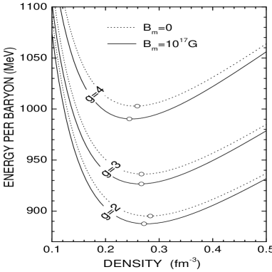
Figure 1: The energy per baryon versus the density at fixed coupling constant $g=2,3,4$ for magnetic field strength B${}_{m}=10^{17}$G. Compared with the nonmagnetized strange quark matter (the dotted curves with $B_{m}=0$), the magnetized case has a lower energy per baryon.

In the quasiparticle model, the parameter $g$ stands for the coupling strength and it is related to the strong interaction coupling constant $\alpha_{s}$ by $g=\sqrt{4\pi\alpha_{s}}$. Therefore, the g value has a large effect on the stability of SQM wen2011 . To satisfy the requirement of QCD asymptotic freedom, the running property of the coupling parametrization should be considered. In Fig. 2, we show the running coupling constant as functions of the baryon number density $n_{B}$. The three lines are obtained with different values of $\Lambda$. It is very obvious from Fig. 2 that the running coupling $g$ is a decreasing function of the density. With a bigger $\Lambda$ value, the coupling $g$ is also bigger at any fixed density.

Figure 2: The running coupling constant $g$ versus the baryon number density at different $\Lambda$ values with the magnetic field B${}_{m}=10^{17}$G. The upper lines correspond to larger values of $\Lambda$.

Figure 3: The energy per baryon $E/n_{B}$ of stable MSQM versus the number density at different $\Lambda$ values with the corresponding critical magnetic field strength B${}_{m}^{c}$.

In Fig. 3, we show the same quantities as in Fig, 1 with the running coupling constant, respectively for the two values of the different magnetic field $10^{17}$ G (dashed lines) and $10^{18}$G (solid lines). It is clearly seen that the energy per baryon increases with increasing the QCD scale parameter $\Lambda$, i.e. SQM has a lower energy per baryon with smaller $\Lambda$ value at a fixed strong magnetic field. This effect of the QCD scale parameter is consistent with the constant coupling case in Fig. 1, because larger $\Lambda$ means bigger coupling as indicated by Eq. (18).

An obvious observation from Fig. 3 is that there is a minimum energy per baryon for each pair of the parameters $\Lambda$ and $B_{m}$. In Fig. 4, therefore, we show how the minimum energy of MSQM varies with the magnetic field strength. The QCD scale parameter is taken to be 180 MeV (the upper dashed curve) and 120 MeV (the lower solid curve) respectively. It is found on each curve that there is another minimum value corresponding to a critical magnetic field strength $B_{m}^{c}$. For the values of $\Lambda=120$ MeV and $180$ MeV, the corresponding $B_{m}^{c}$ equals $2.15\times 10^{17}$ G and $2.34\times 10^{17}$ G respectively. When the magnetic field strength is less than $B_{m}^{c}$, the minimum energy per baryon decreases with increasing the strength of the magnetic field. When the magnetic field strength exceeds $B_{m}^{c}$, or, equivalently, when the magnetic energy scale approaches the QCD scale, i.e., $\sqrt{eB_{m}}\sim 76.9$ MeV, the field energy itself will have a considerable contribution to the energy of SQM and hence the energy per baryon increases with the magnetic field strength. In Fig. 3, the magnetic field strength is taken to be the corresponding critical value.

Figure 4: The energy of magnetized strange quark matter varies with the magnitude of the strong magnetic field for the fixed QCD scale parameter $\Lambda=180$ MeV (the upper dashed curve) and $\Lambda=120$ MeV (the lower solid curve) respectively. With decreasing the magnetic field strength, the energy per baryon approaches gradually to the value without a magnetic field indicated by a horizontal dashed-dotted line.

Because we study magnetized strange quark matter in the ”unpolarized” approximation, it is appropriate to estimate the maximum magnetic field strength when such an approximation can be reliable. To this end, in principle, we can investigate the polarized quarks with spin up (+) and down (-) by introducing the polarization parameter $\xi_{i}$ as Gonz08 ; Bordbar11

$$\xi_{i}=\frac{n_{i}^{(+)}-n_{i}^{(-)}}{n_{i}^{(+)}+n_{i}^{(-)}}.$$ (24)

where $n_{i}^{(+)}$ and $n_{i}^{(-)}$ denote the number density of spin-up and -down $i$-type quarks. For the sake of simplicity, we assume a common polarization rate $\xi$ for $u$-, $d$-, and $s$-quarks, i.e., $\xi_{\mathrm{u}}=\xi_{\mathrm{d}}=\xi_{\mathrm{s}}=\xi$. In Sec.II, the summation for fixed spin $s=+1$ or $s=-1$ should go over the principal quantum numbers $n$ instead of $\nu$. The degeneracy factor ($2-\delta_{\nu 0}$) in Eqs.(7), (8), (12) and (13) should be deleted because the spin degeneracy disappears for polarized particles. The polarization parameter $0\leq\xi\leq 1$ will decrease with increasing the number density. Assuming a larger value of the polarization $\xi=0.6$, the energy is enlarged by $4.5\%$. In fact, even for very larger magnetic field $B_{m}=5\times 10^{18}$G , the parameter $\xi$ remains in the range ($0.01\sim 0.02$) when the density $n_{B}>0.2$ fm ^-3 Bordbar11 . We do the numerical calculation and find that the free energy per baryon will be enlarged by $0.8\%$ at $\xi=0.1$. So the effect of the unpolarized approximation on the discussion of the stability of SQM is very small, especially when the magnetic strength is less than $10^{18}$G which is an estimated maximum possible strength of the interior magnetic field.

III.2 The effective bag function for magnetized SQM

The effective bag function $B^{*}$ is generally used to represent the vacuum energy density for dense QCD matter Agui03 . Comparing it with the standard statistical mechanics, one can recover the thermodynamics consistency of system density- and/or temperature-dependent Hamiltonian with the extra term $B^{*}$. The meaning of $B^{*}$ plays an important role in studying properties of quark matter. The interpretation of $B^{*}$ was first given by Gorenstein and Yang in Ref.Goren1995 . In quasiparticle model, because the dispersion relation is density- and/or temperature-dependent, $B^{*}$ is regarded as the system energy in the absence of quasiparticle excitations, which cannot be discarded from the energy spectrum Gardim07 . In this sense, $B^{*}$ acts as the bag energy or bag pressure through the application in bag-like model. One can interpret the confinement mechanism considering $B^{*}$ as the difference of perturbative vacuum and physical vacuum.

In addition to the constant value $B_{0}$ of the bag model, the expression of $B^{*}$ has been developed in several different forms. Li, Bhalerao, and Bhaduri obtained the temperature-dependent bag constant in the QCD sum-rule method Li91 . Song obtained a $\mu$- and $T$-dependent bag constant by incorporating one-loop correction in imaginary time formulation of finite temperature field theory Song92 ,

$$B^{*}(\mu,T)=B_{0}-[\frac{1}{162\pi^{2}}\mu^{4}+\frac{1}{9}\mu^{2}T^{2}+\frac{7\pi}{30}T^{4}].$$ (25)

In the work of Burgio Burgio02 , the Gaussian parametrization of density dependence of $B^{*}$ is employed as,

$$B^{*}(n_{B})=B_{\infty}+(B_{0}-B_{\infty})\exp(-\gamma(n_{B}/n_{0})^{2}),$$ (26)

where the parameters $B_{\infty}$, $\gamma$, and $n_{0}$ are given in Ref. Burgio02 . The effective bag constants in these previous works are all monotonically decreasing functions of the density and temperature Prasad04 . In our present work, the effective bag function $B^{*}$ is associated with a magnetic field and consequently has a different density behavior. We thus plot the effective bag function $B^{*}$ versus the baryon number density with different $\Lambda$ values in Fig. 5. The dashed lines are for the magnetic field strength $B_{m}=10^{17}$G, while the solid lines are for a higher magnetic strength $B_{m}=10^{18}$G. The open circles indicate nonmagnetized SQM. The numerical results show an important property that the effective bag function $B^{*}$ remains decreasing monotonously with increasing densities for smaller $\Lambda=120$ MeV. But for larger value $\Lambda=180$ or $200$ MeV, the bag function $B^{*}$ has a maximum value at about $2\sim 3$ times the nuclear saturation density $0.16$ fm^-3. Generally, when the QCD scale parameter is bigger than the critical value $126$ MeV, the effective bag function is not a monotonic function and reaches a maximum value $B^{*}_{\mathrm{max}}$ at the density range $0.3\sim 0.4$ fm^-3.

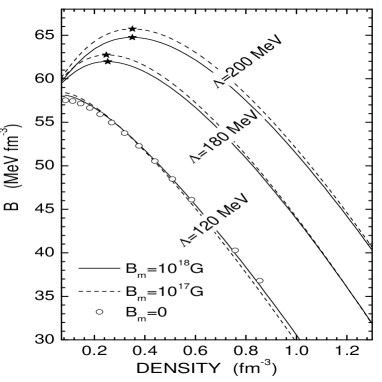
Figure 5: The effective bag function $B^{*}$ for MSQM versus the baryon number density at different $\Lambda$ values. $B_{m}=10^{17}$G and $B_{m}=10^{18}$G are marked by dashed lines and solid lines, respectively. Only for larger $\Lambda$, the $B^{*}$ has a maximum value $B^{*}_{\mathrm{max}}$ indicated by asterisks at $2\sim 3$ times nuclear saturation density.

Since the QCD scale parameter $\Lambda$ plays a great role on the effective bag function $B^{*}$, we plot the bag function $B^{*}$ of stable SQM, i.e., $P=0$, versus $\Lambda$ on the left axis in Fig, 6. If one requires that the bag function $B^{*}$ should be a nonmonotonic decreasing function of the density, the $\Lambda$ value should be bigger than the critical value $126$ MeV. The corresponding baryon number density $n_{B}$ marked by a dashed line on the right axis is also plotted. The bag function $B^{*}$ and the baryon number density $n_{B}$ all increase with the QCD parameter $\Lambda$.

Figure 6: $\Lambda$ dependence of the bag function $B^{*}$ (solid line) and baryon number density (dashed line) corresponding to the zero pressure. The $\Lambda$ should be larger than the critical value 126 MeV to produce a nonmonotonic behavior of $B^{*}$.

III.3 Mass-radius relation of magnetized strange quark stars

Strange quark stars, a family of compact stars consisting completely of deconfined $u$, $d$, $s$ quarks, have attracted a lot of researchers. The gravitational mass (M) and radius (R) of compact stars are of special interest in astrophysics. The strange quark stars were studied by many authors as self-bound stars different from neutron stars. It is pointed out that the possible configuration of compact stars, such as the strange hadrons, hyperonic matter, and quark matter core, can soften the equations of state of neutron stars Sahu2001 ; Shen2002 ; Burgio2002 . In this section, we calculate the mass-radius relation of magnetized SQS together with the effective quark mass scale. Using the EoS of MSQM in the proceeding sections, we can obtain M and R by numerically solving Tolman-Oppenheimer-Volkoff(TOV) equations when fixing a central pressure $P_{c}$. Varying continuously the central pressure, we can obtain a mass-radius relation $\textit{M(R})$ in Fig. 7. The stable branches of the curves must satisfy the condition $dM/dP_{c}>0$. In this way, we can find the maximum mass along the same curve, which is denoted by full dots in Fig. 7. Other solutions, on the left side of the maximum mass, are unstable and collapsible.

It is seen from Fig. 7 that the maximum mass is bigger with a smaller $\Lambda$ value and an extremely large magnetic field. However, it is still not as big as the recently observed maximum mass of PSR J1614-2230 Demo2010 . This may mean that a simple ordinary phase cannot explain the large mass. Some new phases, e.g., the superconductivity phase in dense matter wilczek01 ; Madsen01 ; Peng06 , should be further studied in the future.

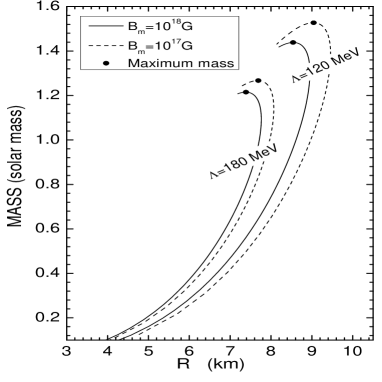
Figure 7: The mass-radius relation of SQS at different $\Lambda$ values with different magnetic fields B${}_{m}=10^{17}$G (dashed lines) and B${}_{m}=10^{18}$G (solid lines). The maximum masses on all curves are marked by full dots.

IV summary

We have extended the quark quasiparticle model to study the properties of strange quark matter in a strong magnetic field at finite density. The self-consistent thermodynamic treatment is obtained through an additional bag function. The bag function depends not only on the quark chemical potentials but also on the magnetic field strength $B_{m}$. By comparison with the nonmagnetized quark matter, we find that the magnetic field can enhance the stability of SQM when the magnetic field strength is lower than a critical value of the order $10^{17}$ G. But when the magnitude of the magnetic field is larger than the critical value $B_{m}^{c}$, the magnetic energy will have a considerable contribution to the energy of SQM. So the energy per baryon of MSQM increases with increasing the field strength. Because the quark masses depend on the corresponding chemical potential, an additional effective bag function, which depends not only on the chemical potentials but also on the magnetic field strength, appears in both the energy density and pressure. The effective bag function has a maximum at about $2\sim 3$ times the saturation density when the QCD scale parameter is larger than $126$ MeV. Although an unpolarized approximation is assumed, we find the energy per baryon would increase by $0.8\%$ for the usual polarization parameter when $n_{B}>0.2$ fm^-3.

On application of the new equation of state of the magnetized strange quark matter in ordinary phase to calculate the mass-radius relation of a quark star, it is found that the maximum mass does not explain the the newly observed maximum mass of about two times the solar mass. This means that other phases, e.g. superconductivity and/or mixed phases, might be necessary to explain the new astronomic observations, and further studies are needed.

- (1) E. Witten, Phys. Rev. D 30, 272 (1984).
- (2) E. Farhi and R. L. Jaffe, Phys. Rev. D 30, 2379 (1984).
- (3) M. Buballa, Nucl. Phys. A611, 393 (1996).
- (4) J. Madsen, Phys. Rev. Lett. 85, 4687 (2000).
- (5) D. A. Dicus, W. W. Repko, and V. L. Teplitz, Phys. Rev. D 78, 094006 (2008).
- (6) U. Heinz, Nucl. Phys. A685, 414c (2001).
- (7) C. Alcock, E. Farhi, and A. Olinto, Astrophys. J. 310 261 (1986).
- (8) S. Chakrabarty, Phys. Rev. D 54, 1306 (1996).
- (9) L. Dong and S. L.Shapiro, Astrophys. J. 383, 745 (1991).
- (10) B. Paczynski, Acta Astron. 42, 145 (1992); C. Thompson and R. C. Duncan, Astrophys. J. 392, L9 (1992).
- (11) T. Tatsumi, T. Maruyama, E. Nakano, and K. Nawa, Nucl. Phys. A774, 827 (2006).
- (12) J. Vink and Ll. Kuiper, Mon. Not. R. Astron. Soc. Lett. 370 L14 (2006).
- (13) G. H. Bordbar, and A. R. Peivand, Res. Astron. Astrophys. 11, 851 (2011).
- (14) V. Skokov, A. Illarionov, and V. Toneev, Int. J. Mod. Phys. A 24, 5925 (2009).
- (15) R. González Felipe and A. Pérez martínez, J. Phys. G 36, 075202 (2009).
- (16) R. González Felipe, E. López Fune, D. Manreza Paret, and A. Pérez Martínez, J. Phys. G 39, 045006 (2012).
- (17) A. J. Mizher, and M. N. Chernodub, and E. S.Fraga, Phys. Rev. D 82, 105016 (2010).
- (18) D. Ebert and K. G. Klimenko, Nucl. Phys. A728, 203 (2003).
- (19) I. E. Frolov, V. C. Zhukovsky, and K. G. Klimenko, Phys. Rev. D 82, 076002 (2010).
- (20) S. Fayazbakhsh, and N. Sadooghi, Phys. Rev. D 83, 025026 (2011).
- (21) D. P. Menezes, M. Benghi Pinto, S. S. Avancini, and C. Providência, Phys. Rev. C 80, 065805 (2009); S. S. Avancini, D. P. Menezes, and C. Providência, Phys. Rev. C 83, 065805 (2011).
- (22) A. Rabhi and C. Providência, Phys. Rev. C 83, 055801 (2011).
- (23) H. Vija and M. H. Thoma, Phys. Lett. B 342, 212 (1995).
- (24) K. Schertler, C. Greiner and M. H. Thoma, Nucl. Phys. A616, 659 (1997).
- (25) A. Peshier, B. Kämpfer, and G. Soff, Phys. Rev. C 61, 045203 (2000).
- (26) X. J. Wen, J. Y. Li, J. Q. Liang, and G. X. Peng, Phys. Rev. C 82, 025809 (2010).
- (27) R. D. Pisarski, Nucl. Phys. A498, 423c (1989).
- (28) K. Schertler, C. Greiner and M. H. Thoma, J. Phys. G 23, 2051 (1997).
- (29) D. V. Shirkov and I. L. Solovtsov, Phys. Rev. Lett. 79, 1209 (1997).
- (30) X. J. Wen, Z. Q. Feng, N. Li, and G. X. Peng, J. Phys. G 36, 025011 (2009).
- (31) L. D. Landau and E. M. Lifshitz, Quantum Mechanics (Pergamon Press, New York, 1965).
- (32) X. J. Wen, X. H. Zhong, G. X. Peng, P. N. Shen, and P. Z. Ning, Phys. Rev. C 72, 015204 (2005).
- (33) S. Chakrabarty, Phys. Rev. D 43, 627 (1991).
- (34) G. X. Peng, H. C. Chiang, J. J. Yang, L. Li, and B. Liu, Phys. Rev. C 61, 015201 (1999).
- (35) M. Buballa and M. Oertel, Phys. Lett. B 457, 261 (1999); M. Baldo, G. F. Burgio, P. Castorina, S. Plumari, and D. Zappalà, Phys. Rev. C 75, 035804 (2007).
- (36) P. Romatschke, arXiv:hep-ph/0312152.
- (37) M. I. Gorenstein and S. N. Yang, Phys. Rev. D 52, 5206 (1995); N. Prasad and C. P. Singh, Phys. Lett. B 501, 92 (2001).
- (38) B. K. Patra and C. P. Singh, Phys. Rev. D 54, 3551 (1996).
- (39) D. Bandyopadhyay, S. Chakrabarty, and S. Pal, Phys. Rev. Lett. 79, 2176 (1997).
- (40) S. Singh, N. C. Devi, V. K. Gupta, A. Gupta, and J. D. Anand, J. Phys. G 28, 2525 (2002)
- (41) R. G. Felipe, A. P. Martínez, H. P. Rojas, and M. Orsaria, Phys. Rev. C 77, 015807 (2008).
- (42) J. L. Noronha and I. A. Shovkovy, Phys. Rev. D 76, 105030 (2007).
- (43) D. P. Menezes, M. B. Pinto, S. S. Avancini, A. P. Martínez, and C. Providência, Phys. Rev. C 79, 035807 (2009).
- (44) E. J. Ferrer, V. de la Incera, J. P. Keith, I. Portillo, and P. L. Springsteen, Phys. Rev. C 82, 065802 (2010); L. Paulucci, E. J. Ferrer, V. de la Incera, and J. E. Horvath, Phys. Rev. D 83, 043009 (2011).
- (45) X. J. Wen, D. H. Yang, and S. Z. Su, J. Phys. G 38, 115001 (2011).
- (46) R. Aguirre, Phys. Lett. B 559, 207 (2003).
- (47) F. G. Gardim and F. M. Steffens, Nucl. Phys. A797, 50 (2007).
- (48) S. Li, R. S. Bhalerao, and R. K. Bhaduri, Int. J. Mod. Phys A 6, 501 (1991).
- (49) G. Song, W. Ewke, and L. Jiarong, Phys. Rev. D 46, 3211 (1992).
- (50) G. F. Burgio, M. Baldo, P.K. Sahu, A.B. Santra, H.-J. Schulze, Phys. Lett. B 526, 19 (2002).
- (51) N. Prasad and R. S. Bhalerao, Phys. Rev. D 69, 103001 (2004).
- (52) P. K. Sahu, and A. Ohnishi, Nucl. Phys. A691, 439 (2001).
- (53) H. Shen, Phys. Rev. C 65, 035802 (2002); F. Yang and H. Shen, Phys. Rev. C 77, 025801 (2008).
- (54) G. F. Burgio, M. Baldo, P. K. Sahu, and H. J. Schulze, Phys. Rev. C 66, 025802 (2002).
- (55) P. Demorest, T. Pennucci, S. Ransom, M. Roberts, and J. Hessels, Nature 467, 1081 (2010)
- (56) K. Rajagopal and F. Wilczek, Phys. Rev. Lett. 86, 3492 (2001).
- (57) J. Madsen, Phys. Rev. Lett. 87, 172003 (2001).
- (58) G. X. Peng, X. J. Wen and Y. D. Chen, Phys. Lett. B 633, 314 (2006).