Fokker-Planck equation with memory: the crossover from ballistic to diffusive processes in many-particle systems and incompressible media

Abstract

The unified description of diffusion processes that cross over from a ballistic behavior at short times to normal or anomalous diffusion (sub- or superdiffusion) at longer times is constructed on the basis of a non-Markovian generalization of the Fokker-Planck equation. The necessary non-Markovian kinetic coefficients are determined by the observable quantities (mean- and mean square displacements). Solutions of the non-Markovian equation describing diffusive processes in the physical space are obtained. For long times, these solutions agree with the predictions of the continuous random walk theory; they are, however, much superior at shorter times when the effect of the ballistic behavior is crucial.

Key words: non-Markovian processes, fractional diffusion, ballistic effects

PACS: 05.40 Fb, 05.40 Jc, 51.10 +y

Abstract

На основi немаркiвського узагальнення рiвняння Фокера-Планка запропоновано пiдхiд до об’єднаного опису дифузiйних процесiв, який дозволяє розглядати як балiстичний режим на малих часах, так i аномальну (суб- або супер-) дифузiю на великих часових iнтервалах. Встановлено зв’язок немаркiвських кiнетичних коефiцiєнтiв зi спостережуваними величинами (середiми та середньоквадратичними змiщеннями). Отримано розв’язки, що описують дифузiйнi процеси у фiзичному просторi. Для великих часiв еволюцiї вони узгоджуються з результатами теорiї неперервних в часi випадкових блукань, а на малих часах описують балiстичну динамiку.

Ключовi слова: немаркiвськi процеси, дробова дифузiя, балiстичнi ефекти

1 Introduction

Although particle diffusion processes have been studied for about two centuries [1], there are still some subtle issues that need to be faced at the present time. In this paper, we point out these subtle difficulties and offer ways to overcome them.

The quantitative theory of diffusion processes begins in 1855 with the phenomenological solution of the diffusion problem by Fick. Fick employed an empirical definition of the particle flux through the surface of a subvolume (Fick’s first law) and the continuity equation which reflects the conservation of particles. This combination results in the diffusion equation (the Fick’s second law) which defines the time evolution of the probability distribution function (PDF) of particle concentration. The variance of this PDF grows in time according to

$$\langle r^{2}\rangle_{t}\sim Dt,$$ (1)

where $D$ is the diffusion coefficient which in general depends on the particles and medium in which they diffuse. The equation solved by the PDF is the classical diffusion equation

$$\frac{\partial f(r,t)}{\partial t}=D\frac{\partial^{2}f(r,t)}{\partial r^{2}}\,.$$ (2)

The solution of this equation with the initial condition

$$f(r,t=0)=\delta(r),$$ (3)

where $\delta(x)$ is the Dirac delta-function, reads

$$f(r,t)=\frac{\exp\left[-r^{2}/(4Dt)\right]}{\sqrt{\pi Dt}}\,.$$ (4)

This function is normalized to unity $\int_{0}^{\infty}f(r,t)\mathrm{d}r=1$ and its variance agrees with equation (1).

The first subtle difficulty that one needs to pay attention to is that this solution allows particles to arrive at arbitrary distances from the origin in finite, and even infinitesimal time. Moreover, in many cases, the processes that exhibit the law (1) for times larger than some time $t_{\mathrm{c}}$, possess a different behavior at short times, i.e.,

$$\langle r^{2}\rangle_{t}\sim D_{2}t^{2},\qquad\text{for}\qquad t\ll t_{\mathrm{c}}\,.$$ (5)

This behavior is referred to as ‘‘ballistic’’. Recently, due to the development of the measuring equipment, it has become possible to observe the ballistic motion and the transition to normal diffusion in accordance with equation (1) [9, 10, 11]. Therefore, the correct theory for the PDF should satisfy the two asymptotic limits given by equation (5) and, in general, by equation (1) simultaneously.

The cure for both the infinite speed problem and for the ballistic regime in 1 dimension was proposed by Davydov [12], who introduced an explicit time interval $t_{\mathrm{c}}$ of the mean free path. In his approach, the diffusion problem is reduced to a solution of the well known telegraph equation (see, e.g., [13]). In contrast to the parabolic nature of Fick’s second law, the telegraph equation is of a hyperbolic type, resulting in a propagation of the front of the PDF with finite velocity. However, we reiterate that it was stressed in [12] that the telegraph equation is correct only in the one-dimensional case. The equivalent treatment for 2 and 3 dimensional diffusion does not exist in the literature. One of the main results of this paper (cf. section 5) is a way to achieve the same in dimensions higher than 1.

Another issue that needs to be discussed is that the classical diffusion law equation (1) is not universally obeyed in Nature. Since the classical work by Hurst [2] on the stochastic discharge of reservoirs and rivers, Nature has offered us a large number of examples of diffusion processes which are ‘anomalous’ in the sense that an observable $X$ diffuses in time, so that its variance time dependence is

$$\langle\Delta X^{2}\rangle_{t}\sim D_{\alpha}t^{\alpha}\ ,\qquad t\gg t_{\mathrm{c}}\,,$$ (6)

where $\alpha\neq 1$. We expect $\alpha\neq 1$ when the diffusion steps are correlated, with persistence for $\alpha>1$ and anti-persistence for $\alpha<1$ [3]. This law is usually valid only at long times and for $t\ll t_{\mathrm{c}}$ we may again find ballistic behavior. All the issues discussed above for classical diffusion reappear in the context of anomalous diffusion, both in 1 and in higher dimensions. The bulk of this paper will deal with establishing the methods to achieve a consistent theory for the PDF that is valid for all times.

As a preparation for more complex situations, in section 2 we review the telegraph equation that regularizes all the issues raised above in 1 dimension. In section 3 we generalize the methodology of the telegraph equation to Fokker-Planck equations with arbitrary non-local kernels in time. In the same section we show how to relate this kernel to the observable mean square displacement of a diffusive process. In the next section we turn to the Langevin equation for a guidance how to compute the mean square displacement to uniquely determine the associated Fokker-Planck equation. In the next Section we generalize the methods used in this paper to the 3-dimensional case taking into account hydrodynamic interactions. The last section offers a summary and conclusions.

2 Review: the telegraph equation in 1 dimension.

In order to develop a diffusion model with possible finite speed of propagation, it is necessary to simultaneously take into account the mean particle velocity $c$ and the time length $t_{\mathrm{c}}$ of the mean free path [12]. Then, the diffusion process is defined by the following equation

$$t_{\mathrm{c}}\frac{\partial^{2}f(r,t)}{\partial t^{2}}+\frac{\partial f(r,t)}{\partial t}=D\frac{\partial^{2}f(r,t)}{\partial r^{2}}\,,$$ (7)

where the diffusion coefficient $D=c^{2}t_{\mathrm{c}}$.

In the limit $t_{\mathrm{c}}\to 0$, the time evolution of the PDF is possible only if $D\neq 0$, e.g., the mean particle velocity $c\to\infty$. In this case, equation (7) is reduced to the classical diffusion equation (2) and the solution of this equation with the initial condition (3) is equation (4). This solution is normalized to unity and its variance agrees with equation (1).

The delta-function initial condition can be considered as a limit of a sequence of continues functions, for example

$$\delta(x) = \lim_{\alpha\to\infty}\delta(x,\alpha),$$

$$\delta(x,\alpha) = \frac{\alpha}{\sqrt{\pi}}\mathrm{e}^{-\alpha^{2}x^{2}}.$$ (8)

Comparing with equation (2) we conclude that normal diffusion is an inverted process to the limit defined by equation (8), the initial delta-function spreads in space when time increases, keeping the center of mass at rest at the origin.

In the limit $t_{\mathrm{c}}\to\infty$, equation (7) transforms to the wave equation

$$\frac{\partial^{2}f(r,t)}{\partial t^{2}}=c^{2}\frac{\partial^{2}f(r,t)}{\partial r^{2}}\,.$$ (9)

Its solution with the initial condition defined by equation (3) reads

$$f(r,t)=\delta(ct-r)\ .$$ (10)

This solution looks as though the initial conditions propagate with the velocity $c$ without changing the shape of the distribution.

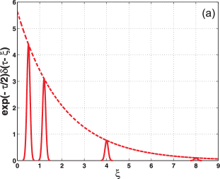
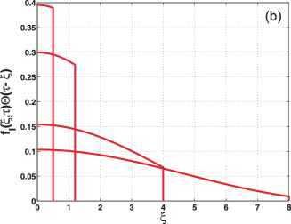
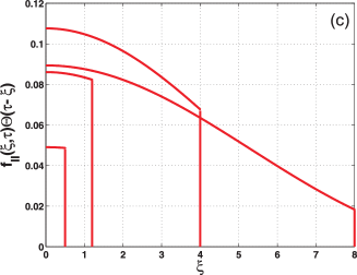
Figure 1: (Color online) The three contributions to the solution of the telegraph equation PDF [equation (11)] for different time intervals $\tau=$ 0.5, 1, 2, 4, 8. Propagating contribution is shown in panel (a). The delta-function is graphically represented by narrow Gaussians [see equation (8)]. The functions $f_{I,II}(\xi,\tau)\Theta(\tau-\xi)$ [see equations (13) and (14)] are shown in panels (b) and (c).

For an arbitrary value of $t_{\mathrm{c}}$, the solution of the telegraph equation is given by three contributions (see, e.g., [15] and the references cited therein)

$$f(\xi,\tau) = \mathrm{e}^{-{\tau}/{2}}\delta(\tau-\xi)+\left[f_{I}(\xi,\tau)+f_{II}(\xi,\tau)\right]\Theta(\tau-\xi)\,.$$ (11)

Here, the two dimensionless variables are the normalized time $\tau=t/t_{\mathrm{c}}$ and the normalized length $\xi=r/\sqrt{Dt_{\mathrm{c}}}$. $\Theta(x)$ is the Heaviside function. The variance of this distribution reads

$$\langle\xi^{2}\rangle_{t}=2\left[\tau-(1-\mathrm{e}^{-\tau})\right].$$ (12)

This form clearly crosses over from ballistic to normal diffusion as $\tau$ increases. The interpretation of the three contributions is as follows: the first term corresponds to the damped ballistic propagation of the kind defined by equation (10). The next two terms exist only inside the compact region that expands with the velocity $c$. The functions $f_{I}(\xi,\tau)$ and $f_{II}(\xi,\tau)$ are given by

$$f_{I}(\xi,\tau)=\frac{\exp(-\tau/2)}{2}I_{0}\bigg{(}\frac{1}{2}\sqrt{\tau^{2}-\xi^{2}}\bigg{)}$$ (13)

and

$$f_{II}(\xi,\tau)=\tau\frac{\exp(-\tau/2)}{2}\frac{I_{1}\bigg{(}\frac{1}{2}\sqrt{\tau^{2}-\xi^{2}}\bigg{)}}{\sqrt{\tau^{2}-\xi^{2}}}\,,$$ (14)

where $I_{\nu}(z)$ are the modified Bessel functions of the first kind. The asymptotic behavior of these functions is defined by $I_{\nu}(z)_{z\to\infty}\sim\exp(z)/\sqrt{2\pi z}$, therefore, in the long time limit $\tau\gg 1$, equation (11) is reduced to the solution of the classical diffusion equation given by equation (4).

Various terms in the solution of the telegraph equation, equation (11), are shown in figure 1. Physically, the first term describes the part of the initial mass of diffusers at the origin that shoots out as a propagating solution which decreases exponentially in time, thus providing more and more mass to the diffusive part of the transport process. The function $f_{I}(\xi,\tau)\Theta(\tau-\xi)$ represents the spreading of diffusers whose mass peaks at the origin without participating in the propagation of the first function. Note that this solution is zero at $t=0$, but it is finite for any positive time. The third term $f_{II}(\xi,\tau)\Theta(\tau-\xi)$ is seen to first increase in weight and in amplitude and later on to decrease. It stems from the existence of a finitely rapid front that does not allow the unphysical infinite speed of propagation that characterizes the solution (4). Of course, the sum of the three contributions is normalized.

3 From the telegraph equation to the time-nonlocal Fokker-Planck
equation

In order to motivate the use of the Fokker-Planck equation with time non-local kernels, we rederive the telegraph equation in the following way: let us begin with the continuity equation in the following form:

$$\frac{\partial f(r,t)}{\partial t}=-\frac{\partial{\bf\Gamma}(r,t)}{\partial r}\,.$$ (15)

Here, ${\bf\Gamma}(r,t)$ is the particle flux. In its turn, this flux satisfies the equation [12]

$$\frac{\partial{\bf\Gamma}(r,t)}{\partial t}=-\frac{{\bf\Gamma}(r,t)-{\bf\Gamma}_{0}(r,t)}{t_{\mathrm{c}}}\,,$$ (16)

where ${\bf\Gamma}_{0}(r,t)$ is the same as the first Fick’s law

$${\bf\Gamma}_{0}(r,t)=-D\frac{\partial f(r,t)}{\partial x}\,.$$ (17)

The solution of equation (16) is given by [17, 18]

$${\bf\Gamma}=-\frac{D}{t_{\mathrm{c}}}\int\limits_{0}^{t}\exp\left(-\frac{t-t^{\prime}}{t_{\mathrm{c}}}\right)\frac{\partial^{2}f(r,t^{\prime})}{\partial r^{2}}\mathrm{d}t^{\prime}.$$ (18)

Substitution of this equation into equation (15) yields the time nonlocal diffusion integro-differential equation

$$\frac{\partial f(r,t)}{\partial t}=\frac{D}{t_{\mathrm{c}}}\int\limits_{0}^{t}\exp\left(-\frac{t-t^{\prime}}{t_{\mathrm{c}}}\right)\frac{\partial^{2}f(r,t^{\prime})}{\partial r^{2}}\mathrm{d}t^{\prime}.$$ (19)

After time differentiation, this equation is reduced to the telegraph equation defined by equation (7).

Observe now [15] that equation (19) is a particular case of the time-nonlocal Fokker-Planck equation,

$$\frac{\partial f(r,t)}{\partial t}=\int_{0}^{t}W(t-t^{\prime})\frac{\partial^{2}f(r,t^{\prime})}{\partial r^{2}}\mathrm{d}t^{\prime}\ ,$$ (20)

where $W(t)$ is the kernel responsible for the non-Fickian behavior of the diffusion process. The Laplace transform of the solution of this equation is given by [19]

$$\widetilde{f}(r,s)=\frac{1}{\widetilde{W}(s)}\cdot\widetilde{P}\left(r,{s}/{\widetilde{W}(s)}\right),$$ (21)

where the function $\widetilde{P}(r,s)$ is the Laplace transform of the solution of the auxiliary equation with the same initial condition

$$\frac{\partial}{\partial t}P(r,t)=\frac{\partial^{2}}{\partial r^{2}}P(r,t)\,.$$ (22)

which is identical with equation (2). The Laplace transform of the solution corresponding to the initial condition defined by equation (3) follows from equation (4) with $D=1$

$$\widetilde{P}(r,s)=\sqrt{\frac{2}{\pi}}\frac{rK_{1/2}\left(r\sqrt{s}\right)}{\left(r\sqrt{s}\right)^{1/2}},$$ (23)

where $K_{1/2}(z)$ is the modified Bessel function of the third kind. Substitution of equation (23) into equation (21) yields the solution of equation (20)

$$\widetilde{f}(r,s)=\sqrt{\frac{2}{\pi}}\frac{r}{\widetilde{W}(s)}\frac{K_{1/2}\left(r\sqrt{s/\widetilde{W}(s)}\right)}{\left(r\sqrt{s/\widetilde{W}(s)}\right)^{1/2}}\,.$$ (24)

The Laplace transform of an even moment of the distribution is defined by

$$\langle r^{2m}\rangle_{s}=\int\limits_{0}^{\infty}\widetilde{f}(x,s)x^{2m}\mathrm{d}x,\qquad m=1,2,\ldots\,.$$ (25)

Substitution of equation (24) into equation (25) yields

$$\langle r^{2m}\rangle_{s}=2m\Gamma(2m)\frac{\widetilde{W}(s)^{m}}{s^{m+1}}\,.$$ (26)

For the moment of zero order, it is necessary to take into account that $\lim_{m\to 0}m\Gamma(2m)=1/2$, therefore, $\langle r^{0}\rangle_{s}=1/s$, i.e., the normalization condition.

For the variance ($m=1$), equation (26) reads

$$\langle r^{2}\rangle_{s}=2\frac{\widetilde{W}(s)}{s^{2}}\,.$$ (27)

The kernel of the time-nonlocal Fokker-Planck equation is defined by the mean square displacement and, therefore, [see equation (20)] the PDF is also defined by this quantity.

4 Determining the kernel from the Langevin equation

The conclusion of the last section is that in order to obtain the appropriate Fokker-Planck equation for a given process, we need to determine the time dependence of the variance $\langle r^{2}\rangle_{t}$. One way to do so is to measure this moment from experimental data. On the other hand, if this data are not available, or if one wants to derive this information from the physics of the problem, another starting point can be the generalized Langevin equation [6, 7].

The standard Langevin equation is Newton’s second law applied to a Brownian particle where the random force acting on a particle is taken into account. As was shown in [20, 21, 22], the generalized Langevin equation is written in terms of a time non-local friction force:

$$\frac{\partial^{2}r(t)}{\partial t^{2}}=-\int\limits_{0}^{t}\gamma(t-t^{\prime})\frac{\partial r(t^{\prime})}{\partial t^{\prime}}\mathrm{d}t^{\prime}+R(t),$$ (28)

where $R(t)$ is the random force component which is uncorrelated with the velocity that has a zero mean $\langle R(t)\rangle=0$. The autocorrelation of the random force is related to the kernel in equation (28) by the fluctuation-dissipation theorem [21, 22]:

$$\langle R(t)R(t^{\prime})\rangle=\frac{k_{\mathrm{B}}T}{m}\gamma(t-t^{\prime}),$$ (29)

where $m$ is the mass of a particle. For the kernel of the kind $\gamma(t)=\gamma_{0}\delta(t)$, equation (28) is transformed to the standard Langevin equation. In the general case, the Fourier transform of the random force correlation function is colored, for example cf. [23]).

In dimensionless variables defined in the section 2 with the diffusion coefficient defined by $D=k_{\mathrm{B}}Tt_{\mathrm{c}}/m$ and $1/t_{\mathrm{c}}=\int_{0}^{\infty}\gamma(t)\mathrm{d}t$, the Laplace transform of the mean square displacement follows from equation (28) (see, e.g., [24]) and reads

$${\widetilde{\langle\xi^{2}\rangle}_{s}}=\frac{2}{s^{2}\left[s+\tilde{\gamma}(s)\right]}\,.$$ (30)

where the dimensionless kernel satisfies in the time domain $\int_{0}^{\infty}\gamma(\tau)\mathrm{d}\tau=1$. One can see from this equation that if $\lim_{s\to\infty}\tilde{\gamma}(s)/s\to 0$, the function $\widetilde{\langle\xi^{2}\rangle}_{s}\sim 1/s^{3}$ and the mean square displacement exhibit the ballistic behavior at short times $\widetilde{\langle\xi^{2}\rangle}_{t}\sim t^{2}$. The shape of the function $\tilde{\gamma}(s)$ at small $s$ is responsible for asymptotic behavior of the mean square displacement in the time domain.

Substitution of equation (30) into equation (27) yields the kernel

$$\widetilde{W}(s)=\frac{1}{s+\tilde{\gamma}(s)}\,.$$ (31)

This equation settles the relation between the memory kernel of the time-nonlocal Fokker-Planck equation and the memory kernel of the Langevin equation.

The solution of equation (20) given by equation (24) with the memory kernel defined by equation (31) reads

$$\widetilde{f}(\xi,s)=\sqrt{\frac{2}{\pi}}\xi\left[s+\tilde{\gamma}(s)\right]\frac{K_{1/2}\left(\xi\sqrt{s\left[s+\tilde{\gamma}(s)\right]}\right)}{\left\{\xi\sqrt{s\left[s+\tilde{\gamma}(s)\right]}\right\}^{1/2}}\,.$$ (32)

Equation (32) consists of two terms,

$$\widetilde{f}(\xi,s)=\xi\left[s+\tilde{\gamma}(s)\right]\widetilde{\Psi}\left(\xi^{2}s\left[s+\tilde{\gamma}(s)\right]\right),$$ (33)

where

$$\widetilde{\Psi}(z)=\sqrt{\frac{2}{\pi}}\frac{K_{1/2}\left(\sqrt{z}\right)}{\left(\sqrt{z}\right)^{1/2}}.$$ (34)

The Taylor expansion of equation (34) is defined by

$$\widetilde{\Psi}(z)=\sum\limits_{n=0}^{\infty}\frac{1}{n!}\frac{\partial^{n}}{\partial z^{n}}\widetilde{\Psi}(z)\Bigg{|}_{z=z_{0}}(z-z_{0})^{n}\,.$$ (35)

For the modified Bessel function of the third kind

$$\frac{\partial^{n}}{\partial z^{n}}\frac{K_{1/2}\left(\sqrt{z}\right)}{\left(\sqrt{z}\right)^{1/2}}=\frac{(-1)^{n}}{2^{n}}\frac{K_{1/2+n}\left(\sqrt{z}\right)}{\left(\sqrt{z}\right)^{1/2+n}}\,.$$ (36)

Equation (33) defines that $z=\xi^{2}s\left[s+\tilde{\gamma}(s)\right]=z_{0}^{2}-\xi^{2}\left[\tilde{\gamma}(s)/2\right]^{2}$, where $z_{0}=\xi^{2}\left\{s+\left[\tilde{\gamma}(s)/2\right]\right\}^{2}$, therefore, equation (35) reads

$$\widetilde{\Psi}(z)=\sqrt{\frac{2}{\pi}}\sum\limits_{n=0}^{\infty}\frac{1}{n!}\frac{K_{1/2+n}\left(\xi\left[s+\tilde{\gamma}(s)/2\right]\right)}{\left\{\xi\left[s+\tilde{\gamma}(s)/2\right]\right\}^{1/2+n}}\left[\frac{\xi\tilde{\gamma}(s)}{2\sqrt{2}}\right]^{2n}\,.$$ (37)

It is suitable to rewrite equation (33) in the following form

$$\widetilde{f}(\xi,s) = r\left\{\left[s+\tilde{\gamma}(s)/2\right]+\tilde{\gamma}(s)/2\right\}\widetilde{\Psi}\left(r^{2}s\left[s+\tilde{\gamma}(s)\right]\right)$$ (38)

$$= \widetilde{f}_{I}(\xi,s)+\widetilde{f}_{II}(\xi,s)\,.$$

Taking into account that

$$K_{1/2}(z)=\sqrt{\frac{\pi}{2}}\frac{\mathrm{e}^{-z}}{\sqrt{z}}$$ (39)

equation (37) can be written as

$$\widetilde{\Psi}(z)=\frac{\exp\left\{-\xi\left[s+\tilde{\gamma}(s)/2\right]\right\}}{\xi\left[s+\tilde{\gamma}(s)/2\right]}+\sum\limits_{n=1}^{\infty}\frac{1}{n!}\frac{K_{1/2+n}\left(\xi\left[s+\tilde{\gamma}(s)/2\right]\right)}{\left\{\xi\left[s+\tilde{\gamma}(s)/2\right]\right\}^{1/2+n}}\left[\frac{\xi\tilde{\gamma}(s)}{2\sqrt{2}}\right]^{2n}\,.$$ (40)

Let $\lim_{s\to\infty}\tilde{\gamma}(s)=\gamma_{0}$. Under this assumption, the sum in equation (40) asymptotically tends to zero and the function defined by equation (40) reads

$$\widetilde{\Psi}(z)\Bigg{|}_{s\to\infty}\sim\frac{\exp\left[-\xi\left(s+{\gamma}_{0}/2\right)\right]}{\xi\left(s+{\gamma}_{0}/2\right)}$$ (41)

and the function $\widetilde{f}_{II}(\xi,s)$ from equation (38) is given by

$$\widetilde{f}_{II}(\xi,s)\Bigg{|}_{s\to\infty}\sim\gamma_{0}\frac{\exp\left[-\xi\left(s+{\gamma}_{0}/2\right)\right]}{s+{\gamma}_{0}/2}\,.$$ (42)

The inverse Laplace transform of equation (42) yields

$${f}_{II}(\xi,t)=\gamma_{0}\mathrm{e}^{-{\gamma_{0}}\tau/{2}}\Theta(\tau-\xi).$$ (43)

proceeding to limit $\lim_{\tau\to 0}{f}_{II}(\xi,\tau)=0$ shows that this contribution to the PDF has nothing to do with the initial condition and is responsible for diffusion of injecting particles during the transport process.

The nonvanishing term in the function $\widetilde{f}_{I}(\tau,s)$ in the limit of large $s$ is defined by

$$\widetilde{f}_{I}(\xi,s)\Bigg{|}_{s\to\infty}\sim\exp\left[-\xi\left(s+{\gamma}_{0}/2\right)\right].$$ (44)

Its inverse Laplace transform yields

$${f}_{I}(\xi,t)=\mathrm{e}^{-{\gamma_{0}}\tau/{2}}\delta(\tau-\xi).$$ (45)

Therefore, the part of the PDF under consideration which is responsible for the initial condition and the further impulse propagation is contained in the first summand in equation (38).

Now we can isolate from the PDF defined by equation (32) the part corresponding to the diffusion process of the particles which are lost by the propagating impulse

$$\widetilde{f}_{\mathrm{diff}}(\xi,s) = \widetilde{f}(\xi,s)-\exp\left[-\xi\left(s+{\gamma}_{0}/2\right)\right]$$ (46)

$$= \widetilde{\Phi}(\xi,s)\mathrm{e}^{-\xi s},$$

where the function $\widetilde{\Phi}(r,s)$ is defined by equation (32) and equation (39) and reads

$$\widetilde{\Phi}(\xi,s) = \left[s+\tilde{\gamma}(s)\right]\frac{\exp\left(-\xi\left\{\sqrt{s\left[s+\tilde{\gamma}(s)\right]}-s\right\}\right)}{\sqrt{s\left[s+\tilde{\gamma}(s)\right]}}-\exp\left(-\frac{\xi\gamma_{0}}{2}\right).$$ (47)

The inverse Laplace transform of equation (47) yields the diffusive part of the PDF in the time domain

$${f}_{\mathrm{diff}}(\xi,t)=\Phi(\xi,\tau-\xi)\Theta(\tau-\xi).$$ (48)

The importance of this result is that the explicit Heaviside function takes upon itself the discontinuity in the function $f_{\mathrm{diff}}(\xi,\tau)$. The function $\Phi(\xi,\tau-\xi)$ in the time domain is a continuous function. If it does not have an analytical representation in a closed form, it can be evaluated numerically, for example using the direct integration method [25].

Summing together the results (45) and (48) in the time domain we get a general solution of the non-Markovian problem with a short-time behavior, in the form

$$f(\xi,\tau) = \mathrm{e}^{-{\gamma_{0}}\tau/{2}}\delta(\tau-\xi)+\Phi(\xi,\tau-\xi)\Theta(\tau-\xi).$$ (49)

From this solution one can see that the diffusion repartition of the PDF occurs inside the spatial diffusion domain which increases in a deterministic way. The first term in equation (49) corresponds to the propagating delta-function which is inherited from the initial conditions, and it keeps decreasing in time at the edge of the ballistically expanding domain.

In order to estimate the PDF in the long time limit, it is necessary to suggest the form of the memory kernel of the Langevin equation at small $s$. The reasonable choice is given by

$$\widetilde{\gamma}(s)_{s\sim 0}\sim s^{\alpha-1}.$$ (50)

One can see from equation (30) that under condition $s^{\alpha+1}\geqslant s^{3}$ (i.e., $\alpha\leqslant 2$) the inverse Laplace transform of equation (30) yields the variance in the form of equation (6). Substitution of equation (50) to equation (32) defines the Laplace transform of the PDF at small $s$

$$\widetilde{f}(\xi,s)=\frac{\exp\left(-\xi s^{\alpha/2}\right)}{s^{1-\alpha/2}}\,.$$ (51)

In the general case, the inverse Laplace transform of equation (51) is given by the Fox functions (see, e.g. [26]). For $\alpha=1$ in the time domain, the PDF is defined by equation (4). For the special case $\alpha=0$, the inverse Laplace transform of equation (51) is independent of time and reads

$$f(\xi)=\mathrm{e}^{-\xi}.$$ (52)

This result coincides with the PDF from [27].

Below we demonstrate the application of the time-nonlocal approach with explicit examples.

4.1 Standard asymptotic diffusion

For $\widetilde{\gamma}(s)=1$ in equation (31) the generalized Langevin equation is reduced to the standard one which predicts the mean square displacement in the form of equation (12). The memory kernel of the time-nonlocal Fokker-Planck equation reads

$$\widetilde{W}(s)=\frac{1}{s+1}\,.$$ (53)

In this case, equation (46) reads

$$\widetilde{f}_{\mathrm{diff}}(\xi,s)=\widetilde{\Phi}(\xi,u)\mathrm{e}^{-\xi u},$$ (54)

where $u=s+1/2$, therefore, the inverse Laplace transform is given by

$$f_{\mathrm{diff}}(\xi,t)=\mathrm{e}^{-\frac{1}{2}t}\Phi(\xi,t-\xi)\Theta(t-\xi).$$ (55)

The function $\widetilde{\Phi}(\xi,u)$ for the particular case under consideration follows from the definition given by equation (47)

$$\widetilde{\Phi}(\xi,u)=u\Psi(\xi,u)-1+\frac{1}{2}\Psi(\xi,u),$$ (56)

where

$$\widetilde{\Psi}(\xi,u)=\frac{\exp\left[-\mid\xi\mid\left(\sqrt{u^{2}-1/4}-u\right)\right]}{\sqrt{u^{2}-1/4}}\,.$$ (57)

From the initial value theorem, it follows that

$$\Psi(\xi,t=0) = \lim_{u\to\infty}u\widetilde{\Psi}(\xi,u)$$ (58)

$$= \lim_{u\to\infty}\frac{\exp\left\{-\mid\xi\mid\left[u\sqrt{1-1/(4u^{2})}-u\right]\right\}}{\sqrt{1-1/(4u^{2})}}=1,$$

Therefore, the inverse Laplace transform of equation (56) is given by

$$\Phi(\xi,t)=\frac{\partial}{\partial t}\Psi(\xi,t)+\frac{1}{2}\Psi(\xi,t).$$ (59)

The inverse Laplace transform of equation (57) is given by [28]

$$\Psi(\xi,t)=I_{0}\left(\frac{1}{2}\sqrt{t^{2}+2\xi t}\right),$$ (60)

where $I_{0}(z)$ is the modified Bessel function.

Substitution of equation (60) into equation (59) yields

$$\Phi(\xi,t)=\frac{1}{2}\left[I_{0}\left(\frac{1}{2}\sqrt{t^{2}+2\xi t}\right)+(t+\xi)\frac{I_{1}\left(\frac{1}{2}\sqrt{t^{2}+2\xi t}\right)}{\sqrt{t^{2}+2\xi t}}\right].$$ (61)

Substitution of this equation into equation (49) reduces the solution to the result for the telegraph equation given by equation (11).

         

Figure 2: (Color online) The diffusion part of the PDF defined by equation (11) for time intervals $\tau=$0.5, 1, 2, 4, 8.

Figure 3: (Color online) The time dependence of the kurtosis of the PDF corresponding to the memory kernel defined by equation (53).

The diffusion part of this solution [the sum of graphics shown in panels (b) and (c) in figure 1] is displayed in figure 3. As was discussed above in the long time limit, this part approaches the solution of the classical diffusion problem given by equation (2). In order to measure how fast the convergence takes place, it is convenient to estimate the time dependence of the kurtosis of the distribution defined by

$$\kappa=\frac{\langle\xi^{4}\rangle}{\langle\xi^{2}\rangle^{2}}-3\,.$$ (62)

For the Gauss distribution $\kappa=0$, for the pure ballistic propagation $\kappa=-2$, moments are defined by equation (26) and for the kernel from equation (53) the second moment is given by equation (12). Calculation of the fourth moment yields

$$\langle\xi^{4}\rangle_{\tau}=12\left[\tau^{2}+6\left(1-\mathrm{e}^{-\tau}\right)-2\tau\left(3+\mathrm{e}^{-\tau}\right)\right].$$ (63)

The kurtosis calculated with these moments is shown in figure 3. At short times, the propagation is ballistic with the following transition to the standard diffusion during a large time interval.

4.2 Anomalous diffusion

In order to join the short time ballistic and long time anomalous regimes [see equation (6) and equation (50)], the Laplace transform of the memory kernel of the Langevin equation can be defined by

$$\widetilde{\gamma}(s)=(2-\alpha)\frac{s^{\alpha-1}}{(1+s)^{\alpha-1}}\,.$$ (64)

It follows from this equation that

$$\gamma_{0}=2-\alpha$$ (65)

and, therefore, the singular part of the PDF is given by

$$f_{I}(\xi,t)=\frac{1}{2}\exp\left[-\frac{3(2-\alpha)}{2}\tau\right]\delta(\mid\xi\mid-\tau)\;.$$ (66)

The diffusion part of the PDF was estimated numerically and is presented in figure 4. The corresponding kurtosis is shown in figure 5.

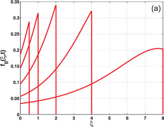
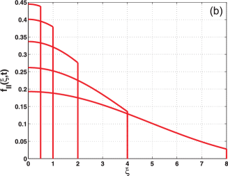
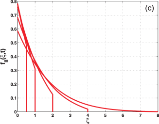
Figure 4: (Color online) The diffusion part of the PDF defined by the memory kernel of the Langevin equation [see equation (64)] for different values of the parameter $\alpha$. Superdiffusion [$\alpha=3/2$, panel (a)], regular diffusion [$\alpha=1$, panel (b)] and subdiffusion [$\alpha=1/2$, panel (c)]. Time intervals from the top to the bottom $\tau=$0.5, 1, 2, 4, 8.

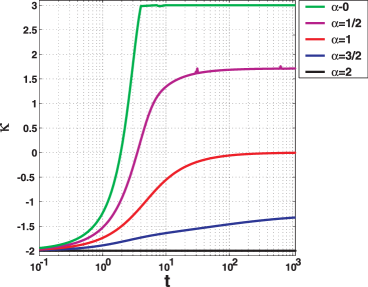
Figure 5: (Color online) The time dependence of the kurtosis of the PDF corresponding to the memory kernel defined by equation (64).

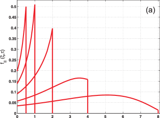
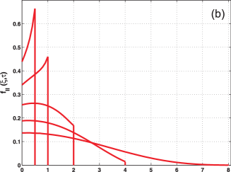
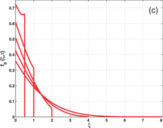
Figure 6: (Color online) The diffusion part of the PDF corresponding to the mean square displacement given by equation (67) for different values of the parameter $\alpha$. Superdiffusion [$\alpha=3/2$, panel (a)], regular diffusion [$\alpha=1$, panel (b)] and subdiffusion [$\alpha=1/2$, panel (c)]. Time intervals from the top to the bottom $\tau=$0.5, 1, 2, 4, 8.

In a different way, the kernel of the time-nonlocal Fokker-Planck equation can be defined by the mean square displacement given in the time domain. In [14] this quantity was proposed in a form interpolating the short time ballistic and long time anomalous behavior

$$\langle\Delta r^{2}\rangle_{t}=2D_{\alpha}t_{0}^{\alpha}\frac{(t/t_{0})^{2}}{\left[1+(t/t_{0})\right]^{2-\alpha}}\,,$$ (67)

where $0\leqslant\alpha\leqslant 2$ and $t_{0}$ is the crossover characteristic time, at $t\ll t_{0}$, the law (67) describes the ballistic regime and at $t\gg t_{0}$ the fractional diffusion.

Introduce now dimensionless variables $\langle\xi^{2}\rangle_{\tau}=\langle\Delta r^{2}\rangle_{t}/(2D_{\alpha}t_{0}^{\alpha})$ and $\tau=t/t_{0}$. With these variables, the last equation reads

$$\langle\xi^{2}\rangle_{\tau}=\frac{\tau^{2}}{(1+\tau)^{2-\alpha}}\,.$$ (68)

The Laplace transform of equation (68) is given by

$$\widetilde{\langle\xi^{2}\rangle}_{s}=\left(\frac{\alpha}{s}-1\right)\frac{1}{s}+\left[(\alpha-1)\left(\frac{\alpha}{s}-2\right)+s\right]\frac{\mathrm{e}^{s}}{s^{\alpha}}\Gamma(\alpha-1,s)\;,$$ (69)

where $\Gamma(a,s)$ is the incomplete gamma function. At large $s$ equation can be written as

$$s^{2}\frac{\widetilde{\langle\xi^{2}\rangle}_{s}}{k_{B}T}\Bigg{|}_{s\to\infty}\sim\frac{2}{s}-\frac{2\gamma_{0}}{s^{2}}+\ldots\,.$$ (70)

Substitution of equation (69) into equation (70) yields the estimation of the asymptotic value of the memory kernel $\gamma_{0}=3(2-\alpha)$ which defines the time evolution of the singular part of the PDF. The results of numerical calculations of the diffusive part are shown in figure 6

The time evolution of the kurtosises of these distributions is displayed in figure (7).

The reader should appreciate the tremendous role of memory. The ballistic part which is represented by the advancing and reducing delta-function sends backwards the probability that it loses due to the exponential decay seen in figure 1, panel (a). Thus, the diffusive part of the PDF is replenished with time and asymptotically approaches the Markovian distribution. The speed of convergence and the evolution of the PDF shape depends on the interim behavior of the mean square displacement (or, which is the same, of the memory kernel of the Langevin equation).

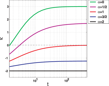
Figure 7: (Color online) The time dependence of the kurtosis of the PDF corresponding to the mean square displacement defined by equation (67).

5 Hydrodynamic theory of the time-nonlocal diffusion

5.1 Memory kernel

The friction force acting upon a spherical particle has been derived in [29, 30] (the modern discussion can be found in [31]) and is given by

$$F_{\mathrm{fr}}(t)=-2\pi R^{3}\left[\frac{3\eta}{R^{2}}u(t)+\frac{\rho}{3}\frac{\partial u(t)}{\partial t}+\frac{3}{R}\sqrt{\frac{\rho\eta}{\pi}}\int\limits_{0}^{t}\frac{1}{\sqrt{t-\tau}}\frac{\partial u(\tau)}{\partial\tau}\mathrm{d}\tau\right],$$ (71)

where $F_{\mathrm{fr}}(t)$ is the friction force, $R$ is the particle radius, and $\rho$ and $\eta$ are the density and viscosity of the solvent. Substitution of this force into the Langevin equation yields the fractional equation, and the Laplace transform of the memory kernel can be found in a straightforward way [32]. For simplicity instead of this approach we will use the results obtained [16] for the mean square displacement.

A system with hydrodynamic memory has two characteristic times

$$\tau_{R}=\frac{9}{2}\frac{M_{\mathrm{s}}}{S}\,,$$ (72)

where $M_{\mathrm{s}}$ is the mass of a solvent particle, $S=6\pi\eta R$ is the Stokes friction coefficient and

$$\tau_{\mathrm{F}}=\frac{M+M_{\mathrm{s}}/2}{S}=\frac{1}{9}\Bigg{(}1+2\frac{M}{M_{\mathrm{s}}}\Bigg{)}\tau_{R}\,.$$ (73)

One can see from equation (73) that $\tau_{\mathrm{F}}>0$. Therefore, it is reasonable to introduce dimensionless variables $\tau=t/\tau_{\mathrm{F}}$ and $\beta=\tau_{R}/\tau_{\mathrm{F}}$. Then, the projection of the mean square displacement onto one of the axis reads

$$\langle\Delta x^{2}(\tau)\rangle = 2D\tau_{\mathrm{F}}\Bigg{\{}\tau-2\left({{\beta}\tau/{\pi}}\right)^{1/2}+(\beta-1)$$ (74)

$$+\frac{1}{\alpha_{1}-\alpha_{2}}\Bigg{[}\frac{1}{\alpha_{1}^{3}}\mathrm{e}^{\alpha_{1}^{2}\tau}\mathrm{erfc}\left(\alpha_{1}\sqrt{\tau}\right)-\frac{1}{\alpha_{2}^{3}}\mathrm{e}^{\alpha_{2}^{2}\tau}\mathrm{erfc}\left(\alpha_{2}\sqrt{\tau}\right)\Bigg{]}\Bigg{\}}\;,$$

where $D$ is the diffusion coefficient, $\mathrm{erfc}(z)$ is the complimentary error function and coefficients $\alpha_{1}$ and $\alpha_{2}$ are given by

$$\alpha_{1,2}=\frac{1}{2}\Bigg{(}\sqrt{\beta}\mp\sqrt{\beta-4}\Bigg{)}.$$ (75)

The dependence of the coefficients $\alpha_{1}$ and $\alpha_{2}$ on the parameter $\beta$ is shown in figure 9.

Figure 8: (Color online) Dependence of coefficients $\alpha_{1,2}$ on the parameter $\beta$.

Figure 9: (Color online) Time dependence of the mean square displacement for different values of the parameter $\beta$ [$\langle\xi(\tau)^{2}\rangle=\langle x^{2}(\tau)\rangle/(2D\tau_{\mathrm{F}})$].

At short times $\tau\ll 1$, the mean square displacement is given by the Taylor expansion of equation (74)

$$\langle\Delta x^{2}(\tau)\rangle = 2D\tau_{\mathrm{F}}\tau^{2}\Bigg{\{}\frac{1}{2}-\frac{8}{15}\left({{\beta\tau}/{\pi}}\right)^{1/2}+\frac{1}{6}(\beta-1)\tau$$ (76)

$$+\frac{16}{105}\left({{\beta\tau}/{\pi}}\right)^{1/2}\tau+\frac{1}{24}\left[\beta(\beta-3)+1\right]\tau^{2}+\cdots\Bigg{\}}.$$

One can see that the mean square displacement defined by equation (76) corresponds to the ballistic motion.

In the long time limit, the mean square displacement is given by

$$\langle\Delta x^{2}(\tau)\rangle=2D\tau_{\mathrm{F}}\tau\left\{1-2\left({{\beta}/{\pi\tau}}\right)^{1/2}+\frac{\beta-1}{\tau}-\left({{\beta}/{\pi}}\right)^{1/2}\left[\frac{\beta-2}{\sqrt{\tau}\tau}-\frac{(\beta-1)(\beta-3)}{2\sqrt{\tau}\tau^{3}}\right]\right\}.$$ (77)

equation (77) agrees with the standard diffusive.

On can see in figure (9) that there are a few particular points.

1. $\beta=0$, ($M_{\mathrm{s}}=0$). Substitution of this value of the parameter $\beta$ into equation (75) yields $\alpha_{1,2}=\pm\mathrm{i}$ and equation (74) is reduced to equation (12).

2. $\beta=3$ ($M=M_{\mathrm{s}}$). In this case, $\alpha_{1,2}=(\sqrt{(}3)\mp\mathrm{i})/2$ and the mean square displacement is defined by the error function of complex argument.

3. $\beta=4$ ($M/M_{\mathrm{s}}=5/8$). Substitution of $\beta=4$ into equation (75) yields $\alpha_{1(2)}=1$. It follows from equation (74) that

   $$\lim_{\alpha_{1}\to\alpha_{2}=1}\langle x^{2}(\tau)\rangle=2D\tau_{\mathrm{F}}\left[\tau-6\sqrt{\frac{\tau}{\pi}}+3+(2\tau-3)\mathrm{e}^{\tau}\mathrm{erfc}\left(\sqrt{\tau}\right)\right].$$ (78)

4. $\beta=9$ ($M=0$). In this case, the real parameters $\alpha_{1,2}=(3\mp\sqrt{5})/2$.

The mean square displacements for different values of the parameter $\beta$ listed above are shown in figure 9. The hydrodynamic interaction results in time delay of the mean square displacement. The larger is the value of the parameter $\beta$, the slower is the convergence to the asymptotic limit.

It is necessary to note that the predictions of equation (74) are in a good agreement with experimental data [9]

The Laplace transform of the mean square displacement given by equation (74) reads

$$\langle\widetilde{\Delta\xi^{2}(s)}\rangle=\frac{2}{s^{2}\left(s+1+\sqrt{\beta s}\right)}\,,$$ (79)

therefore, the memory kernel of the Langevin equation is given by

$$\widetilde{\gamma}(s)=1+\sqrt{\beta s}\,.$$ (80)

Substitution of equation (80) to equation (31) yields the kernel of the time-nonlocal Fokker-Planck equation with due regard for hydrodynamics effects

$$\widetilde{W}(s)=\frac{1}{s+1+\sqrt{\beta s}}\,.$$ (81)

5.2 Probability density function

Solutions of the telegraph equation in higher than one dimension were considered in [33] and it was shown that the result is unphysical, in some regions the PDF becomes negative. Nevertheless, a reasonable PDF in explicit form was obtained for two-dimensional systems within the framework of a persistent random walk model [34]. Therefore, the possibility to describe the high dimension diffusion process with finite speed of propagation using the time-nonlocal approach is an open question.

In the general case, equation (20) reads in dimensionless units

$$\frac{\partial f(\xi,\tau)}{\partial\tau}=\int_{0}^{\tau}W(\tau-\tau^{\prime})\Delta_{d}f(\xi,\tau^{\prime})\mathrm{d}\tau^{\prime}\ ,$$ (82)

where $d$ is the space dimension and the Laplace operator is given by

$$\Delta_{d}=\frac{1}{\xi^{d-1}}\frac{\partial}{\partial\xi}\xi^{d-1}\frac{\partial}{\partial\xi}=\frac{\partial^{2}}{\partial\xi^{2}}+\frac{d-1}{\xi}\frac{\partial}{\partial\xi}\,.$$ (83)

For pure ballistic propagation, the kernel in equation (82) is defined by $W(\tau)\equiv 1$. The time derivative of equation (82) with this kernel yields d-dimensional wave equation

$$\frac{\partial^{2}f(\xi,\tau)}{\partial\tau^{2}}-\Delta_{d}f(\xi,\tau)=0.$$ (84)

It is clear that the propagation of the ballistic impulse is specified by the function

$$f(\xi,\tau)=\frac{\delta(\tau-\xi)}{\xi^{d-1}}\,,$$ (85)

where the normalization condition is defined by $\int_{0}^{\infty}f(\xi,\tau)\xi^{d-1}\mathrm{d}\xi=1$. Nevertheless, this function is the solution of equation (84), i.e., the one-dimensional case only; for higher dimensions, the solution differs from the function defined by equation (85), turning negative in some regions. This is the source of the failure of the telegraph equation for $d>1$. Substitution of equation (85) into equation (84) yields

$$\bigg{(}\frac{\partial^{2}}{\partial\tau^{2}}-\Delta_{d}\bigg{)}\frac{\delta(\tau-\xi)}{r^{d-1}}=\frac{d-1}{\xi}\Bigg{(}\frac{\partial}{\partial\xi}+\frac{d-2}{\xi}\Big{)}\frac{\delta(\tau-\xi)}{\xi^{d-1}}\,.$$ (86)

Therefore, we can suggest that the auxiliary equation which corresponds to equation (86) should be given by

$$\frac{\partial f(\xi,\tau)}{\partial\tau}=\frac{\partial^{2}f(\xi,\tau)}{\partial\xi^{2}}+2\frac{d-1}{\xi}\frac{\partial f(\xi,\tau)}{\partial\xi}+\frac{(d-1)(d-2)}{\xi^{2}}f(\xi,\tau).$$ (87)

The Laplace transform of equation (87) reads

$$\frac{\partial^{2}\widetilde{f}(\xi,s)}{\partial\xi^{2}}+2\frac{d-1}{\xi}\frac{\partial\widetilde{f}(\xi,s)}{\partial\xi}+\left[\frac{(d-1)(d-2)}{\xi^{2}}-s\right]\widetilde{f}(\xi,s)=0.$$ (88)

This equation can be reduced to the Bessel equation [35] and its normalized solution is given by

$$\widetilde{f}(\xi,s)=\sqrt{\frac{2}{\pi}}\xi^{2-d}\frac{K_{1/2}\left(\xi\sqrt{s}\right)}{\left(\xi\sqrt{s}\right)^{1/2}}\,.$$ (89)

The inverse Laplace transform of equation (89) yields the PDF in the time domain

$$f(\xi,\tau)=\frac{1}{\sqrt{\pi}}\xi^{1-d}\frac{\mathrm{e}^{-\xi^{2}/(4\tau)}}{\sqrt{\tau}}\,.$$ (90)

The PDF given by this equation differs from that of standard diffusion. Nevertheless, the second moment of this function is in agreement with equation (1) and the kurtosis of this distribution is given by $\kappa=3$.

We suggest that the time-nonlocal Fokker-Planck equation should be given by

$$\frac{\partial f(\xi,\tau)}{\partial\tau}=\int_{0}^{\tau}W(\tau-\tau^{\prime})\hat{\mathcal{D}}f(\xi,\tau^{\prime})\mathrm{d}\tau^{\prime},$$ (91)

where the operator $\hat{\mathcal{D}}$ is defined by

$$\hat{\mathcal{D}}=\frac{\partial^{2}}{\partial\xi^{2}}+2\frac{d-1}{\xi}\frac{\partial}{\partial\xi}+\frac{(d-1)(d-2)}{\xi^{2}}\ .$$ (92)

The formal solution of equation (91) follows from equation (89) and equation (31)

$$\widetilde{f}(\xi,s)=\sqrt{\frac{2}{\pi}}\xi^{2-d}\left[s+\widetilde{\gamma}(s)\right]\frac{K_{1/2}\left(\xi\sqrt{s\left[s+\widetilde{\gamma}(s)\right]}\right)}{\left(\xi\sqrt{s\left[s+\widetilde{\gamma}(s)\right]}\right)^{1/2}}\,.$$ (93)

This equation is similar to equation (32) to within the coefficient which depends on $\xi$. Therefore, the nonvanishing part of the PDF for $d=3$ and the memory kernel defined by equation (80) is given [see equation (40) and equation (44)] by

$$\widetilde{f}_{I}(\xi,s)=\frac{1}{\xi^{2}}\exp\left[-r\left(s+\frac{1+\sqrt{\beta s}}{2}\right)\right].$$ (94)

For $\beta=0$, the inverse Laplace transform of this equation yields the damped impulse propagation corresponding to equation (85). In a general case, the inverse Laplace transform of equation (94) reads

$${f}_{I}(\xi,\tau)=\frac{1}{4\xi}\mathrm{e}^{-\xi/2}\sqrt{\frac{\beta}{\pi}}\frac{\exp\left\{-\beta\xi^{2}/\left[16(\tau-\xi)\right]\right\}}{\sqrt{(\tau-\xi)^{3}}}\,.$$ (95)

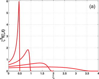
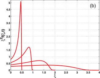
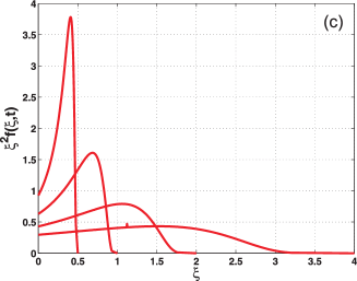
Figure 10: (Color online) The PDF defined by equation (96) for $t=0.5,1,2,4$. Panel (a): $\beta=3$; Panel (b): $\beta=4$; Panel (c): $\beta=9$

In the limit $\tau\to 0$, the function defined by equation (95) tends to three-dimensional delta-function, i.e., the initial condition of the problem under consideration. In infinitesimal time, the delta-function due to hydrodynamic interactions becomes smooth and the PDF is free from the singular contribution. Therefore, there is no need to pull out the ballistic contribution from the full PDF, and the solution of the problem is given by

$$f(\xi,\tau)=\Phi(\xi,\tau-\xi)\Theta(\tau-\xi),$$ (96)

where the inverse Laplace transform of the continuous function is

$$\widetilde{\Phi}(\xi,s) = \left[{1+{1}/{s}+\left({{\beta}/{s}}\right)^{1/2}}\right]^{1/2}\exp\left(-\mid\xi\mid\cdot s\left\{\left[{1+{1}/{s}+\left({{\beta}/{s}}\right)^{1/2}}\right]^{1/2}-1\right\}\right)\,.$$ (97)

This can be estimated numerically. The results of calculations for different values of the parameter $\beta$ are shown in figure 10. Note that a similar ballistic peak of the PDF was observed in simulations of the test particle transported in pseudoturbulent fields [36]. The kurtosis of the PDF for different values of the parameter $\beta$ are compared in figure 11.

6 Conclusion

The strategy followed in this paper is to construct a time-nonlocal Fokker-Planck equation which reproduces the time dependence of the mean square displacement of an underlying process throughout the time domain. It should be stressed that the same mean square displacement may correspond, in general, to different models for the time-dependence of the PDF. Thus, the predictions of the time non-local Fokker-Planck approach should be compared to experimental data for the PDF to assess its scope of validity and the quality of the approximation. The advantage of the proposed model is that it can deal with diffusion processes that cross-over from a ballistic to a fractional behavior when time increases from short to long values, respectively.

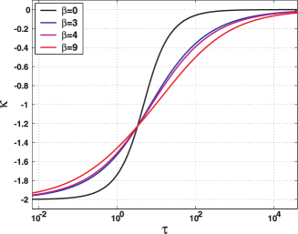
Figure 11: (Color online) The time dependence of the kurtosis of the PDF corresponding to the memory kernel defined by equation (81).

The general one-dimensional solution (49) demonstrates the effect of the temporal memory in the form of a partition of the probability distribution function inside a growing spatial domain which increases in a deterministic way. The approach provides a solution that exists at all times, and, in particular, is free from the instantaneous action puzzle. An extension of the employed approach to higher spatial dimensions is used to study the implications of hydrodynamic interactions on the shape of the PDF. It is shown that singular ballistic contribution to the PDF is smoothed out during the propagation. The expansion given by equation (37) splits the Laplace transform of the PDF into two parts. One part is the ballistic part which is the solution of an inhomogeneous differential equation in spatial variable with the initial condition of the problem. The second one is the diffusion part, which solved the homogeneous equation and is zero at the initial time. In its turn, the diffusion part is divided again into a few terms which correspond, in general, to different auxiliary equations. Therefore, each diffusion term in $s$-space can be multiplied by a coefficient $C(s)$ so that the normalization condition and the mean square displacement are preserved. Moreover, there is a freedom of modelling here, and this freedom has not been exhausted in this paper. Further analysis and comparison with experimental systems are necessary to nail down the various options of modeling different physical realizations. This research will be the subject of the coming publications.

Ukrainian 0

Рiвняння Фокера-Планка з пам’яттю: кросовер вiд балiстичного до дифузiйного процесу в багаточастинкових системах i нестисних середовищах

В. Iльїн${}^{\textsf{\footnotesize{\mbox{?}}}}$, I. Прокаччiа${}^{\textsf{\footnotesize{\mbox{?}}}}$, A. Загороднiй${}^{\textsf{\footnotesize{\mbox{?}}}}$

             
${}^{\textsf{\footnotesize 1}}$ Вiддiл хiмiчної фiзики, Науковий Iнститут Вайцмана, 76100 Реховот, Iзраїль ${}^{\textsf{\footnotesize 2}}$ Iнститут теоретичної фiзики iм. М.М. Боголюбова НАН України, 03680 Київ, Україна

References

- [1] Philibert J., Diffusion Fundamentals, 2005, 2, 1.
- [2] Hurst H.E., Trans. Am. Soc. Civil Eng., 1951, 116, 770.
- [3] Mandelbrot B.B., van Ness J.W., SIAM Rev., 1968, 10, 422; doi:10.1137/1010093.
- [4] Einstein A., Ann. Phys., 1905, 17, 549.
- [5] Einstein A., Ann. Phys., 1906, 19, 371.
- [6] Langevin P., C. R. Acad. Sci. (Paris), 1908, 146, 530.
- [7] Lemons D.S., Gythiel A., Am. J. Phys., 1997, 65, 1079; doi:10.1119/1.18725.
- [8] Uhlenback G.E., Ornstein L.S., Phys. Rev., 1930, 36, 823¦ doi:10.1103/PhysRev.36.823.
-
[9]
Lukić B., Jeney S., Tischer C., Kulik A.J., Forró L.,
Florin E.L., Phys. Rev. Lett., 2005, 95, 160601;
doi:10.1103/PhysRevLett.95.160601. -
[10]
Huang R., Chavez I., Taute K.M., Lukić B., Jeney S.,
Raizen M.G., Florin E.L., Nat. Phys., 2011, 7,
576;
doi:10.1038/nphys1953. - [11] Pusey P.N., Science, 2011, 332, 802; doi:10.1126/science.1192222.
- [12] Davydov B.I., Dokl. Akad. Nauk SSSR, 1934, 2, 474.
- [13] Morse P.M., Feshbach H., Methods of Theoretical Physics, McGraw-Hill, New York, 1953.
- [14] Ilyin V., Procaccia I., Zagorodny A., Phys. Rev. E, 2010, 81, 030105(R); doi:10.1103/PhysRevE.81.030105.
- [15] Ilyin V., Zagorodny A., Ukr. J. Phys., 2010, 55, 235.
- [16] Vladimirsky V., Terletzky Y.A., Zh. Eksp. Teor. Fiz., 1945, 15, 258 (in Russian).
- [17] Cattaneo C., Atti. Sem. Mat. Fis. Univ. Modena, 1948, 3, 83.
-
[18]
Reverberia A.P., Bagnerini P., Maga L., Bruzzone A.G., Int. J. Heat Mass Transfer, 2008, 51, 5327;
doi:10.1016/j.ijheatmasstransfer.2008.01.039. - [19] Sokolov I.M., Phys. Rev. E, 2002, 66, 041101; doi:10.1103/PhysRevE.66.041101.
- [20] H. Mori, Prog. Theor. Phys., 1965, 33, 423; doi:10.1143/PTP.33.423.
- [21] R. Kubo, The Fluctuation-Dissipation Theorem and Brownian Motion, 1965 Tokyo Summer Lectures in Theoretical Physics, Part 1. Many-Body Theory, Kubo R. (Ed.), Syokabo, Tokyo and Benjamin, New York, 1966, 1–16.
- [22] Kubo R., Rep. Prog. Phys., 1966, 29, 255; doi:10.1088/0034-4885/29/1/306.
- [23] Luczka J., Chaos, 2005, 15, 026107; doi:10.1063/1.1860471.
- [24] Porrà J.M., Wang K.-G., Masoliver J., Phys. Rev. E, 1996, 53, 5872; doi:10.1103/PhysRevE.53.5872.
- [25] Duffy D.G., ACM TOMS, 1993, 19, 333; doi:10.1145/155743.155788.
- [26] Metzler R., Klafter J., Phys. Rep., 2000, 339, 1; doi:10.1016/S0370-1573(00)00070-3.
- [27] Ball R.C., Havlin S., Weiss G.H., J. Phys. A: Math. Gen., 1987, 20, 4055; doi:10.1088/0305-4470/20/12/052.
- [28] Handbook of Mathematical Functions with Formulas, Graphs, and Mathematical Tables, Abramowitz M., Stegun I.A. (Eds.), Dover, New York, 1972.
- [29] Boussinesq J.V., C. R. Acad. Sci., 1885, 100, 935.
- [30] Basset A.B., Treatise on Hydrodynamics., Vol. 2, Dover, New York, 1961, Chap.22.
- [31] Landau L.D., Lifshitz E.M., Fluid Mechanics, Pergamon Press, Oxford, New York, 1987.
- [32] Mainardi F., Pironi P., Extr. Math., 1996, 11, 140.
- [33] Porrà J.M., Masoliver J., Weiss G.H., Phys. Rev. E, 1997, 55, 7771; doi:10.1103/PhysRevE.55.7771.
- [34] Masoliver J., Porrà J.M., Weiss G.H., Physica A, 1993, 193, 469; doi:10.1016/0378-4371(93)90488-P.
- [35] Kamke E., Differentialgleichungen. Lösungsmethoden und Lösungen I. Gewöhnliche Differentialgleichungen, Leipzig, 1942.
- [36] Hauff T., Jenko F., Eule S., Phys. Plasmas, 2007, 14, 102316; doi:10.1063/1.2794322.
Ukrainian \adddialect\l@ukrainian0 \l@ukrainian