Probing CMB Secondary Anisotropies through Minkowski Functionals

Abstract

Secondary contributions to the anisotropy of the Cosmic Microwave Background (CMB), such as the integrated Sachs-Wolfe (ISW) effect, the thermal Sunyaev-Zel’dovich effect (tSZ), and the effect of gravitational lensing, have distinctive non-Gaussian signatures, and full descriptions therefore require information beyond that contained in their power spectra. The Minkowski Functionals (MF) are well-known as tools for quantifying any departure from Gaussianity and are affected by noise and other sources of confusion in a different way from the usual methods based on higher-order moments or polyspectra, thus providing complementary tools for CMB analysis and cross-validation of results. In this paper we use the recently introduced skew-spectra associated with the MFs to probe the topology of CMB maps to probe the secondary non-Gaussianity as a function of beam-smoothing in order to separate various contributions. We devise estimators for these spectra in the presence of a realistic observational masks and present expressions for their covariance as a function of instrumental noise. Specific results are derived for the mixed ISW-lensing and tSZ-lensing bispectra as well as contamination due to point sources for noise levels that correspond to the Planck ($143$ GHz channel) and EPIC ($150$ GHz channel) experiments. The cumulative signal to noise ration $S/N$ for one-point generalized skewness-parameters can reach an order of ${\cal O}(10)$ for Planck and two orders of magnitude higher for EPIC, i.e. ${\cal O}(10^{3})$. We also find that these three spectra skew-spectra are correlated, having correlation coefficients $r\sim 0.5-1.0$; higher $l$ modes are more strongly correlated. Though the values of $S/N$ increase with decreasing noise, the triplets of skew-spectra that determine the MFs become more correlated; the $S/N$ ratios of lensing-induced skew-spectra are smaller compared to that of a frequency-cleaned tSZ map.

1 Introduction

All-sky multi-frequency Cosmic Microwave Background (CMB) missions, such as the completed WMAP, ongoing Planck and future (proposed) Experimental Probe of Inflationary Cosmology (EPIC) survey (Bock et al., 2008, 2009; Baumann et al., 2009) or ESAs Cosmic Origin Explorer (COrE, The COrE Collaboration (2012)) are major sources of information about the properties of the primordial density fluctuations that seeded the process of galaxy formation in the Universe as well as other key aspects of cosmological theory, including the global isotropy (Copi et al., 2007; Hoftuft et al., 2009; Hanson & Lewis, 2009) and topology of the Universe (Luminet et al., 2003; Roukemia et al., 2004).

The study of non-Gaussianity in the CMB fluctuations can provide valuable and detailed information regarding the physics of the early Universe of the inflationary epoch In the standard slow-roll paradigm, the scalar field responsible for inflation fluctuates with a minimal amount of self interaction which ensures that any non-Gaussianity generated during the inflation through self-interaction is expected to be small (Salopek & Bond, 1990, 1991; Falk et al., 1993; Gangui et al., 1994; Acquaviva et al., 2003; Maldacena, 2003); see Bartolo, Matarrese & Riotto (2006) for a review. Variants of the simple inflationary model such as multiple scalar fields, features in the inflationary potential, non-adiabatic fluctuations, non-standard kinetic terms, warm inflation, or deviations from Bunch-Davies vacuum can however all lead to higher level of primordial non-Gaussianity (Chen, 2010).

However, the detection of departure from Gaussianity in the CMB can be due to either primary or secondary effects (or both), as well as the mode-coupling effects of secondaries and gravitational lensing along the observer’s light cone. Secondary anisotropies resulting from the formation of structure are known to dominate at smaller angular scales, are highly non-Gaussian in nature (Cooray, 2001b; Cooray & Hu, 2000; Verde & Spergel, 2002) and are arguably as interesting as their primary counterpart. One of the prominent contributions to the secondary non-Gaussianity is due to the mode-coupling of weak gravitational lensing and sources of secondary contributions such as the thermal Sunyaev-Zel’dovich effect (Goldberg & Spergel, 1999a, b; Cooray & Hu, 2000). Although weak lensing of the CMB produces its own characteristic signature in the angular power spectrum, its detection has proved to be difficult using the CMB power spectrum alone. Non-Gaussianity imprinted by lensing into the primordial CMB remains below the detection level of current experiments, although with Planck the situation is likely to improve. Nevertheless, cross-correlating CMB data with external tracers means lensing signals can be probed at the level of the mixed bispectrum. After the first unsuccessful attempt to cross-correlate WMAP against SDSS, recent efforts by Smith, Zahn & Dore (2007) have found a clear signal of weak lensing of the CMB, by cross-correlating WMAP against NVSS. Their work also underlines the link between three-point statistical estimators and the estimators for weak lensing effects on CMB. The understanding of secondaries are not only important in their own right, but also from the perspective of their impact on estimation of cosmological parameters (Smidt, 2010).

The study of non-Gaussianity is usually primarily focused on the bispectrum, as this saturates the Cramér-Rao bound (Babich, 2005; Kamionkowski, Smith & Heavens., 2011) and is therefore in a sense optimal, however in practice it is difficult to probe the entire configuration dependence in harmonic space contained within the bispectrum using noisy data (Munshi & Heavens, 2010). The cumulant correlators are multi-point correlators collapsed to encode two-point statistics. These were introduced in the context of analyzing galaxy clustering by Szapudi & Szalay (1999), and were later found to be useful for analyzing projected surveys such as the APM galaxy survey(Munshi, Melott & Coles, 2000). Being two-point statistics they can be analyzed in multipole space by defining an associated power-spectrum. Recent studies by Cooray (2006) and Cooray, Li & Melchiorri (2008) have demonstrated their wider applicability including, e.g., in 21cm studies. In more recent studies the skew- and kurt-spectra were found to be useful for analysing temperature (Munshi & Heavens, 2010) as well as polarization maps (Munshi et al., 2011c) from CMB experiments and in weak lensing studies (Munshi et al., 2011b, d).

In addition to studies involving lower order multi-spectra, MFs have been extensively developed as a statistical tool for non-Gaussianity in a cosmological setting for both 2-dimensional (projected) and 3-dimensional (redshift) surveys. Analytic results are known certain properties of the MFs of a Gaussian random field making them suitable for identifying non-Gaussianity. Examples of such studies include CMB data (Schmalzing & Górski, 1998; Novikov, Schmalzing and Mukhanov, 2000; Hikage et al., 2008; Natoli et al., 2010), weak lensing (Matsubara and Jain (2001); Sato et al. (2001); Taruya et al. (2002); Munshi et al. (2012a)), large-scale structure (Gott et al., 1986; Coles, 1988; Gott et al., 1989; Melott, 1990; Gott et al., 1990; Moore et al., 1992; Gott et al., 1992; Canavezes et al., 1998; Sahni, Sathyaprakash & Shandarin, 1998; Schmalzing & Diaferio, 2000; Kerscher et al., 2001; Hikage et al., 2002; Park et al., 2005; Hikage, Komatsu & Mastubara, 2006; Hikage et al., 2008), 21cm (Gleser et al., 2006), frequency cleaned Sunyaev-Zel’dovich (SZ) maps (Munshi et al., 2012b) and N-body simulations (Schmalzing & Diaferio, 2000; Kerscher et al., 2001). The MFs are spatially-defined topological statistics and, by definition, contain statistical information of all orders in the moments. This makes them complementary to the poly-spectra methods that are defined in Fourier space. It is also possible that the two approaches will be sensitive to different aspects of non-Gaussianity and systematic effects although in the weakly non-Gaussian limit it has been shown that the MFs reduce to a weighted probe of the bispectrum (Hikage, Komatsu & Mastubara (2006)).

The skew-spectrum is a weighted statistic that can be tuned to a particular form of non-Gaussianity, such as that which may arise either during inflation at an early stage or from structure formation at a later time. The skew-spectrum retains more information about the specific form of non-Gaussianity than the (one-point) skewness parameter alone. This allows not only the exploration of primary and secondary non-Gaussianity but also the residuals from galactic foreground and unresolved point sources. The skew-spectrum is directly related to the lowest order cumulant correlator and is also known as the two-to-one spectra in the literature (Cooray, 2001a). In a series of recent publications the concept of skew-spectra was generalized to analyse the morphological properties of cosmological data sets or in particular the MFs by Munshi, Smidt & Cooray (2010); Munshi et al. (2012a, b); Pratten & Munshi (2012). The first of these three spectra, in the context of secondary-lensing correlation studies, was introduced by Munshi et al. (2011a) and was subsequently used to analyse data release from WMAP by Calabrese et al. (2010).

The primary aim of this paper is to consider the entire set of generalised skew-spectra resulting from the mode-coupling of secondary anisotropies and lensing of the CMB and the contribution thereof to non-Gaussian morphology of the CMB maps. We will be considering three different secondary-lensing correlation bispectra. The secondaries that we consider are the Integrated Sachs-Wolfe effect (ISW) that dominates at large angular scales (Cooray, 2002) and the thermal Sunyaev-Zel’dovich (tSZ) effect that dominates at smaller angular scales Birkinshaw (1999). In addition we consider a foreground, namely the contribution from unresolved point sources. We will consider two experimental setups, the ongoing Planck satellite and the the proposed EPIC satellite mission discussed above.

The layout of the paper is as follows. In §2 we briefly outline the bispectrum corresponding to lensing-secondary mode-coupling. Next, in §3, we review the formalism underlying the Minkowski Functionals and in §4 we introduce the generalised skew-spectra associated with the MFs. In §5 we present the estimators for these spectra and their covariances. Finally, in §7 we discuss our results and comment on future implementation.

Throughout we will use the parameters of a WMAP cosmology (Larson et al., 2011).

2 Mode Coupling induced by Lensing - Secondary Cross-correlation and the resulting Bispectrum

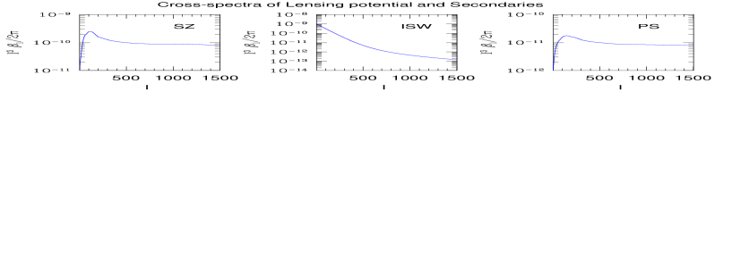
Figure 1: The cross-spectra $\beta_{l}$ for various secondaries and lensing are plotted as a function of the harmonics $l$. From left to right different panels correspond to cross-correlation of lensing potential and SZ, ISW and PS contribution. The cross-spectra $\beta_{l}$ is being used in Eq.(10) for the construction of mixed bispectrum $B^{\rm PLS}_{l_{1}l_{2}l_{3}}$. It is defined in Eq.(14). Various estimators for the skew-spectra that we will use, associated with the three MFs, will be defined using the mixed bispectra. A background $\Lambda$CDM cosmology is assumed. The details of these calculations, which relies on halo model prescriptions, can be found in (Cooray, 2001a).

The bispectrum of primary anistropies encodes information that can be used to constrain the inflationary dynamics but, as discussed in the previous section, the primary contribution to non-Gaussianity is expected to be negligible in the simplest realisations of the generic inflationary scenario.

The secondary bispectrum provides valuable information regarding the low-redshift Universe and constrains structure formation scenarios. The secondaries can be broadly divided into three different types:

1. Gravitational secondaries, caused by evolution in the gravitational potential along the observer’s past light cone including the well-known integrated Sachs-Wolfe (ISW) effect (Kofman & Starobinsky, 1985; Martinez-Gonzaléz, Sanz, Silk, 1990; Mukhanov, Feldman & Bandenberger, 1992; Kaminkowski & Spergel, 1994; Munshi, Souradeep & Starobinsky, 1995; Mollerach et al., 1995; Boughn & Crittenden, 2004) as well as the Rees-Sciama (RS) effect.

2. Scattering secondaries, such as the thermal Sunyaev-Zel’dovich (tSZ) effect (Birkinshaw, 1999), kinetic Sunyaev Zel’dovich (kSZ) effect and the Ostriker-Vishniac effect (see e.g. Castro et al. (2004)). These effects are caused by the interaction of the CMB photons with the intervening free-electron population.

3. Lensing secondaries caused by the propagation of photons through large scale structures.

Contributions to secondary bispectra can also arise from terms involving the cross-correlation of gravitational lensing and the effects of intervening material, such as the tSZ effect due to inverse Compton scattering of CMB photons from hot gas in the intervening clusters. The decay of the peculiar gravitational potential along the line of sight in $\Lambda$CDM cosmology, introduced above as the Integrated Sachs-Wolfe or ISW effect, is correlated to the lensing due to the potential, can also generate an additional contribution to the secondary bispectrum in a similar fashion; see e.g. Cooray & Seth (2002) for a detailed discussion of various secondaries in the context of halo model. The contribution to secondaries due to reionization of the Universe are detailed in Hu, Scott & Silk (1994). Foregrounds, such as unresolved point sources (PS), can also contribute to the secondary bispectrum through their cross-correlation with the lensing of CMB.

On a different note, we comment that while the study of secondary anisotropies is important in their own right, they are also important in their effect on the calculation of error covariances in cosmological parameter estimation (Joudaki et al., 2010). Understanding the detailed statistical properties of secondary anisotropies like those we discuss here is therefore is of the utmost importance in the era of precision cosmology.

We will be dealing with the secondary bispectra involving the lensing of both primary anistropies and other secondaries. Following Goldberg & Spergel (1999a), Goldberg & Spergel (1999b) and Cooray & Hu (2000) we start by expanding the observed temperature anisotropy in terms of the primary contribution $\Theta_{\rm P}({\hat{\Omega}})$, the secondary contribution $\Theta_{\rm S}({\hat{\Omega}})$ and lensing of the primary $\Theta_{\rm L}({\hat{\Omega}})$:

$$\Theta({\hat{\Omega}})=\Theta_{\rm P}({\hat{\Omega}})+\Theta_{\rm L}({\hat{\Omega}})+\Theta_{\rm S}({\hat{\Omega}})+\cdots.$$ (1)

Here ${\hat{\Omega}}=(\theta,\phi)$ is the angular position on the surface of the sky. Expanding the respective contribution in terms of spherical harmonics $Y_{lm}({\hat{\Omega}})$ we can write:

$$\Theta_{\mathrm{P}}({\hat{\Omega}})\equiv\sum_{lm}(\Theta_{\rm p})_{lm}Y_{lm}({\hat{\Omega}});~{}~{}~{}~{}\Theta_{\mathrm{L}}({\hat{\Omega}})\equiv\sum_{lm}[\nabla\psi({\hat{\Omega}})\cdot\nabla\Theta_{\mathrm{P}}({\hat{\Omega}})]_{lm}\;Y_{lm}({\hat{\Omega}});~{}~{}~{}~{}\Theta_{\mathrm{S}}({\hat{\Omega}})\equiv\sum_{lm}(\Theta_{\rm S})_{lm}Y_{lm}({\hat{\Omega}}).$$ (2)

Here $\psi({\hat{\Omega}})$ is the projected lensing potential (Goldberg & Spergel, 1999a, b). The secondary bispectrum for the CMB takes contributions from products of P, L and S terms with varying order. The bispectrum $B_{l_{1}l_{2}l_{3}}^{\rm PLS}$ are defined as follows (see Bartolo et al. (2004) for generic discussion on the bispectrum and its symmetry properties):

$$B_{l_{1}l_{2}l_{3}}^{\rm PLS} \equiv\sum_{m_{1}m_{2}m_{3}}\left(\begin{array}[]{ c c c }l_{1}&l_{2}&l_{3}\\ m_{1}&m_{2}&m_{3}\end{array}\right)\int\left\langle\Theta_{\rm P}({\hat{\Omega}}_{1})\Theta_{\rm L}({\hat{\Omega}}_{2})\Theta_{\rm S}({\hat{\Omega}}_{3})\right\rangle Y^{*}_{l_{1}m_{1}}({\hat{\Omega}}_{1})Y^{*}_{l_{2}m_{2}}({\hat{\Omega}}_{2})Y^{*}_{l_{3}m_{3}}({\hat{\Omega}}_{3})d{\hat{\Omega}}_{1}d{\hat{\Omega}}_{2}d{\hat{\Omega}}_{3};$$ (8)

$$\equiv\sum_{m_{1}m_{2}m_{3}}\left(\begin{array}[]{ c c c }l_{1}&l_{2}&l_{3}\\ m_{1}&m_{2}&m_{3}\end{array}\right)\langle(\Theta_{\mathrm{\rm P}})_{l_{1}m_{1}}(\Theta_{\mathrm{\rm L}})_{l_{2}m_{2}}(\Theta_{\mathrm{\rm S}})_{l_{3}m_{3}}\rangle.$$

The angular brackets represent ensemble averages. The matrices denote $3j$ symbols (Edmonds, 1968) and the asterisks denote complex conjugation. It is possible to invert the relation assuming isotropy of the background Universe:

$$\langle(\Theta_{\mathrm{P}})_{l_{1}m_{1}}(\Theta_{\mathrm{L}})_{l_{2}m_{2}}(\Theta_{\mathrm{S}})_{l_{3}m_{3}}\rangle=\left(\begin{array}[]{ c c c }l_{1}&l_{2}&l_{3}\\ m_{1}&m_{2}&m_{3}\end{array}\right)B^{\rm PLS}_{l_{1}l_{2}l_{3}}.$$ (9)

Finally the bispectrum $B_{l_{1}l_{2}l_{3}}^{\rm PLS}$ is expressed in terms of the un-lensed primary power spectrum ${\cal C}_{l}=\langle(\Theta_{\rm P})_{lm}(\Theta_{\rm P}^{*})_{lm}\rangle$ and the cross-spectra $\beta_{l}$ (to be defined below) as follows:

$$B_{l_{1}l_{2}l_{3}}^{\rm PLS}=-\left\{\beta_{l_{3}}{\cal C}_{l_{1}}{l_{2}(l_{2}+1)-l_{1}(l_{1}+1)-l_{3}(l_{3}+1)\over 2}+{\rm cyc.perm.}\right\}I_{l_{1}l_{2}l_{3}}\equiv{\cal B}_{l_{1}l_{2}l_{3}}I_{l_{1}l_{2}l_{3}};$$ (10)

$$I_{l_{1}l_{2}l_{3}}\equiv\sqrt{(2l_{1}+1)(2l_{2}+1)(2l_{3}+1)\over 4\pi}\left(\begin{array}[]{ c c c }l_{1}&l_{2}&l_{3}\\ 0&0&0\end{array}\right).$$ (13)

(see Goldberg & Spergel (1999a), Goldberg & Spergel (1999b) for a derivation). The reduced bispectrum above is denoted ${\cal B}_{l_{1}l_{2}l_{3}}$. To simplify the notation for the rest of this paper, we henceforth drop the superscript $\rm PLS$ form the bispectrum $B_{l_{1}l_{2}l_{3}}$. The cross-spectrum $\beta_{l}$ introduced above represents the cross-correlation between the projected lensing potential $\psi({\hat{\Omega}})$ and the secondary contribution $\Theta_{\rm S}({\hat{\Omega}})$:

$$\langle\psi({\hat{\Omega}})\Theta_{\rm S}({\hat{\Omega}}^{\prime})\rangle={1\over 4\pi}\sum_{l=2}^{l_{\rm max}}(2l+1)\beta_{l}P_{l}(\hat{\Omega}\cdot\hat{\Omega}^{\prime}).$$ (14)

The cross-spectra $\beta_{l}$ take different forms for ISW-lensing, RS-lensing or SZ-lensing correlation and we assume a zero primordial non-Gaussianity. The reduced bispectrum ${\cal B}_{l_{1}l_{2}l_{3}}$ defined above using the notation $I_{l_{1}l_{2}l_{3}}$ is useful in separating the angular dependence from the dependence on power spectra $C_{l}$ and $\beta_{l}$. We will use this to express the topological properties of the CMB maps. The $\beta_{l}$ parameters for lensing secondary correlations are displayed in Figure-1. The left, middle and right panels in Figure-1 displays SZ-lensing, ISW-lensing and point source lensing correlations. These results are based on halo model calculations performed using the halo model (Cooray, 2001a).

The beam $b_{l}(\theta_{b})$ and the noise of a specific experiment are characterised by the parameters $\sigma_{\rm beam}$ and $\sigma_{\rm rms}$:

$$b_{l}(\theta_{b})=\exp[-l(l+1)\sigma_{\rm beam}^{2}];\;\;\;\sigma_{\rm beam}={\theta_{b}\over\sqrt{8\ln(2)}};\;\;\;n_{l}=\sigma_{\rm rms}^{2}\Omega_{\rm pix};\quad\Omega_{\rm pix}={4\pi\over{\rm N}_{\rm pix}}.$$ (15)

where $\sigma_{\rm rms}$ is the rms noise per pixel that depends on the full width at half maxima or FWHM of the beam $\theta_{b}$. The number of pixel ${\rm N}_{\rm pix}$ required to cover the sky determines the size of the pixels $\Omega_{\rm pix}$. To incorporate the effect of experimental noise and the beam we have to replace ${\cal C}_{l}\rightarrow{\cal C}_{l}b_{l}^{2}(\theta_{b})+n_{l}$, and the normalization of the skew-spectra that we will introduce later will be affected by the experimental beam and noise. The computation of scatter will also depend on these parameters. We will consider two different experimental setups: Planck and EPIC. The parameters of these experiments are tabulated in Table 1.

The optimal estimators for lensing-secondary mode-coupling bispectrum have been recently discussed by Munshi et al. (2011a). The estimators that we propose here are relevant in the context of constructing the MFs.

3 Minkowski functionals

Integral geometry provides a natural framework within which to define the set of morphological descriptors for a random field. These descriptors are intrinsically defined in the spatial domain where they take into account all $n$-point correlators up to arbitrary order. Hadwiger’s characterization theorem shows that a linear combination of these $d+1$ functionals will provide a complete morphological description of the morphology of $d$-dimensional objects; see Hadwiger (1959) for a formal treatment. These functionals are more commonly referred to as the Minkowski functionals. The Minkowski Functionals are usually calculated using volume-weighted curvature integrals for which the analytical results for a Gaussian random field are known (Adler, 1981; Tomita, 1986; Gott et al., 1990). More recently the analytical values for weakly non-Gaussian fields have been calculated as a function of skewness parameters by using a perturbative approach based on the Edgeworth expansion (Matsubara, 1994, 1995; Matsubara & Yokohama, 1996; Matsubara, 2002; Hikage, Komatsu & Mastubara, 2006)). This approach allows us to use the MFs as a test of non-Gaussianity in the weakly perturbed regime as constrained by observation and predicted by models for inflation.

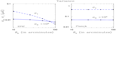
Figure 2: The variances $\sigma_{0}(\theta_{b})$ and $\sigma_{1}(\theta_{b})$, defined in Eq.(19), are plotted as a function of the FWHM $\theta_{b}$. The left panel corresponds to an experimental setup such as EPIC and the right panel corresponds to Planck-type experiment.See Table-1 for detail specifications regarding the noise level and beam.

In 2 dimensions the MFs $V_{0}(\nu)$, $V_{1}(\nu)$ and $V_{2}(\nu)$ correspond respectively to the area of a set $\Sigma$, length of the perimeter of the set and the integrated curvature along its boundary. The MF $V_{2}(\nu)$ can be related to the well-known genus $g$ and the Euler characteristic $\chi$:

$$V_{0}(\nu)=\int_{\Sigma}da;\quad V_{1}(\nu)={1\over 4}\int_{\partial\Sigma}dl;\quad V_{2}(\nu)={1\over 2\pi}\int_{\partial\Sigma}\kappa dl.$$ (16)

Here $dl$ and $da$ represent the length and surface element respectively. In our analysis we consider a smoothed random field ${\Theta}({\hat{\Omega}})$ with mean $\langle{\Theta}({\hat{\Omega}})\rangle=0$ and variance $\sigma_{0}^{2}(\theta_{b})=\langle{\Theta}^{2}({\hat{\Omega}})\rangle$. For a generic 2-dimensional weakly non-Gaussian random field ${\Theta}$ on the surface of the sky, the spherical harmonic decomposition using $Y_{lm}({\hat{\Omega}})$ as basis functions ${\Theta}({\hat{\Omega}})=\sum_{lm}{\Theta}_{lm}Y_{lm}({\hat{\Omega}})$ can be used to define the power spectrum ${\cal C}_{l}$ which is sufficient to characterize an isotropic Gaussian field $\langle{\Theta}_{lm}{\Theta}^{*}_{l^{\prime}m^{\prime}}\rangle={\cal C}_{l}\delta_{ll^{\prime}}\delta_{mm^{\prime}}$.

We will be studying the MFs defined over the surface of the celestial sphere but equivalent results can be obtained in 3D using a Fourier decomposition (Pratten & Munshi, 2012). The MFs for a 3D random Gaussian field are well known and are given by Tomita’s formula (Tomita, 1986).

For a non-Gaussian field the higher order statistics such as bi- or tri-spectrum can describe the resulting mode-mode coupling. Alternatively topological measures such as the MFs (including the Euler characteristic or genus) can be employed to quantify deviations from Gaussianity. Indeed it can be shown that the information content in both descriptions is equivalent in that, at leading order, the MFs can be constructed completely from the knowledge of the bispectrum alone.

The notations and analytical results in this section are being kept generic however they will be specialized to the case of CMB sky in subsequent discussions.

The MFs denoted as $V_{k}(\nu)$ for a threshold $\nu={\Theta}/\sigma_{0}$; where $\sigma^{2}_{0}(\theta_{b})=\langle{\Theta}^{2}\rangle$ are perturbatively expressed as:

$$V_{k}(\nu)={1\over(2\pi)^{(k+1)/2}}{\omega_{2}\over\omega_{2-k}\omega_{k}}\exp\left(-{\nu^{2}\over 2}\right)\left(\sigma_{1}\over\sqrt{2}\sigma_{0}\right)^{k}\left[V_{k}^{(2)}(\nu)\sigma_{0}(\theta_{b})+V_{k}^{(3)}(\nu)\sigma_{0}^{2}(\theta_{b})+V_{k}^{(4)}(\nu)\sigma_{0}^{3}(\theta_{b})+\cdots\right]$$ (17)

$$V_{k}^{(2)}(\nu)=\left[\left\{{1\over 6}S^{(0)}(\theta_{b})H_{k+2}(\nu)+{k\over 3}S^{(1)}(\theta_{b})H_{k}(\nu)+{k(k-1)\over 6}S^{(2)}(\theta_{b})H_{k-2}(\nu)\right\}\right]$$ (18)

$$\sigma_{j}^{2}(\theta_{b})={1\over 4\pi}\sum_{l}(2l+1)[l(l+1)]^{j}{\cal C}_{l}b_{l}^{2}(\theta_{b})$$ (19)

The constant $\omega_{k}$ introduced above is the volume of the unit sphere in $k$ dimensions. $w_{k}={\pi^{k/2}/\Gamma(k/2+1)}$ in 2-dimension we will only need $\omega_{0}=1$, $\omega_{1}=2$ and $\omega_{2}=\pi$. Here $\Gamma$ is the the gamma function. The lowest-order Hermite polynomials $H_{k}(\nu)$ are listed below.

$$H_{-1}(\nu)=\sqrt{\pi\over 2}\exp\left({\nu^{2}\over 2}\right){\rm erfc}\left(\nu\over\sqrt{2}\right);\quad H_{0}(\nu)=1,\quad H_{1}(\nu)=\nu,{}$$

$$H_{2}(\nu)=\nu^{2}-1,\quad H_{3}(\nu)=\nu^{3}-3\nu,\quad\quad H_{4}(\nu)=\nu^{4}-6\nu^{2}+3,{}$$

$$H_{n}(\nu)=(-1)^{n}\exp\left({\nu^{2}\over 2}\right){d\over d\nu^{n}}\exp\left(-{\nu^{2}\over 2}\right).$$ (20)

The expression consists of two distinct contributions. The part that does not depend on the three different skewness parameters $S^{(0)}(\theta_{b}),S^{(1)}(\theta_{b}),S^{(2)}(\theta_{b})$ and signifies the MFs for a Gaussian random field. The other contribution $\delta V_{k}(\nu)$ represents the departure from the Gaussian statistics and depends on the generalized skewness parameters defined in Eq.(22) - Eq.(24).

perturbatively

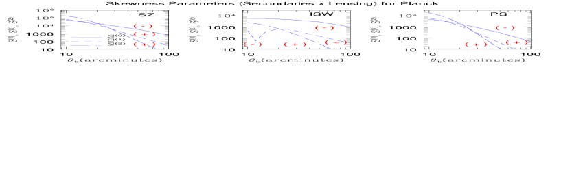
Figure 3: Same as previous plot but for Planck type noise. The normalisation of the skew spectra is depends on the noise level. The shape of the bispectrum is independent of the noise but depends on the experimental beam. Notice that $S^{(1)}(\theta_{b})$ changes sign near $\theta_{b}\sim 10^{\prime}$ as before. $S^{(0)}(\theta_{b})$ is negative for all three effects. The other parameters remain positive for the entire range of FWHM probed.

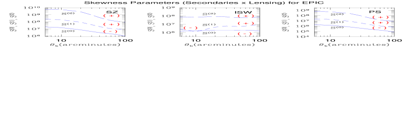
Figure 4: The absolute magnitudes of the one-point skewness parameters $S^{(0)}(\theta_{b})$, $S^{(1)}(\theta_{b})$ and $S^{(2)}(\theta_{b})$ (solid, short-dashed and long dashed lines respectively), are plotted as a function of smoothing scale $\theta_{b}$. These parameters are defined in Eq.(21). Various panels correspond to contributions from different types of secondary non-Gaussianity that represent the cross-correlation of lensing and Sunyaev-Zel’dovich effect (left-panel), cross-correlation of ISW and lensing (middle-panel) and cross-correlation of point sources and lensing (right-panel). The parameter $S^{(0)}(\theta_{b})$ is negative for the entire range of FWHM or $\theta_{b}$ considered, for all three bispectra we have studied. The parameter $S^{(1)}(\theta_{b})$ shows a transition from being negative to positive for the case of ISW bispetcrum. All other skewness parameters stays positive as indicated. An experimental set up which is same as EPIC was considered. See Table-1 for detailed specifications regarding level of noise and beam. The bispectrum used in our calculation is given in Eq.(10) and the cross-spectra are plotted in Figure-1.

Various second-order moments $\sigma_{j}(\theta_{b})$ defined in Eq.(19) appear in Eq.(17) and Eq.(18) can be expressed in terms of the power spectra ${\cal C}_{l}$ and the observational beam $b_{l}(\theta_{b})$, assumed Gaussian with a full width at half maximum $\theta_{b}$; see Eq.(15) for definition. The moment $\sigma_{0}(\theta_{b})$ is a special case which relates to the variance of the field. The quantities $\sigma_{1}(\theta_{b})$, $\sigma_{2}(\theta_{b})$ are natural generalization of this variance, putting greater weight on higher-order harmonics; the variances that appear most frequently henceforth are $\sigma_{0}^{2}(\theta_{b})=\langle{\Theta}^{2}\rangle$ and $\sigma_{1}^{2}(\theta_{b})=\langle(\nabla{\Theta})^{2}\rangle$.

Real space expressions for the triplets of skewness $S^{(i)}(\theta_{b})$ are given below. These are natural generalizations of the ordinary skewness $S^{(0)}(\theta_{b})$ that is used in many cosmological studies. They are all cubic statistics but are constructed from different cubic combinations.

$${S}^{(0)}(\theta_{b})\equiv{S^{({\Theta}^{3})}(\theta_{b})\over\sigma_{0}^{4}(\theta_{b})}={\langle{\Theta}^{3}\rangle\over\sigma_{0}^{4}(\theta_{b})};\quad{S}^{(1)}(\theta_{b})\equiv-{3\over 4}{S^{({\Theta}^{2}\nabla^{2}{\Theta})}(\theta_{b})\over\sigma_{0}^{2}(\theta_{b})\sigma_{1}^{2}(\theta_{b})}=-{3\over 4}{\langle{\Theta}^{2}\nabla^{2}{\Theta}\rangle\over\sigma_{0}^{2}(\theta_{b})\sigma_{1}^{2}(\theta_{b})};\quad{}$$

$$S^{(2)}(\theta_{b})\equiv-3{S^{(\nabla{\Theta}\cdot\nabla{\Theta}\nabla^{2}{\Theta})}(\theta_{b})\over\sigma_{1}^{4}(\theta_{b})}=-{3}{\langle(\nabla{\Theta}).(\nabla{\Theta})(\nabla^{2}{\Theta})\rangle\over\sigma_{1}^{4}(\theta_{b})}.$$ (21)

Notice that a knowledge of the $S^{(i)}(\theta_{b})$ parameters completely specifies the $V_{k}^{(2)}(\nu)$ parameters which characterize the lowest order departure from Gaussianity. The expressions in the harmonic domain are more useful in the context of CMB studies where these skewness parameters can be recovered from a masked sky using analytical tools that are commonly used for power spectrum analysis. The skewness parameter $S^{(1)}(\theta_{b})$ is constructed from the product field $[{\Theta}^{2}]$ and $[\nabla^{2}{\Theta}]$, whereas skewness parameter $S^{(2)}(\theta_{b})$ relies on the combination of $[\nabla{\Theta}\cdot\nabla{\Theta}]$ and $[\nabla^{2}{\Theta}]$. By construction, the skewness parameter $S^{(2)}(\theta_{b})$ has the highest weight for high $l$ modes and $S^{(0)}_{b}$ has the lowest weight from high $l$ modes.

The expressions in terms of the bispectrum $B_{l_{1}l_{2}l_{3}}$ (see Eq.(8) for definition) take the following form:

$$S^{({\Theta}^{3})}(\theta_{b})={1\over 4\pi}\sum_{l_{i}=2}^{l_{max}}B_{l_{1}l_{2}l_{3}}I_{l_{1}l_{2}l_{3}}b_{l_{1}}(\theta_{b})b_{l_{2}}(\theta_{b})b_{l_{3}}(\theta_{b}),$$ (22)

$$S^{({\Theta}^{2}\nabla^{2}{\Theta})}(\theta_{b})=-{1\over 12\pi}\sum_{l_{i}=2}^{l_{max}}{}\Big{[}{l_{1}(l_{1}+1)+l_{2}(l_{2}+1)+l_{3}(l_{3}+1)}\Big{]}B_{l_{1}l_{2}l_{3}}I_{l_{1}l_{2}l_{3}}b_{l_{1}}(\theta_{b})b_{l_{2}}(\theta_{b})b_{l_{3}}(\theta_{b}),$$ (23)

$$S^{(\nabla{\Theta}\cdot\nabla{\Theta}\nabla^{2}{\Theta})}(\theta_{b})={1\over 4\pi}\sum_{l_{i}=2}^{l_{max}}{}\Big{[}[l_{1}(l_{1}+1)+l_{2}(l_{2}+1)-l_{3}(l_{3}+1)]l_{3}(l_{3}+1)+{\rm cyc.perm.}\Big{]}B_{l_{1}l_{2}l_{3}}I_{l_{1}l_{2}l_{3}}b_{l_{1}}(\theta_{b})b_{l_{2}}(\theta_{b})b_{l_{3}}(\theta_{b}).$$ (24)

The dependence of the skew spectra $S^{(i)}(\theta_{b})$ and the beam $b_{l}(\theta_{b})$ on the smoothing angular scale $\theta_{b}$ is being suppressed for brevity.

The angular bispectrum $B_{l_{1}l_{2}l_{3}}$ contains all the information at the level of the three-point angular correlation function. These results are generic and do not assume any specific form of non-Gaussianity. However, to arrive at specific expressions we will ignore the primordial non-Gaussianity, known to be sub-dominant, and concentrate on secondary non-Gaussianity. There is a family of one-point statistics, namely the well-known skewness parameters $S^{(i)}(\theta_{b})$ introduced above, or pseudo-collapsed three-point function (Hinsaw et al., 1995), as well as the equilateral configuration statistics (Ferreira, Magueijo & Gorski, 1998) which can all be expressed as linear combinations of the bispectrum terms. The generalized skewness parameters introduced above are also all linear combinations of the bispectrum weights but with varying weights. Using one-point statistics has the advantage of higher signal to noise but the price we pay is in terms of reduced power to discriminate individual contributions.

The series expansion for the MFs can be extended beyond the leading order at the level of the bispectrum to the next-to-leading order which involves the trispectrum of the temperature field. The lensing induced trispectrum of the CMB will constitute the main next-to-leading order contribution. It is also important to realize that measurements of skewness parameters $S^{(0)}(\theta_{b})$, $S^{(1)}(\theta_{b})$ and $S^{(2)}(\theta_{b})$ will not be independent but correlated with one another; the level of correlation depends on the noise and beam profile.

In Figure 2 we have plotted the variance parameters $\sigma^{2}_{0}(\theta_{b})$ and $\sigma^{2}_{1}(\theta_{b})$ for various smoothing beams (assumed Gaussian). The four different FWHM that are considered are $\theta_{b}=10^{\prime},25^{\prime},50^{\prime}$ and $100^{\prime}$ respectively. The parameter values only depend on the underlying CMB power spectra and the beam as well as the noise. They are used as a normalization parameters while constructing the MFs from the generalized skewness parameters. Two different beam and noise levels are considered EPIC (left-panel) and Planck (right-panel). The one-point generalised skewness parameters are depicted in Figure-3 for Planck and Figure-4 for EPIC. The background cosmology is that of $\Lambda$CDM.

In Figure 4 the one-point skewness parameters $S^{(0)}(\theta_{b})$, $S^{(1)}(\theta_{b})$ and $S^{(2)}(\theta_{b})$ (solid, short-dashed and long dashed lines respectively), are plotted as a function of smoothing scale $\theta_{b}$. These parameters are defined in Eq.(21). The panels correspond to contributions from different types of secondary non-Gaussianity: cross-correlation of lensing and Sunyaev-Zel’dovich effect (left-panel), cross-correlation of ISW and lensing (middle-panel); cross-correlation of point source and lensing (right-panel). An experimental set up which is same as EPIC was considered. See Table 1 for detail specifications regarding level of noise and beam. The bispectrum used in our calculation is given in Eq.(10) and the cross-spectra is plotted in Figure 3 we plot the one-point skewness parameters for Planck.

4 The triplets of Skew-Spectra and Lowest Order Corrections to Gaussian MFs

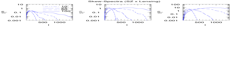
Figure 5: The three skew-spectra corresponding to the three MFs $S_{l}^{(0)}(\theta_{b})$ (left-panel) , $S_{l}^{(1)}(\theta_{b})$ (middel-panel) and $S_{l}^{(2)}(\theta_{b})$ (right-panel) are plotted for the mixed secondary bispectrum of SZ$\times$Lensing as a function of the harmonics $l$. A background $\Lambda$CDM cosmology is assumed.The skew-spectra are defined in Eq(22), Eq(23) and Eq(24) respectively. All other sources of non-Gaussianity are ignored. Four different Gaussian-beams are considered. The curves from left to right correspond to $\theta_{b}=10^{\prime},25^{\prime},50^{\prime},100^{\prime}$ in each panel. The normalization of the skew spectra is somewhat arbitrary and do not affect the signal to noise ratios. We have ignored the presence of noise, as defined in Eq.(19), in our calculation of $\sigma_{0}(\theta_{b})$ and $\sigma_{1}(\theta_{b})$ respectively. Notice that for a given $\theta_{b}$ higher order skew-spectra peak at a higher $l$. The signal to noise of the skew-spectra associated with SZ effect are plotted in Figure 9 for EPIC and Figure 8 for Planck noise level respectively. The skew-spectra are not uncorrelated. The cross-correlation among various skew-spectra are displayed in Figure 11 for EPIC and Figure 10 for Planck.

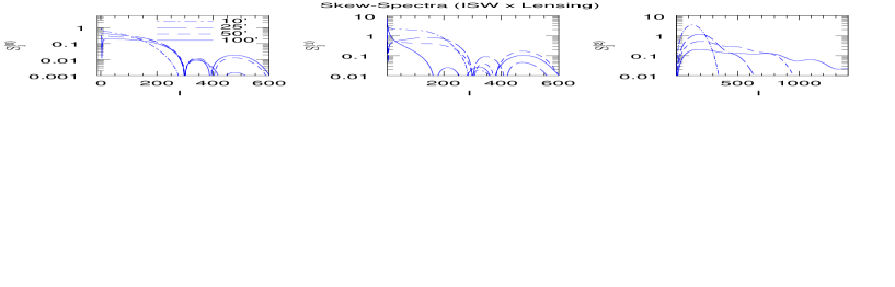
Figure 6: The skew-spectra $S_{l}^{(0)}(\theta_{b})$, $S_{l}^{(1)}(\theta_{b})$ and $S_{l}^{(2)}(\theta_{b})$ for ISW$\times$Lensing is plotted as a function of the harmonics $l$. Notice that skew-spectra corresponding to ISW are dominant at smaller $l$s while the ones corresponding to SZ dominate at larger $l$ values. The skew-spectra, being integrated measures, depend on the entire harmonic range of the bispectra. The shape of the skew-spectra can play an important role in separating individual contributions of secondary non-Gaussianity.

The skew-spectrum has been studied previously in various cosmological contexts (Cooray, 2001a), e.g. to estimate the bispectrum resulting from lensing-SZ correlation. The skew-spectra are cubic statistics constructed by cross-correlating two different fields. One of the fields used is a composite field (map) typically a product of two maps either in its original form or constructed by means of applying relevant differential operators. Example of such derived maps that we will consider are $[\Theta^{2}({\hat{\Omega}})],[\nabla\Theta({\hat{\Omega}})\cdot\nabla\Theta({\hat{\Omega}})]$ and $[\nabla^{2}\Theta({\hat{\Omega}})]$. The skew-spectra resulting from cross-correlating these maps are known as the generalised skew spectra and are related to the three generalised skewness parameters introduced above. At the lowest order, the MFs themselves can be constructed using these generalized skewness parameters and contain equivalent information.

The detection of each individual mode of the primary or secondary bispectrum is still considered challenging. This is primarily due to the low signal-to-noise associated with each individual modes. All available information is therefore typically compressed into a single number - the skewness. This drastic data compression leads to a significant degradation of the power of the statistic to discriminate between models.

The first of the skew-spectra that we will study is the one introduced by (Cooray, 2001a) and later generalized Munshi & Heavens (2010). It is related to sometimes known as the two-to-one power spectrum and is constructed by cross-correlating the squared map $[{\Theta}^{2}({\hat{\Omega}})]$ with the original map ${\Theta}({\hat{\Omega}})$. The second skew-spectrum is constructed by cross-correlating the squared map $[{\Theta}^{2}({\hat{\Omega}})]$ with $[\nabla^{2}{\Theta}({\hat{\Omega}})]$. Analogously the third skew-spectrum represents the cross-spectra that can be constructed using $[\nabla{\Theta}({\hat{\Omega}})\cdot\nabla{\Theta}({\hat{\Omega}})]$ and $[\nabla^{2}{\Theta}({\hat{\Omega}})]$ maps.

$$S_{l}^{(0)}(\theta_{b})\equiv{1\over 12\pi\sigma_{0}^{4}(\theta_{b})}S_{l}^{({\Theta}^{2},{\Theta})}(\theta_{b})\equiv{1\over 12\pi\sigma_{0}^{4}(\theta_{b})}{1\over 2l+1}\sum_{m}{\rm Real}([{\Theta}]_{lm}[{\Theta}^{2}]^{*}_{lm})={1\over 12\pi\sigma_{0}^{4}(\theta_{b})}\sum_{l_{1}l_{2}}B_{ll_{1}l_{2}}J_{ll_{1}l_{2}}b_{l}(\theta_{b})b_{l_{1}}(\theta_{b})b_{l_{2}}(\theta_{b}),$$ (25)

$$S_{l}^{(1)}(\theta_{b})\equiv{1\over 16\pi\sigma_{0}^{2}(\theta_{b})\sigma_{1}^{2}(\theta)}S_{l}^{({\Theta}^{2},\nabla^{2}{\Theta})}(\theta_{b})\equiv{1\over 16\pi\sigma_{0}^{2}(\theta_{b})\sigma_{1}^{2}(\theta_{b})}{1\over 2l+1}\sum_{m}{\rm Real}([\nabla^{2}{\Theta}]_{lm}[{\Theta}^{2}]^{*}_{lm}){}$$

$$\quad\quad={1\over 16\pi\sigma_{0}^{2}(\theta_{b})\sigma_{1}^{2}(\theta_{b})}\sum_{l_{i}}\Big{[}{l(l+1)+l_{1}(l_{1}+1)+l_{2}(l_{2}+1)}\Big{]}B_{ll_{1}l_{2}}J_{ll_{1}l_{2}}b_{l_{1}}(\theta_{b})b_{l_{2}}(\theta_{b})b_{l_{3}}(\theta_{b}),$$ (26)

$$S_{l}^{(2)}(\theta_{b})\equiv{1\over 8\pi\sigma_{1}^{4}(\theta_{b})}S_{l}^{(\nabla{\Theta}\cdot\nabla{\Theta},\nabla^{2}{\Theta})}(\theta_{b})\equiv{1\over 8\pi\sigma_{1}^{4}(\theta_{b})}{1\over 2l+1}\sum_{m}{\rm Real}([\nabla{\Theta}\cdot\nabla{\Theta}]_{lm}[\nabla^{2}{\Theta}]^{*}_{lm}){}$$

$$\quad\quad={1\over 8\pi\sigma_{1}^{4}(\theta_{b})}\sum_{l_{i}}{}\Big{[}[l(l+1)+l_{1}(l_{1}+1)-l_{2}(l_{2}+1)]l_{2}(l_{2}+1)+{\rm cyc.perm.}\Big{]}B_{ll_{1}l_{2}}J_{ll_{1}l_{2}}b_{l}(\theta_{b})b_{l_{1}}(\theta_{b})b_{l_{2}}(\theta_{b}),$$ (27)

$$J_{l_{1}l_{2}l_{3}}\equiv{I_{l_{1}l_{2}l_{3}}\over 2l_{3}+1}=\sqrt{(2l_{2}+1)(2l_{3}+1)\over(2l_{1}+1)4\pi}\left(\begin{array}[]{ c c c }l_{1}&l_{2}&l_{3}\\ 0&0&0\end{array}\right),$$ (30)

$$S^{(i)}(\theta_{b})=\sum_{l}(2l+1)S^{(i)}_{l}(\theta_{b}).$$ (31)

Each of these spectra probes the same bispectrum $B_{ll_{1}l_{2}}$ but with different weights. Each triplet of modes specifies a triangle in the harmonic domain and the skew-spectra sum over all possible configuration of the bispectrum keeping one of its sides $l$ fixed.

The extraction of skew-spectra from data is relatively straightforward. The procedure consists of the construction the relevant maps in real space either by algebraic or differential operations and then cross-correlating them in multipole space. Issues related to mask and noise will be dealt with in later sections. We will show that even in the presence of a mask the computed skew spectra can be inverted to give a unbiased estimate of all-sky skew-spectra; presence of noise will only affect the scatter. We have explicitly displayed the experimental beam $b_{l}$ in all our expressions.

In Figs:5-7, we have presented the three different skew-spectra $S_{l}$ as a function of the harmonics $l$. The skew-spectra for a generic bispectrum is defined in Eq.(25), Eq.(26) and in Eq.(27). In Figure 5 we present the skew-spectra corresponding to the SZ effect cross-correlated to lensing. The Figure 6 we present the skew-spectra for the ISW effect and Figure 7 shows the skew-spectra for unresolved point sources. The skew spectra are sensitive to the beam $b_{l}(\theta_{b})$ moreover the skew-spectra at a given $l$, i.e $S_{l}^{(i)}(\theta_{b})$ depend on the bispectrum $B_{l_{1}l_{2}l_{3}}$ defined over the entire range of modes specified by all possible $l$ values that are being probed. The distinct shape of these individual spectra can be used to study the nature of their origin (i.e. primordial or secondary). Specific models of primary non-Gaussianity such as local or equilateral too will have distinct shapes for the $S_{l}^{(i)}(\theta_{b})$ parameters though such contributions will be subdominant for currently allowed levels of primordial non-Gaussianity.

It is important to stress that these three skew-spectra do not contain completely independent information; the errors associated with them are correlated. We next turn to a detailed derivation of signal-to-noise level of these estimators and the level of cross-correlation among these spectra for a given observational strategy. The derivations are accurate for near all-sky coverage; for more accurate modeling a computationaly expensive but conceptually straightforward Monte-Carlo analysis is required.

Using the estimator Eq.(25) previous studies have focused towards a detection of lensing-secondary correlation for individual WMAP frequency channels using raw as well as frequency-cleaned maps (Calabrese et al., 2010). These studies used the KQ75 mask and were limited by the WMAP resolution $\rm N_{side}=512$ and an $l_{\rm max}=600$. No significant evidence for a non-Gaussian signal from the lensing-secondary correlation was found in any of the individual bands, 2$\sigma$ and 3$\sigma$ evidence were obtained both for lensing-ISW and lensing-SZ signals in the foreground cleaned Q-band maps, respectively. They also found that the point source amplitude at the bispectrum level to be consistent with previous measurements. With higher resolution maps available from Planck as well as other future missions such as EPIC it will be possible not only to achieve a cross validation using multiple skew spectra, but it should also be possible to reconstruct the topological properties and compare them with the ones obtained in the pixel domain.

A great deal of attention has recently been focused on designing optimal estimators. Indeed this is true that for current generation of experiments (WMAP) the mere detection of non-Gaussianity remains a challenging task because of the low ratio of signal to noise. Optimality of an estimator may not be a crucial issue for high resolution data from experiments such as Planck, at least for the detection of secondaries, as very high level of signal to noise is expected. Attention then will shift to the characterization of non-Gaussianity using an array of estimators to separate different components of non-Gaussianity (primordial and secondary) and provide the level of contamination from foregrounds such as point sources. The skew-spectra associated with MFs can play a valuable role in this direction. The main advantage of computing the skew-spectra being a direct estimator which can be computed using a Pseudo-${\cal C}_{\ell}$ based approach, and the covariances can be characterized analytically even in the presence of an arbitrary mask and non-stationary noise.

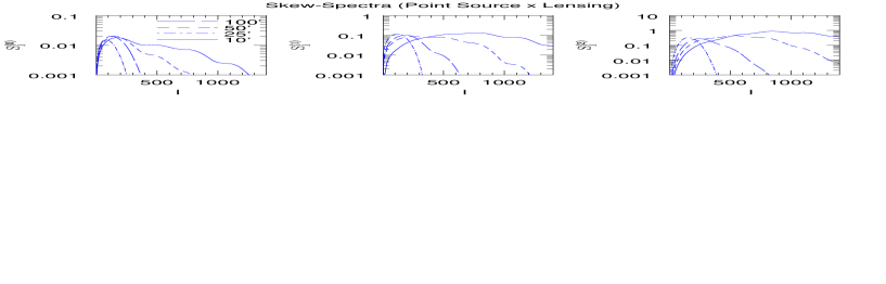
Figure 7: The skew-spectra $S_{l}^{(0)}(\theta_{b}),\;S_{l}^{(1)}(\theta_{b})$ and $S_{l}^{(2)}(\theta_{b})$ for Point-Source$\times$Lensing is plotted as a function of the harmonics $l$. The similarity of the underlying bispectrum for unresolved point-sources and the SZ effect means the shape of resulting skew-spectra are similar.

5 Estimator, Sky Coverage and Error Analysis

The results derived above correspond to a situation in which an all-sky map is available which is free from noise. However, in reality often we have to deal with issues that are related to the presence of a mask and (possibly inhomogeneous) noise. Partial sky coverage introduces mode-mode coupling in the harmonic domain in such a way that individual masked harmonics become linear combinations of all-sky harmonics. The coefficients for this linear transformation depend on specific choice of mask through its own harmonic coefficients. We will devise a method that can be used to correct for this mode-mode coupling based on the Pseudo-${\cal C}_{\ell}$ (PCL) method devised by Hivon et al. (2002) for power spectrum analysis and later developed by Munshi et al. (2011a) for analyzing the skew spectra and the kurt-spectrum (Munshi et al., 2011c).

Consider two generic fields $A({\hat{\Omega}})$ and $B({\hat{\Omega}})$ and denote their harmonic decompositions in the presence of a mask $w({\hat{\Omega}})$ as $\tilde{A}_{lm}$ and $\tilde{B}_{lm}$. Notice that the mask is completely general and our results do not depend on any specific symmetry requirements such as the azimuthal symmetry. The fields $A$ and $B$ may correspond to any of the fields we have considered above. In a generic situation $A$ and $B$ will denote composite fields and the harmonics $A_{lm}$ and $B_{lm}$ will correspond to any of the harmonics listed in Eq.(31) i.e., $[{\Theta}^{2}]_{lm}$,   $[\nabla{\Theta}\cdot\nabla{\Theta}]_{lm}$ and $[\nabla^{2}{\Theta}]_{lm}$:

Mission	$\theta_{b}$	$\sigma_{\rm pix}$	$\Omega_{\rm pix}$	Frequency
Planck	$7.1^{\prime}$	$2.2\times 10^{-6}$	0.0349	143 (GHz)
EPIC	$5.0^{\prime}$	$8.0\times 10^{-9}$	0.002	150 (GHz)

Table 1: Parameters used to compute the skew-spectra and the associated scatter for the two different experiments, ongoing Planck (Planck Collaboration, 2008) and EPIC (Baumann et al., 2009).

$$\tilde{A}_{lm}=\int~{}d{\hat{\Omega}}~{}Y^{*}_{lm}({\hat{\Omega}})~{}[w({\hat{\Omega}})~{}A({\hat{\Omega}})];$$ (32)

$$\tilde{A}_{lm}=\sum_{l_{i}m_{i}}(-1)^{m}~{}I_{ll_{1}l_{2}}\left(\begin{array}[]{ c c c }l_{1}&l_{2}&l\\ m_{1}&m_{2}&-m\end{array}\right)w_{l_{1}m_{1}}A_{l_{2}m_{2}}.$$ (35)

Similar expressions holds for $B$. The above expression relates the masked harmonics denoted by $\tilde{A}_{lm}$ and $\tilde{B}_{lm}$ with their all-sky counterparts $A_{lm}$ and $B_{lm}$ respectively. In their derivation we use the Gaunt integral to express the overlap integrals involving three spherical harmonics in terms of the $3j$ symbols (Edmonds, 1968). The matrix $I_{l_{1}l_{1}l_{3}}$ encodes the overlap integral defined in Eq.(13). The expressions also depend on the harmonics of the mask $w_{lm}$. If we now denote the (cross) power spectrum constructed from the masked harmonics and denote it by $\tilde{S}_{l}(\theta_{b})$ and its all-sky counterpart by $S_{l}(\theta_{b})$ we can write:

$$\tilde{S}_{l}^{A,B}(\theta_{b})={1\over 2l+1}\sum_{m}\tilde{A}_{lm}\tilde{B}^{*}_{lm};\quad\tilde{S}_{l}^{A,B}(\theta_{b})=\sum_{l^{\prime}}M_{ll^{\prime}}S_{l}^{A,B}(\theta_{b});\quad M_{ll^{\prime}}={1\over 2l+1}\sum_{l^{\prime}l^{\prime\prime}}I^{2}_{ll^{\prime}l^{\prime\prime}}|w_{l^{\prime\prime}}|^{2};\quad$$ (36)

$$\hat{S}_{l}^{A,B}(\theta_{b})=\sum_{l^{\prime}}[M^{-1}]_{ll^{\prime}}\tilde{S}_{l^{\prime}}^{A,B}(\theta_{b});\quad\langle\delta\hat{S}_{l}^{A,B}(\theta_{b})\delta\hat{S}_{l^{\prime}}^{A,B}(\theta_{b})\rangle=\sum_{LL^{\prime}}M^{-1}_{lL}\langle\delta\tilde{S}_{L}^{A,B}(\theta_{b})\delta\tilde{S}_{L^{\prime}}^{A.B}(\theta_{b})\rangle M^{-1}_{L^{\prime}l^{\prime}};\quad\langle\hat{S}_{l}^{A,B}(\theta_{b})\rangle=S_{l}^{A,B}(\theta_{b});$$ (37)

$$\delta S_{l}^{A,B}(\theta_{b})=\langle\hat{S}_{l^{\prime}}^{A,B}(\theta_{b})\rangle-S_{l}^{A,B}(\theta_{b});\quad\quad\quad\quad\left\{A,B\right\}\in\left\{{\Theta},{\Theta}^{2},(\nabla{\Theta}\cdot\nabla{\Theta}),\nabla^{2}{\Theta}\right\}.$$ (38)

The final expressions will be independent of the azimuthal quantum number $m$ due to our assumption of isotropy. In the above derivation we have used the orthogonality properties of the $3j$ symbols.

It is interesting to note that the convolved power spectrum estimated from the masked sky is a linear combination of all-sky spectra and depends only on the power spectrum of the mask used. The linear transform is encoded in the mode-mode coupling matrix $M_{ll^{\prime}}$ which is constructed from the knowledge of the power spectrum of the mask. In certain situations where the sky coverage is very restricted the direct inversion of the mode-mixing matrix $M$ may not be possible sue to its singularity and binning may be essential. Based on these results it is possible to define an unbiased estimator that we denote by $\hat{S}_{l}^{A,B}(\theta_{b})$. The noise, due to its Gaussian nature, does not contribute in these estimators which remains unbiased. However, the presence of noise is felt in the increase in the scatter or covariance of these estimators (which can be computed analytically):

$$[\hat{V}_{k}^{(2)}]_{l}=\sum_{l^{\prime}}[M^{-1}]_{ll^{\prime}}[\tilde{V}_{k}^{(2)}]_{l};\quad\quad\langle\delta\hat{V}_{k}^{(2)}\delta\hat{V}_{k^{\prime}}^{(2)}\rangle=\sum_{LL^{\prime}}M^{-1}_{lL}\langle\delta[\tilde{V}_{k}^{(2)}]_{l}\delta[\tilde{V}_{k^{\prime}}^{(2)}]_{l^{\prime}}\rangle M^{-1}_{L^{\prime}l^{\prime}}.$$ (39)

The symbol $S_{l}^{A,A}(\theta_{b})$ denotes the power spectrum of the field $A({\hat{\Omega}})$; $A({\hat{\Omega}})$ is a generic field that are used for the construction of generalized skew-spectra. The derivation of the covariance depends on a Gaussian approximation i.e. we ignore higher-order non-Gaussianity in the fields. ${\cal C}_{l}$ is the ordinary CMB power spectra it also includes the effect of instrumental noise and beam ${\cal C}_{l}(\theta_{b})={\cal C}^{S}_{l}b_{l}^{2}(\theta_{b})+n_{l}$. For a survey with homogeneous noise, we can write ${\cal C}_{l}^{N}=\Omega_{p}\sigma_{N}^{2}$ where $\Omega_{p}$ is the pixel area and $\sigma_{N}$ is the noise r.m.s. In a regime when noise contributions dominate, the MFs can be approximated by a Gaussian approximation. The resulting expressions are listed below:

$$\langle\delta S_{l}^{A,B}(\theta_{b})\delta S_{l^{\prime}}^{A,B}(\theta_{b})\rangle={1\over 2l+1}\left[S_{l}^{A,A}(\theta_{b})\;S_{l}^{B,B}(\theta_{b})+[S_{l}^{A,B}(\theta_{b})]^{2}\right];$$ (40)

$$\langle\delta S_{l}^{A_{1},B_{1}}(\theta_{b})\delta S_{l^{\prime}}^{A_{2},B_{2}}(\theta_{b})\rangle={1\over 2l+1}\left[S_{l}^{A_{1},A_{2}}(\theta_{b})\;S_{l}^{B_{1},B_{2}}(\theta_{b})+S_{l}^{A_{1},B_{2}}(\theta_{b})\;S_{l}^{A_{2},B_{1}}(\theta_{b})\right];\quad$$ (41)

$$\quad\quad\quad\left\{A_{1},B_{1},A_{2},B_{2}\right\}\in\left\{{\Theta},{\Theta}^{2},(\nabla{\Theta}\cdot\nabla{\Theta}),\nabla^{2}{\Theta}\right\}.$$ (42)

In the next section we will provide detailed explicit expressions for various choices of estimators.

The two-to-one estimators are from a family of non-Gaussian estimators. The three-to-one estimator probes the four-point correlation function or equivalently the (angular) trispectrum $T^{l_{1}l_{2}}_{l_{3}l_{4}}(L)$ (Cooray, Li & Melchiorri, 2008). These spectra have been used to probe primordial non-Gaussianity beyond lowest order i.e. to separate contributions from $\tau_{\rm NL}$ and $g_{\rm NL}$. The two-to-two spectrum or the power-spectrum of the squared CMB maps was found to be useful in the context of studies of weak lensing induced CMB non-Gaussianity (Cooray & Kesden, 2003). The next order corrections to the generalized skew-spectra too have been constructed using such an approach (Munshi, Smidt & Cooray, 2010) in the context of studies of MF. The Pseudo-${\cal C}_{l}$ formalism discussed above is useful for constructing a quadruplets of trispectra. The error estimates for these higher order contributions too can be computed using a formalism we outline next.

6 Explicit Expressions for Covariances

As we have already stressed, the estimators we have introduced for the skew-spectra are correlated and do not carry independent information. Their correlation structure depends on the experimental beam, noise and sky-coverage. Just as with non-Gaussianiaty, partial sky coverage also introduces mode-mode coupling. However using the mode-mixing matrix defined in Eq.(36) it is possible to deconvolve the convolved skew-spectra $\tilde{S}_{l}$. In this section, we list the expressions for the co-variance of various estimators for skew-spectra. The variances or the scatter of the skew-spectra defined in Eq.(38) take the following forms:

$$\langle[\delta S_{l}^{\Theta^{2},\Theta}(\theta_{b})]^{2}\rangle\equiv\langle[S_{l}^{\Theta^{2},\Theta}(\theta_{b})]^{2}\rangle-\langle S_{l}^{\Theta^{2},\Theta}(\theta_{b})\rangle^{2}={f_{\rm sky}^{-1}\over 2l+1}\left[S_{l}^{\Theta^{2},\Theta^{2}}(\theta_{b})\;S_{l}^{\Theta,\Theta}(\theta_{b})+[S_{l}^{\Theta^{2},\Theta}(\theta_{b})]^{2}\right],$$ (43)

$$\langle[\delta S_{l}^{\Theta^{2},\nabla^{2}\Theta}(\theta_{b})]^{2}\rangle\equiv\langle[S_{l}^{\Theta^{2},\nabla^{2}\Theta}(\theta_{b})]^{2}\rangle-\langle S_{l}^{\Theta^{2},\nabla^{2}\Theta}(\theta_{b})\rangle^{2}={f_{\rm sky}^{-1}\over 2l+1}\left[S_{l}^{\Theta^{2},\Theta^{2}}(\theta_{b})\;S_{l}^{\nabla^{2}\Theta,\nabla^{2}\Theta}(\theta_{b})+[S_{l}^{\Theta^{2},\nabla^{2}\Theta}(\theta_{b})]^{2}\right],$$ (44)

$$\langle[\delta S_{l}^{\nabla^{2}\Theta,\nabla\Theta\cdot\nabla\Theta}(\theta_{b})]^{2}\rangle\equiv\langle[S_{l}^{\nabla^{2}\Theta,\nabla\Theta\cdot\nabla\Theta}(\theta_{b})]^{2}\rangle-\langle S_{l}^{\nabla^{2}\Theta,\nabla\Theta\cdot\nabla\Theta}(\theta_{b})\rangle^{2}{}$$

$$\quad\quad\quad\quad\quad\quad={f_{\rm sky}^{-1}\over 2l+1}\left[S_{l}^{\nabla^{2}\Theta,\nabla^{2}\Theta}(\theta_{b})\;S_{l}^{\nabla\Theta\cdot\nabla\Theta,\nabla\Theta\cdot\nabla\Theta}(\theta_{b})+[S_{l}^{\nabla^{2}\Theta,\nabla\Theta\cdot\nabla\Theta}(\theta_{b})]^{2}\right].$$ (45)

Here $f_{\rm sky}$ is the fraction of the sky covered. The expressions for the cross-covariances can also be computed using the similar technique. We express the harmonics of the composite fields such as $[\Theta^{2}]_{lm}$, $[\nabla\Theta\cdot\nabla\Theta]_{lm}$ in terms of harmonics of the $[\Theta]_{lm}$ field using the overlap integral. The final equations are derived using Wick’s theorem to simplify the resulting expressions.

$$\langle\delta S_{l}^{\Theta^{2},\Theta}(\theta_{b})\;\delta S_{l}^{\nabla\Theta\cdot\nabla\Theta,\Delta^{2}\Theta}(\theta_{b})\rangle={f_{\rm sky}^{-1}\over 2l+1}\left[[S_{l}^{\Theta^{2},\nabla\Theta\cdot\nabla\Theta}(\theta_{b})][S_{l}^{\Theta,\Delta^{2}\Theta}(\theta_{b})]+[S_{l}^{\Theta,\nabla\Theta\cdot\nabla\Theta}(\theta_{b})][S_{l}^{\Theta^{2},\Delta^{2}\Theta}(\theta_{b})]\right],$$ (46)

$$\langle\delta S_{l}^{\Theta^{2},\Theta}(\theta_{b})\;\delta S_{l}^{\Theta^{2},\Delta^{2}\Theta}(\theta_{b})\rangle={f_{\rm sky}^{-1}\over 2l+1}\left[S_{l}^{\Theta^{2},\Theta^{2}}(\theta_{b})\;S_{l}^{\Theta,\Delta^{2}\Theta}(\theta_{b})+S_{l}^{\Theta^{2},\Theta}(\theta_{b})\;S_{l}^{\Theta^{2},\Delta^{2}\Theta}(\theta_{b})\right],$$ (47)

$$\langle\delta S_{l}^{\nabla\Theta\cdot\nabla\Theta,\Delta^{2}\Theta}(\theta_{b})\;\delta S_{l}^{\Theta^{2},\Delta^{2}\Theta}(\theta_{b})\rangle={f_{\rm sky}^{-1}\over 2l+1}\left[S_{l}^{\Theta^{2},\nabla\Theta\cdot\nabla\Theta}(\theta_{b})\;S_{l}^{\Delta^{2}\Theta,\Delta^{2}\Theta}(\theta_{b})+S_{l}^{\Theta^{2},\Delta^{2}\Theta}(\theta_{b})S_{l}^{\nabla\Theta\cdot\nabla\Theta,\Delta^{2}\Theta}(\theta_{b})\right].$$ (48)

The final expressions that we derive are applicable to near all-sky surveys. When a small portion of the sky is covered a sky patch version of our calculations can be performed using two dimensional Fourier analysis instead of the spherical harmonic analysis that we use here. Some of the terms appearing in these expressions can be expressed in terms of the bispectrum. If we assume that the instrumental noise is Gaussian then there is no contribution from noise in these expressions.

$$S_{l}^{\langle\Theta^{2},\nabla^{2}\Theta\rangle}(\theta_{b})=-\sum_{l_{i}=2}^{l_{\rm max}}l(l+1)\;B_{ll_{1}l_{2}}J_{ll_{1}l_{2}}b_{l}b_{l_{1}}b_{l_{2}},$$ (49)

$$S_{l}^{\langle\Theta,\nabla\Theta\cdot\nabla\Theta\rangle}(\theta_{b})=\sum_{l_{i}=2}^{l_{\rm max}}B_{ll_{1}l_{2}}J_{ll_{1}l_{2}}[l(l+1)+l_{1}(l_{1}+1)-l_{2}(l_{2}+1)]b_{l}b_{l_{1}}b_{l_{2}},$$ (50)

$$S_{l}^{\langle\nabla\Theta\cdot\nabla\Theta,\Delta^{2}\Theta\rangle}(\theta_{b})=-\sum_{l_{i}=2}^{l_{\rm max}}B_{ll_{1}l_{2}}J_{ll_{1}l_{2}}\{l(l+1)[l(l+1)+l_{1}(l_{1}+1)-l_{2}(l_{2}+1)]\}b_{l}b_{l_{1}}b_{l_{2}}.$$ (51)

Notice that these expressions are generic, in that they are derived without any specific assumption about the shape of the bispectrum. The rest of the terms can be expressed in terms of the power spectrum alone. As is common practice in the literature these results ignore all higher order correlation beyond the bispectrum.

$$S_{l}^{\langle\Theta^{2},\nabla\Theta\cdot\nabla\Theta\rangle}(\theta_{b})={1\over 2l+1}\sum_{l_{i}=2}^{l_{max}}\left(\begin{array}[]{ c c c }l_{1}&l_{2}&l\\ 0&0&0\end{array}\right)^{2}I^{2}_{l_{1}l_{2}l}[l(l+1)+l_{1}(l_{1}+1)-l_{2}(l_{2}+1)]({\cal C}_{l_{1}}b_{l_{1}}^{2}+n_{l_{1}})({\cal C}_{l_{2}}b_{l_{2}}^{2}+n_{l_{2}}),$$ (54)

$$S_{l}^{\langle\Theta^{2},\Theta^{2}\rangle}={2\over 2l+1}\sum_{l_{i}=2}^{l_{max}}\left(\begin{array}[]{ c c c }l_{1}&l_{2}&l\\ 0&0&0\end{array}\right)^{2}I^{2}_{l_{1}l_{2}l}({\cal C}_{l_{1}}b^{2}_{l_{1}}+n_{l_{1}})({\cal C}_{l_{2}}b^{2}_{l_{2}}+n_{l_{2}}),$$ (57)

$$S_{l}^{\langle\nabla\cdot\nabla,\nabla\cdot\nabla\rangle}={2\over 2l+1}\sum_{l_{i}=2}^{l_{max}}\left(\begin{array}[]{ c c c }l_{1}&l_{2}&l\\ 0&0&0\end{array}\right)^{2}I^{2}_{l_{1}l_{2}l}[l(l+1)+l_{1}(l_{1}+1)-l_{2}(l_{2}+1)]^{2}({\cal C}_{l_{1}}b^{2}_{l_{1}}+n_{l_{1}})({\cal C}_{l_{2}}b^{2}_{l_{2}}+n_{l_{2}}).$$ (60)

The remaining terms are scaled input power-spectra:

$$S_{l}^{\langle\Theta,\nabla^{2}\Theta\rangle}=-l(l+1)({\cal C}_{l}b_{l}^{2}+n_{l});\quad S_{l}^{\langle\nabla^{2}\Theta,\nabla^{2}\Theta\rangle}=l^{2}(l+1)^{2}({\cal C}_{l}b_{l}^{2}+n_{l});\quad S_{l}^{\Theta,\Theta}=({\cal C}_{l}b_{l}^{2}+n_{l}).$$ (61)

The derivation of these results follow the same general principle that is outlined in §5. These expressions are used to compute the cross-correlation coefficient among various spectra which are defined below:

$$r^{ij}_{l}(\theta_{b})=\langle\delta S_{l}^{(i)}(\theta_{b})\delta S_{l}^{(j)}(\theta_{b})\rangle/\sqrt{\langle[\delta S_{l}^{(i)}(\theta_{b})]^{2}\rangle}\sqrt{\langle[\delta S_{l}^{(j)}(\theta_{b})]^{2}\rangle};\quad\quad i,j\in\{0,1,2\}.$$ (62)

As before, throughout we have ignored the mode-mode coupling. The coefficients of cross-correlation $r_{ij}$ are independent of the sky-coverage $f_{\rm sky}$. The signal to noise for individual modes for a given spectrum on the other hand can be expressed as:

$$[{S/N}]^{(i)}_{l}(\theta_{b})=\sqrt{\langle[S_{l}^{(i)}(\theta_{b})]^{2}\rangle/\langle[\delta S_{l}^{(i)}(\theta_{b})]^{2}\rangle}\quad\quad i\in\{0,1,2\}.$$ (63)

The cumulative $[S/N]=\sum_{l=2}^{l_{\rm max}}[{S/N}]^{(i)}_{l}$ is tabulated for individual experiments in Table-2 for Planck and EPIC.

We have also computed the signal to noise ratio for individual modes using these expressions for various skew spectra. These results are plotted in Figure 9 for EPIC as well as for Planck in Figure (8). The cumulative signal-to-noise as expected is higher for EPIC due to higher sensitivity. The signal to noise for ISW decreases sharply at higher $l$ and peak at lower $l$ on the other hand the signal to noise for SZ and unresolved point sources peak at a much higher angular frequency. Among the three skew-spectra we have considered, the skew spectra $S^{(1)}_{l}(\theta_{b})$ was found to have higher signal to noise compared to $S^{(0)}_{l}(\theta_{b})$ and $S^{(2)}_{l}(\theta_{b})$. While the lowest order skew-spectra $S^{(0)}_{l}(\theta_{b})$ is dominated mostly by cosmic variance the other skew-spectra, $S^{(2)}_{l}(\theta_{b})$ is maximally affected by the instrumental noise. The information content is not independent for the different skew-spectra; their cross-correlation coefficient provides a succinct measure of this lack of dependence.

To correct for the effect of a mask and the noise we will follow the Pseudo-${\cal C}_{\ell}$ (PCL) method devised by Hivon et al. (2002) for power spectrum analysis and later developed by Munshi et al. (2011a) for analyzing the skew spectra and the kurt-spectrum (Munshi et al., 2011c).and the cross-correlation coefficient provides a valuable indicator of their independence.

The signal to noise of estimates of one-point generalised skewness parameters $S^{(i)}=\sum_{l=2}^{l_{\rm max}}(2l+1)S^{(i)}_{l}$ is given by $\left[\sum_{l=2}^{l_{\rm max}}{(2l+1)^{2}\langle[\delta S^{(i)}/S^{(i)}]^{2}\rangle}\right]^{-1/2}$. The corresponding numbers for Planck and EPIC are presented in Table 3.

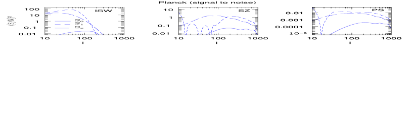
Figure 8: The mode-by-mode signal to noise ratio is depicted for the three skew-spectra, $S^{(0)}_{l}(\theta_{b})$ (left-panel), $S^{(1)}_{l}(\theta_{b})$ (middle-panel) and $S^{(2)}_{l}(\theta_{b})$ (right-panel), as a function of the harmonics $l$. Two different experimental set-ups are considered ongoing experiment Planck (solid curves) and EPIC (dashed-curves). The parameters defining these experiments are summarized in Table 1. We have assumed an all-sky coverage $f_{\rm sky}=1$. The mixed bispectrum that the skew-spectra sample correspond to cross-correlation of lensing and thermal SZ effect. All other source of secondary and primordial non-Gaussianity has been ignored. We use Eq.(40) in conjunction with Eq.(42) in our computation of the scatter.

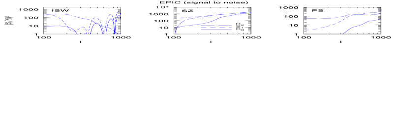
Figure 9: The signal to noise ratio for the three skew-spectra, $S^{(0)}_{l}(\theta_{b})$ (left-panel), $S^{(1)}_{l}(\theta_{b})$ (middle-panel) and $S^{(2)}_{l}(\theta_{b})$ (right-panel), are depicted as a function of the harmonics $l$. Two different experimental set-ups are considered ongoing experiment Planck (solid curves) and EPIC (dashed-curves). The parameters defining these experiments are summarized in Table 1. We have assumed an all-sky coverage $f_{\rm sky}=1$. The mixed bispectrum that the skew-spectra sample correspond to cross-correlation of lensing and thermal SZ effect. All other source of secondary and primordial non-Gaussianity have been ignored.

It is possible to introduce a filter function $w_{l_{1}l_{2}}$ in the definition of the skew-spectra. Choices include, sharp cutoff in the $l$ space to avoid the affect of noise at high $l$, to optimal filters that maximizes the signal to noise for a given resolution $l_{\rm max}$. Clearly such option will invariably improve the statistical significance. The filter functions can be of further interest if the bispectrum is more pronounced for certain triangular configurations. Another potentially useful application of a filter function is to filter out a specific configuration. However in such case the skew-spectra will not have any direct relation with the topological properties of the original map.

7 Conclusion and Discussion

Non-Gaussianity is in itself a poorly defined concept, in that there is no unique approach that can be adopted to describe or parametrize an arbirary form of non-Gaussianity in a complete manner. In order to quantify non-Gaussianity as fully as possible it is therefore essential to deploy a battery of complementary approaches each of which exploits different statistical characteristics. Each such technique will have a unique response to real world issues such as the sky-coverage (observational mask), beam and instrumental noise. Any robust detection therefore will have to involve a simultaneous cross-validation of results obtained from independent methods. The most common characterizations of non-Gaussianity involve studying the bispectrum, which represents the lowest-order departure from Gaussianity; higher order non-Gaussianity can be studied using its higher order analogues i.e. the multi-spectra.

By contrast the topological estimators (MFs) that we have studied here carry information to all orders, though in a collapsed (one-point) form. Analytical results for MFs for a Gaussian field are well understood, and form the basis of non-Gaussianity studies (Tomita, 1986). There have been several previous studies on extraction of the MFs from the CMB data that rely either on simplification of radiative transfer using the Sachs-Wolfe limit (Hikage et al., 2006) or using a perturbative approach based on a series expansion of the MFs that can be studied order by order (Matsubara, 2003, 1994). The MFs have also been studied using elaborate computer-intensive non-Gaussian simulations (Komatsu et al., 2003; Spergel et al., 2007). Most of these studies were done using a specific model of non-Gaussianity, namely the local model of primordial non-Gaussianity which is parametrized by the well known parameter $f_{\rm NL}$.

The main motivation behind the present study has been to to extend such methods to secondary non-Gaussianities which have not been studied before in the context of morphological statistics analytically. The increase in sensitivity of CMB experiments and near all-sky coverage along with wide frequency range means the study of non-Gaussianities will be feasible in the very near future. Moreover, in the currently favoured adiabatic CDM models it is expected that the contribution from primordial non-Gaussianity is negligible and the main contribution to non-Gaussianities comes from secondaries. The secondary non-Gaussianity signal are associated with large scale structure contributions and through various mode coupling effects such as gravitational lensing (Goldberg & Spergel, 1999a, b; Cooray & Hu, 2000). Our primary aim in this work has been to study how well we can probe the secondary signals from mode coupling using morphological descriptors.

One of the main difficulties faced by one-point estimators $S^{(i)}(\theta_{b})$, which also affects the MF-based estimators $V_{k}(\nu)$, is their inability to differentiate among various sources of non-Gaussianity. The triplets of skew spectra $S^{(i)}_{l}(\theta_{b})$ that we have introduced can be used to separate out contributions from various secondaries as well as to probe and constrain any foreground residuals left from the component separation step of the data analysis chain. Generalizing Munshi & Heavens (2010) we have introduce a set of triplets of skew-spectra which can be extracted from any realistic data. These skew-spectra do not compress the available information from a bispectrum to a single number, and their shape can help to distinguish among various sources of non-Gaussianity. Exploiting the perturbative expansion of the MFs, we showed that at the leading order of non-Gaussianity the MFs are completely specified by the knowledge of the bispectrum. Our results are most naturally defined in the harmonic domain. Comparison of MFs extracted using harmonic approach can be cross-compared with more traditional approach in the real space as an useful consistency check.

The methods based on the skew-spectra that we have presented are simple to implement once the derivative fields $[\nabla\Theta\cdot\nabla\Theta]$ or $[\nabla^{2}\Theta]$ are constructed. We have shown that this can be implemented in a model-independent way. Our method is based on a Pseudo-${\cal C}_{l}$ approach (Hivon et al., 2002) and can handle arbitrary sky coverage and inhomogeneous noise distributions. The Pseudo-${\cal C}_{\ell}$ approach is well understood in the context of power spectrum studies, and its variance or scatter can be computed analytically. We provide generic analytical results for the computation of scatter around individual estimates. We also provide detailed predictions on how they are cross-correlated. In our method, it is possible indeed to go beyond the lowest level in non-Gaussianity to include the contribution from trispectrum. The main contributions in frequency-cleaned CMB maps will be from lensing of the CMB, though it is expected that such corrections will be sub dominant at least in the context of CMB data analysis.

(Planck,EPIC)	SZ	ISW	PS
$\left({S/N}\right)$	$(5.0,1137.4)$	$(1.0,216.0)$	$(0.5,209.0)$
$\left({S/N}\right)$	$(24.0,1354.9)$	$(62.2,420.3)$	$(4.3,552.0)$
$\left({S/N}\right)$	$(19.7,1328.8)$	$(31.8,246.5)$	$(1.7,421.0)$

Table 2: The cumulative signal to noise (S/N) for Planck and EPIC surveys, are shown for the three one-point skew-spectra. Parameters used to compute the skew-spectra and the associated scatter for the two different experiments, ongoing Planck (Planck Collaboration, 2008) and EPIC (Baumann et al., 2009).

(Planck,EPIC)	SZ	ISW	PS
$\left({S/N}\right)$	$(3.8,503.2)$	$(0.3,39.3)$	$(0.4,53.4)$
$\left({S/N}\right)$	$(5.8,1299.0)$	$(6.4\times 10^{-2},70.9)$	$(0.6,529.1)$
$\left({S/N}\right)$	$(1.2,625.8)$	$(1.4\times 10^{-2},21.1)$	$(0.1,178.2)$

Table 3: The cumulative signal to noise (S/N) for Planck and EPIC surveys for the one-point cumulants $S^{(i)}({\hat{\Omega}})$, defined in Eq.(63), are shown for each skew-spectra. Parameters used to compute the skew-spectra and the associated scatter for the two different experiments, ongoing Planck (Planck Collaboration, 2008) and EPIC (Baumann et al., 2009). We have assumed $f_{\rm sky}=1$ in our calculations.

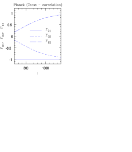
Figure 10: Same as the previous Figure but for Planck noise. The expression for scatter Eq.(43)-Eq.(45)and cross-correlation Eq.(46)-Eq.(48) has two contributions. In each of these expressions there are terms which depend on the bispectrum and there are terms which can constructed from power spectrum alone. For Planck noise we found that the expressions for the scatter as well as the cross-correlation are entirely dominated by the terms which depend only on the power spectrum thus making the coefficient $r_{ij}$ independent of the type of underlying bispectrum.

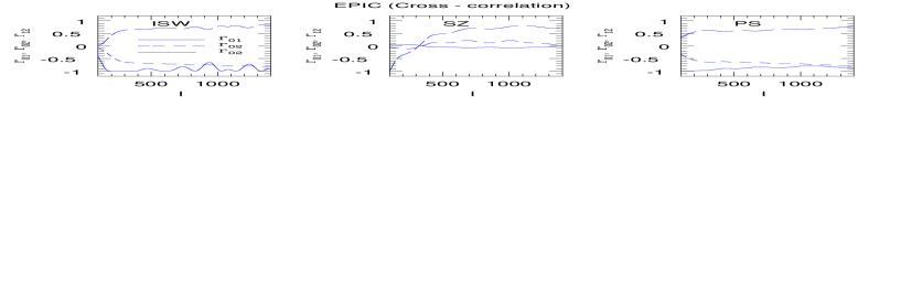
Figure 11: The information content of the skew-spectra are not completely independent. The level of cross-correlation among various estimator is encoded in the coefficient of cross-correlations $r_{ij}$ defined in Eq.(62). The cross-correlation coefficient $r_{01}$, $r_{02}$ and $r_{12}$ are plotted as a function of harmonics $l$. The noise level correspond to that of EPIC (see Table 1). The correlation structure refelects the underlying spectra $\beta_{l}$ as well as the level of noise. The cross-correlation is similar for SZ and PS.

We conclude by pointing out that the MFs do not probe the full bispectrum, but involve only weighted sums of modes and are thus equivalent to the three generalised skewness parameters we have used. We have also defined three generalized skew-spectra associated with each of these skewness parameters. In this sense, the study of these skew-spectra can replace the study of MFs. The skew-spectra we have introduced can all be probed for arbitrary mask and noise. Ubiased estimators can also be constructed which can work in the presence of partial sky coverage and inhomogeneous noise. Their variance can also be computed analytically; thereby avoiding the use of non-Gaussian Monte-Carlo simulations completely. Finally, the MFs can be constructed from the knowledge of generalized skew-spectra and can be compared with the results from real space analysis. The triplets of generalized skew-spectra can be used to separate individual components of NGs using their shape information. From our analytical results of cross-correlation, we find that in the absence of noise, e.g. experiments such as EPIC, the skew-spectra are highly correlated, more so for higher $l$ values. The correlation coefficients are typically in the range $r=0.5-1$ for a Planck type experiment. The cumulative signal-to-noise ratio, in a Planck type experiment, for bispectrum corresponding to the ISW and SZ and lensing cross-correlation reaches ${\cal O}(10)$. An improvement of about two orders of magnitude can be expected with experiments such as EPIC.

Throughout we have ignored the presence of primordial non-Gaussianity which is expected to be subdominant. Nevertheless, it can be incorporated. Individual skew-spectra from different underlying bispectrum can essentially be combined to construct the total skew-spectra which means that our results can straightfowardly be generalised to incorporate specific models of primordial non-Gaussianity.

The generic results derived here are also applicable to other areas in cosmology and have indeed been explored recently. Examples include the analysis of galactic redshift surveys (Pratten & Munshi, 2012), weak lensing surveys (Munshi et al., 2012a) and the frequency cleaned SZ maps (Munshi et al., 2012b). The results presented here can be extended beyond the analysis of temperature maps, e.g. to analyze polarisation maps, by extending the spin-$0$ calculations to spin-$2$. Such results can furnish useful probes for tje characterization of morphology of reionization in three dimensions.

A few comments are in order about the comparison of our estimators with the so-called optimal estimators. The motivation to construct an optimal estimator is to improve the signal-to-noise of detection which is important in case of weak signals such as the primordial non-Gaussianity. The main motivation in this paper has been to reconstruct the topological properties of the CMB map going beyond Gaussianity, in the harmonic domain; in particular due to the contributions from secondary lensing cross-correlation which will be detected with high signal to noise with the proposed CMB surveys such as EPIC.

In addition to the primary and secondary non-Gaussianity, cosmic defects such as textures or cosmic strings (Albrecht, Battey & Robinson, 1999; Cruz etal., 2007; Regan & Shellard, 2010) also leave non-Gaussian footprints in CMB maps which can be detected by the change in topological nature of the maps. The estimators we have presented here may have relevance in such investigations. A detailed study will be presented elsewhere.

At the level of the bispectrum the effect of lensing can only be studied through its cross-correlation with other secondaries. However weak lensing is also independently responsible for a next order correction to MFs through its effect on the trispectrum; the signal-to-noise is expected to be low.

The signal-to-noise of the skew-spectra for secondary-lensing cross-correlation bispectrum is comparable to that of the skew-spectra of frequency-cleaned SZ maps (Munshi et al., 2012b). However the secondary skew-spectra are much higher compared to skew-spectra associated with primary skew-spectra unless we assume a rather high value for the $f_{\rm NL}$.

8 Acknowledgements

DM and PC acknowledges support from STFC standard grant ST/G002231/1 at the School of Physics and Astronomy at Cardiff University where this work was completed. DM would like to thank Joseph Smidt, Geraint Pratten, Asantha Cooray, Shahab Joudaki and Erminia Calabrese for very useful discussions.

Appendix A Spherical Harmonics

The completeness relationship for the spherical harmonics $Y_{lm}({\hat{\Omega}})$ is given by:

$$\sum_{lm}Y_{lm}({\hat{\Omega}})Y^{*}_{lm}({\hat{\Omega}}^{\prime})=\delta_{2\rm D}({\hat{\Omega}}-{\hat{\Omega}}^{\prime}).$$ (64)

The orthogonality relationship is as follows:

$$\int d{\hat{\Omega}}\;Y_{lm}({\hat{\Omega}})Y^{*}_{l^{\prime}m^{\prime}}({\hat{\Omega}})=\delta^{\rm K}_{ll^{\prime}}\delta^{\rm K}_{mm^{\prime}}.$$ (65)

Here $\delta_{2\rm D}$ and $\delta^{\rm K}$ represents the Dirac’s 2-dimensional delta function and Kroneker’s Delta function resepctively.

Appendix B 3j Symbols

The following properties of $3j$ symbols were used to simplify various expressions.

$$\sum_{l_{3}m_{3}}(2l_{3}+1)\left(\begin{array}[]{ c c c }l_{1}&l_{2}&l_{3}\\ m_{1}&m_{2}&m_{3}\end{array}\right)\left(\begin{array}[]{ c c c }l_{1}&l_{2}&l\\ m_{1}^{\prime}&m_{2}^{\prime}&m\end{array}\right)=\delta^{K}_{m_{1}m_{1}^{\prime}}\delta^{K}_{m_{2}m_{2}^{\prime}};$$ (70)

$$\sum_{m_{1}m_{2}}\left(\begin{array}[]{ c c c }l_{1}&l_{2}&l_{3}\\ m_{1}&m_{2}&m_{3}\end{array}\right)\left(\begin{array}[]{ c c c }l_{1}&l_{2}&l_{3}^{\prime}\\ m_{1}&m_{2}&m_{3}^{\prime}\end{array}\right)={\mathcal{\delta}^{K}_{l_{3}l_{3}^{\prime}}\delta^{K}_{m_{3}m_{3}^{\prime}}\over 2l_{3}+1};$$ (75)

$$(-1)^{m}\left(\begin{array}[]{ c c c }l&l&l^{\prime}\\ m&-m&0\end{array}\right)={(-1)^{l}\over\sqrt{(2l+1)}}\delta^{K}_{l^{\prime}0};$$ (78)

$$\int d{\hat{\Omega}}Y_{lm}({\hat{\Omega}})Y_{l^{\prime}m^{\prime}}({\hat{\Omega}})Y_{LM}({\hat{\Omega}})=\sqrt{(2l+1)(2l+1)(2L+1)\over 4\pi}\left(\begin{array}[]{ c c c }l&l^{\prime}&L\\ m&m^{\prime}&M\end{array}\right)\left(\begin{array}[]{ c c c }l&l^{\prime}&L\\ 0&0&0\end{array}\right).$$ (83)

References

- Acquaviva et al. (2003) Acquaviva V., Bartolo N., Matarrese S., Riotto A., 2003, Nucl. Phys. B667, 119
- Adler (1981) Adler R. J., 1981, The Geometry of Random Fields, Chichester: Wiley
- Albrecht, Battey & Robinson (1999) Albrecht A., Battye R.A., Robinson J., PRD, 1999, 59, 023508
- Babich (2005) Babich D., 2005, Phys. Rev. D72, 043003
- Bartolo, Matarrese & Riotto (2006) Bartolo N., Matarrese S., Riotto A., 2006, JCAP, 06, 024
- Bartolo et al. (2004) Bartolo N., Komatsu E., Matarrese S., Riotto A., 2004, Phys.Rept. 402, 103
- Baumann et al. (2009) Baumann D. et al. [CMBPol Study Team Collaboration], AIP Conf. Proc.2009, 1141, 10 arXiv:0811.3919
- Birkinshaw (1999) Birkinshaw M., Phys.Rept, 1999, 310, 97
- Bock et al. (2008) Bock J. et al. 2008, arXiv:0805.4207
- Bock et al. (2009) Bock J. et al. 2009, arXiv:0906.1188
- Boughn & Crittenden (2004) Boughn S., Crittenden R., 2004, Nature, 427, 45
- Calabrese et al. (2010) Calabrese E., Smidt J., Amblard A., Cooray A., Melchiorri A., Serra P., Heavens A., Munshi D. 2010, PRD, 81, 3529
- Canavezes et al. (1998) Canavezes A., et al., 1998, MNRAS, 297, 777
- Castro et al. (2004) Castro P. G. Phys.Rev. 2004, D67, 044039
- Chen (2010) Chen X., Advances in Astronomy, 2010, 2010:638979
- Coles (1988) Coles P., 1988, MNRAS, 234, 509
- Cooray & Hu (2000) Cooray A.R., Hu W., 2000, ApJ, 534, 533
- Cooray (2001a) Cooray A., 2001a, PRD, 64, 043516
- Cooray (2001b) Cooray A., 2001b, PRD, 64, 063514
- Cooray & Seth (2002) Cooray A , Sheth R., 2002, Phys.Rept., 372, 1,
- Cooray (2002) Cooray A., 2002, PRD, 65, 103510
- Cooray & Kesden (2003) Cooray A., Kesden M., 2003, New Astron., 8, 231
- Cooray (2006) Cooray A., 2006, PRL, 97, 261301
- Cooray, Li & Melchiorri (2008) Cooray A., Li C., Melchiorri A., 2008, PRD, 77,103506
- Copi et al. (2007) Copi C., Huterer D., Schwarz D., Starkman G., 2007, PRD, 75, 023507
- The COrE Collaboration (2012) The COrE Collaboration, 2011arXiv1102.2181
- Cruz etal. (2007) Cruz, M., Turok N., Vielva P., Martínez-González E., Hobson M., Science 318 (5856) 1612
- Edmonds (1968) Edmonds, A.R., Angular Momentum in Quantum Mechanics, 2nd ed. rev. printing. Princeton, NJ:Princeton University Press, 1968.
- Falk et al. (1993) Falk T., Madden R., Olive K.A., Srednicki M., 1993, Phys. Lett. B318, 354
- Ferreira, Magueijo & Gorski (1998) Ferreira P.G., Magueijo J. & Gorski K.M., ApJ, 1998, 503, 1
- Gangui et al. (1994) Gangui A., Lucchin F., Matarrese S., Mollerach S., 1994, ApJ, 430, 447
- Gleser et al. (2006) Gleser L., Nusser A., Ciardi B., Desjacques V., 2006, MNRAS, 370, 1329
- Goldberg & Spergel (1999a) Goldberg D.M., Spergel D.N., 1999a, PRD, 59, 103001
- Goldberg & Spergel (1999b) Goldberg D.M., Spergel D.N., 1999b, PRD, 59, 103002
- Gott et al. (1986) Gott J. R., Mellot A. L., Dickinson M., 1986, ApJ., 306, 341
- Gott et al. (1989) Gott J. R., et al., 1989, ApJ., 340, 625
- Gott et al. (1990) Gott J. R., et al., 1990, ApJ., 352
- Gott et al. (1992) Gott J. R., Mao S., Park C., Lahav O., 1992, ApJ., 385, 26
- Hadwiger (1959) Hadwiger H., 1959, Normale Koper im Euclidschen raum und ihre topologischen and metrischen Eigenschaften, Math Z., 71, 124
- Hanson & Lewis (2009) Hanson F.K., Lewis A., 2009, PhRvD, 80, 063004
- Hikage et al. (2002) Hikage C., et al., 2002, Publ. Astron. Soc. Jap., 54, 707
- Hikage et al. (2006) Hikage C., Komatsu E., Matsubara T., 2006, ApJ., 653, 11
- Hikage et al. (2008) Hikage C., et al., 2008, MNRAS, 389, 1439
- Hikage et al. (2008) Hikage C., et al., MNRAS, 2008, 385, 1613
- Hikage, Komatsu & Mastubara (2006) Hikage C., Komatsu E., Matsubara T., 2006, Astrophys. J., 653, 11
- Hinsaw et al. (1995) Hinsaw G., Banday A.J., Bennett C.L., Gorski K.M., Kogut A., 1995, ApJ, 446, 67
- Hivon et al. (2002) Hivon E., Górski K. M., Netterfield C. B., Crill B. P., Prunet S., Hansen F., 2002, ApJ, 567, 2
- Hoftuft et al. (2009) Hoftuft J., Eriksen H.K., Banday A.J., Gorski K.M., Hansen F.K., Lilje P.B., 2009, ApJ, 699, 985
- Hu, Scott & Silk (1994) Hu W., Scott D., Silk J., 1994, PRD, 49, 648
- Joudaki et al. (2010) Joudaki S., Smidt J., Amblard A., Cooray A., 2010, JCAP, 08(2010)027
- Kaminkowski & Spergel (1994) Kaminkowski M., Spergel D., 1994, ApJ, 432, 7
- Kamionkowski, Smith & Heavens. (2011) Kamionkowski M., Smith T.L., Heavens A., 2011, PRD, 83, 023007
- Kerscher et al. (2001) Kerscher M., et al., 2001, A&A., 373, 1
- Komatsu et al. (2003) Komatsu E., et al., 2003, ApJS, 148, 119
- Kofman & Starobinsky (1985) Kofman L.A., Starobinsky, 1985, Sov. Astro., Let., 11, 271
- Larson et al. (2011) Larson D. et al, ApJS, 2011, 192, 16
- Luminet et al. (2003) Luminet J.P., Weeks J., Riazuelo A., Lehoucq R., Uzan J.P., Nature, 2003, 425, 593
- Maldacena (2003) Maldacena J.M., 2003, JHEP, 05, 013
- Martinez-Gonzaléz, Sanz, Silk (1990) Martinez-Gonzaléz E., Sanz J.-L, Silk J., 1990, ApJ, 355, L5
- Matsubara (1994) Matsubara T., 1994, ApJ, 434, L43
- Matsubara (1995) Matsubara T., 1995, ApJS., 101, 1
- Matsubara & Jain (2001) Matsubara T., Jain B., 2001, ApJ, 552, L89.
- Matsubara (2002) Matsubara T., 2002, arXiv:astro-ph/0006269v2
- Matsubara (2003) Matsubara T., 2003, ApJ, 584, 1
- Matsubara (2010) Matsubara T., 2010, PRD, D81, 083505
- Matsubara & Yokohama (1996) Matsubara T., Yokohama J., 1996, ApJ, 463
- Matsubara (2010) Matsubara T., 2010, PRD, D81, 083505
- Matsubara and Jain (2001) Matsubara T., Jain B., 2001, ApJ, 552, L89
- Melott (1990) Melott A. L., 1990, Phys. Rep., 193, 1
- Moore et al. (1992) Moore B., et al., 1992, MNRAS, 256, 477
- Mollerach et al. (1995) Mollerach S., Gangui A., Lucchin F., Mataresse S., 1995, ApJ, 453, 1
- Mukhanov, Feldman & Bandenberger (1992) Mukhanov V.F., Feldman H.A., Bandenberger R.H., 1992, PRD, 215, 203
- Munshi, Souradeep & Starobinsky (1995) Munshi D., Souradeep T., Starobinsky, ApJ, 1995, 454, 552
- Munshi, Melott & Coles (2000) Munshi D., Melott A.L., Coles P., 2000, MNRAS, 311, 149.
- Munshi & Heavens (2010) Munshi D., Heavens A. 2010, MNRAS, 401, 2406
- Munshi, Smidt & Cooray (2010) Munshi D., Smidt J., Cooray A., arXiv:1011.5224
- Munshi et al. (2011) Munshi D., Heavens A., Cooray A., Smidt J., Coles P., Serra P., 2011, MNRAS, 412, 1993
- Munshi et al. (2011a) Munshi D., Valageas P., Cooray A., Heavens A., 2011a, MNRAS, 414, 3173
- Munshi et al. (2011b) Munshi D., Coles P., Cooray A., Heavens A., Smidt J., 2011b, MNRAS, 410, 1295
- Munshi et al. (2011c) Munshi D., Smidt J., Heavens A., Coles P., Cooray A., 2011c, MNRAS, 411, 2241
- Munshi et al. (2011d) Munshi D., Kitching T., Heavens A., Coles P., MNRAS, 2011d, 416, 629
- Munshi et al. (2012a) Munshi D., van Waerbeke L., Smidt J., Coles P., MNRAS, 2012a, 419, 536
- Munshi et al. (2012b) Munshi D., Smidt J., Joudaki S., Coles P., MNRAS, 2012b, 419, 138
- Natoli et al. (2010) Natoli P., et al., arXiv:0905.4301
- Novikov, Schmalzing and Mukhanov (2000) Novikov D., Schmalzing J., Mukhanov V. F., 2000, Astron. Astrophys., 364
- Park et al. (2005) Park C., et al., 2005, Astrophys. J., 633, 11
- Planck Collaboration (2008) Planck Collaboration, arXiv:0811.3919
- Pratten & Munshi (2012) Pratten G., Munshi D., 2012, MNRAS, 423, 3209
- Regan & Shellard (2010) Regan, D. M., Shellard, E. P. S., 2010, PRD, 82, 063527
- Roukemia et al. (2004) Roukemia B.F., Lew B., Cechowska M., Marecki A., Bajtlik S., 2004, A&A, 423, 821
- Sahni, Sathyaprakash & Shandarin (1998) Sahni V., Sathyaprakash B.S., Shandarin S.F., ApJ., 1998, 495, L5.
- Sato et al. (2001) Sato J., et al., 2001, ApJ, 421, 1
- Salopek & Bond (1990) Salopek D. S., Bond J. R., 1990, PhRvD, 42, 3936
- Salopek & Bond (1991) Salopek D. S., Bond J. R., 1991, PhRvD, 43, 1005
- Schmalzing & Górski (1998) Schmalzing J., Górski K. M., 1998, MNRAS, 297, 355
- Schmalzing & Diaferio (2000) Schmalzing J., Diaferio A., 2000, MNRAS, 312
- Smidt (2010) Smidt J., Joudaki S., Serra P., Amblard A., Cooray A., 2010, PhRvD, 81, 123528
- Smith, Zahn & Dore (2007) Smith K.M., Zahn O., Dore O., 2007, Phys. Rev. D, 76, 043510
- Spergel et al. (2007) Spergel D.N. et al., 2007, ApJS, 170, 377
- Szapudi & Szalay (1999) Szapudi I., Szalay A.S., ApJ., 1999, 515, L43
- Taruya et al. (2002) Taruya A., et al., 2002, ApJ, 571, 638
- Tomita (1986) Tomita H., 1986, Progr. Theor. Phys., 76, 952
- Verde & Spergel (2002) Verde L., Spergel D.N., PRD, 65, 043007