Finite frequency noise for edge states at filling factor $\nu=2/5$

Abstract

We investigate the properties of the finite frequency noise in a quantum point contact geometry for the fractional quantum Hall state at filling factor $\nu=2/5$. The results are obtained in the framework of the Wen’s hierarchical model. We show that the peak structure of the colored noise allows to discriminate among different possible excitations involved in the tunneling. In particular, optimal values of voltage and temperature are found in order to enhance the visibility of the peak associated with the tunneling of a 2-agglomerate, namely an excitation with charge double of the fundamental one associated to the single quasiparticle.

I Introduction

The Fractional Quantum Hall Effect (FQHE) DasSarma97 is one of the most remarkable examples of strongly correlated electron system. Since its discovery it has been subject on an intense study both from the theoretical and the experimental point of view, with the aim of providing an unified picture of the plethora of different observed values of filling factor $\nu$. Tsui99 A suitable theoretical framework for the description of these states is provided by the theory of edge states Wen95 . For the Laughlin series Laughlin83 at $\nu=1/(2n+1)$ ($n\in\mathbb{Z}$) a chiral Luttinger Liquid theory described in terms of a single bosonic mode was proposed. Wen90 For the more general Jain series Jain89 with $\nu=p/(2np+1)$ ($p\in\mathbb{Z}$) a possible extension has been proposed by X. G. Wen Wen92 considering $|p|-1$ additional hierarchical fields, propagating with finite velocity along the edge.

Noise experiments in the Quantum Point Contact (QPC) geometry Chang03 have been crucial to demonstrate the existence of the peculiar fractionally charged excitations predicted by the theoretical models. Laughlin83 In particular it was proved that, for the Jain sequence, the elementary quasiparticle (qp) charge is given by $e^{*}=e/(2np+1)$. dePicciotto97 ; Saminadayar97 ; Reznikov99 More recently some intriguing transport experiments have been performed on a QPC at very low temperature and extremely weak backscattering for various filling factors showing a change in the power-law of the backscattering current as a function of temperature and an enhancing of the effective tunneling charge, as extracted from the noise. Chung03 ; Bid09 ; Dolev10 In order to explain both these unexpected behaviors we observed that propagating neutral modes could crucially modify the scaling dimensions of operators leading to a crossover in the relevance of the tunneling process according to measurements.Ferraro08 ; Ferraro10a ; Ferraro10b ; Ferraro10c ; Carrega11

The symmetrized noise at finite frequency Rogovin74 represents an important tool to characterize the predicted crossover phenomenology, complementary and alternative to current and zero frequency noise. From the experimental point of view, measurements of colored noise have been carried out for a QPC in a 2D electron gas at zero magnetic field Zakka07 . Nevertheless, great efforts are devoted to extend the observations to more interesting cases including the FQH regime. From a theoretical point of view, the colored noise was investigated for the Laughlin sequence Chamon95 ; Chamon96 and also for more exotic states like $\nu=5/2$. Bena06 ; Carrega12 In these cases, much of the relevant physics occurs at frequencies close to Josephson frequencies multiple of $\omega_{0}=e^{*}V/\hbar$, ($e^{*}$ the charge of the elementary excitation) that is in the range of GHz for external bias $V$ in the range of $\mu$V. These values, although high, should be experimentally observable.

In this paper we will discriminate among the different tunneling charges involved in the transport, being their contributions resolved at different frequencies. We will focus on the edge state at $\nu=2/5$ where only two bosonic fields, one charged and one neutral, are involved. Wen95 We will demonstrate the necessity to consider voltages larger than the neutral modes cut-off frequency, in order to efficiently detect the presence of the 2-agglomerate.

The paper is divided as follows. In Sec. II we recall the Wen’s model for the description of the FQH state at $\nu=2/5$. In Sec. III we provide the expression for the backscattering current and noise in terms of the tunneling rates. In Sec. IV we analyze the scaling behaviors for various energy regimes. In Sec. V we present the finite frequency noise peak structure for $\nu=2/5$ as a function of the bias voltage in order to determine the optimal values of the physical parameters to observe the $2$-agglomerate peak. Sec. VI is devoted to the conclusions.

II The model

We consider infinite edge states of an Hall bar in the Jain sequence at filling factor $\nu=p/(2np+1)$. Jain89 We focus on the case $\nu=2/5$ ($n=1$ and $p=2$), described by the Lagrangian density Wen95 ; Ferraro10b ($\hbar=1$)

$$\mathcal{L}=\frac{5}{8\pi}\partial_{x}\varphi^{\rm{c}}\left(\partial_{t}-v_{\rm{c}}\partial_{x}\right)\varphi^{\rm{c}}+\frac{1}{8\pi}\partial_{x}\varphi^{\rm{n}}\left(\partial_{t}-v_{\rm{n}}\partial_{x}\right)\varphi^{\rm{n}},$$ (1)

with $v_{\rm{c}}$ the propagation velocity of the charged bosonic mode $\varphi^{\rm{c}}$ and $v_{\rm{n}}$ the one of the neutral bosonic mode $\varphi^{\rm{n}}$. The electron number density of the edge depends on the charged field only, via the relation $\rho(x)=\partial_{x}\varphi^{\rm{c}}(x)/2\pi$. Due to this fact the charge mode velocity is affected by Coulomb interactions, leading to the reasonable assumption $v_{\rm{c}}\gg v_{\rm{n}}$.Levkinskyi08 ; Levkinskyi09 ; Ferraro08 From (1) one can note that the neutral mode co-propagates with respect to the charged one as typical of the states with $p>0$. Wen95 The commutators of the bosonic fields are $[\varphi^{\rm{c/n}}(x),\varphi^{\rm{c/n}}(y)]=i\pi\nu_{\rm{c/n}}\mathrm{sgn}(x-y)$ with $\nu_{\rm{c}}=2/5$ and $\nu_{\rm{n}}=2$.

We consider a generic $m$-agglomerate annihilation operator with charge $e^{*}_{m}=(em\nu_{c})/2=me^{*}$ with $e^{*}=e/5$ the charge of the elementary excitation, namely the single-quasiparticle (qp) ($e$ the electron charge). It can be written as

$$\Psi^{(m,j)}(x,t)=\frac{\mathcal{F}^{(m,j)}}{\sqrt{2\pi a}}e^{i\left(\frac{m}{2}\varphi^{\mathrm{c}}(x,t)+\frac{j}{2}\varphi^{\mathrm{n}}(x,t)\right)}$$ (2)

where $a$ is a finite length cut-off, $m\in\mathbb{N}$ is related to the charge of the excitation and the additional quantum number $j\in\mathbb{Z}$ plays a role analogous to the isospin and is necessary in order to provide the proper fractional statistics. Ferraro10c Note that for a given quasiparticle excitation the integer $m$ and $j$ must have the same parity. The Klein factors $\mathcal{F}^{(m,j)}$ are ladder operators necessary in order to change the particle numbers of the $m$-agglomerate and to provide the proper statistical properties between excitations. Ferraro10a ; Ferraro10c From the long time limit of the two-point imaginary time Green’s function $\mathcal{G}^{(m,j)}(\tau)=\left\langle T_{\tau}\Psi^{(m,j)}(0,\tau){\Psi^{(m,j)}}^{\dagger}(0,0)\right\rangle$ calculated at $x=0$ and at zero temperature Kane92 , one can extract the scaling dimension of the $m$-agglomerate

$$\Delta^{(m,j)}=\frac{1}{2}\left[\nu_{\mathrm{c}}\left(\frac{m}{2}\right)^{2}+\nu_{\mathrm{n}}\left(\frac{j}{2}\right)^{2}\right].$$ (3)

For energies higher than the typical neutral mode bandwidth $\omega_{\mathrm{n}}=v_{\mathrm{n}}/a$ the neutral mode contribution to the dynamics saturates and one has the effective scaling dimension Ferraro08 ; Ferraro10a

$$\tilde{\Delta}^{(m,j)}=\frac{1}{2}\nu_{\mathrm{c}}\left(\frac{m}{2}\right)^{2}$$ (4)

that only depends on the charged sector of the theory. From now on the correspondent charged mode bandwidth $\omega_{\mathrm{c}}=v_{\mathrm{c}}/a$ is assumed as the greatest energy scale of the system.

Note that the above scaling dimension could be strongly affected by interaction with the external environment Rosenow02 ; Papa04 ; Mandal02 ; Yang03 ; Cuniberti97 ; Ferraro08 ; Carrega11 ; Braggio12 , nevertheless in this paper, for sake of simplicity, we only consider the standard unrenormalized case.

III Transport properties

The tunneling through the QPC at $x=0$ of a generic $m$-agglomerate between the $R$ and $L$ edges of the Hall bar, is described by the Hamiltonian $H^{(m)}_{T}=\textbf{t}_{m}\Psi^{(m)}_{R}(0){\Psi_{L}^{(m)}}^{\dagger}(0)+{\rm h.c.}$, where $\Psi^{(m)}_{R}$ ($\Psi^{(m)}_{L}$) is the $m$-agglomerate annihilation operator. From equation (3) it is easy to note that the more relevant single-qps ($m=1$) are the ones with $j=\pm 1$ ($\Delta^{(1,\pm 1)}=3/10$), while among all the $2$-agglomerate ($m=2$) we consider the one with $j=0$ ($\Delta^{(2,0)}=1/5$). All the other operators with the same charge (same $m$) and different $j$ are less relevant in the renormalization group sense and give a negligible contribution to the transport properties with respect to the considered one. Ferraro08 From now on, for notational convenience, we will omit the index $j$ where not necessary.

The tunneling amplitudes $\textbf{t}_{m}$ depend, in general, on the geometry of the constriction, and can be energy dependent. Chang03 In the following they will be assumed as $m$-dependent constants in order to make the discussion clearer and to restrict the number of free parameters of the theory. The total tunneling Hamiltonian will consist of the sum over all possible $m$-agglomerate $H_{T}=\sum_{m}H_{T}^{(m)}$.

In the following we will focus on the weak tunneling regime. At lowest order in the tunneling Hamiltonian the backscattering current of the $m$-agglomerate $I^{(m)}_{B}$ and the finite frequency symmetrized noise $S_{B}^{(m)}(\omega)$ can be written in terms of the tunneling rates Rogovin74 . By using the detailed balance relation the current is Ferraro10a ($k_{B}=1$)

$$I^{(m)}_{B}(\omega_{0})=me^{*}\left(1-e^{-m\omega_{0}/T}\right)\mathbf{\Gamma}^{(m)}(\omega_{0})\,,$$ (5)

with tunneling rate

$$\mathbf{\Gamma}^{(m)}(E)=|\textbf{t}_{m}|^{2}\!\int^{+\infty}_{-\infty}\!\!\!dte^{imEt}G^{<}_{m,R}(0,-t)G^{>}_{m,L}(0,t)\,.$$ (6)

Here, $\omega_{0}=e^{*}V$ is the Josephson frequency associated to the single-qp with $V$ the bias. The correlators $G_{m,l}^{>}(0,t)=\langle\Psi^{(m)}_{l}(0,t)\Psi^{(m)\dagger}_{l}(0,0)\rangle=(G^{<}_{m,l}(0,t))^{*}$ are the two point Green’s functions of the $m$-agglomerate operators on the edge $l=R,L$.

The noise spectral density is

$$S_{B}^{(m)}(\omega)=\int_{-\infty}^{+\infty}dt\,e^{i\omega t}S_{B}^{(m)}(t)\,,$$ (7)

where

$$S_{B}^{(m)}(t)=\left[\langle\delta I^{(m)}_{B}(t)\delta I^{(m)}_{B}(0)\rangle+\langle\delta I^{(m)}_{B}(0)\delta I^{(m)}_{B}(t)\rangle\right]\,,$$ (8)

with $\delta I^{(m)}_{B}$ the fluctuations of the current with respect to the average.

Recalling the definition of the tunneling rate in (6) one has

$$S_{B}^{(m)}(\omega)=(me^{*})^{2}\sum_{\varepsilon,\eta=\pm}\left[\mathbf{\Gamma}^{(m)}(\varepsilon\omega/m+\eta\omega_{0})\right]\,,$$ (9)

or, equivalently, in terms of the backscattering current

$$S_{B}^{(m)}(\omega) = me^{*}\sum_{\varepsilon=\pm}\coth{\left(\frac{\varepsilon\omega+m\omega_{0}}{2T}\right)}$$ (10)

$$\times I_{B}^{(m)}(\varepsilon\omega/m+\omega_{0})\,.$$

The above result is consistent with the non-equilibrium fluctuation-dissipation theorem. Rogovin74 ; Dolcini05 Note that from (9) one can easily restore the well known result for the zero frequency limit. Ferraro10a ; Martin04 ; Safi01

At lowest perturbative order the total noise will be

$$S_{B}(\omega)=\sum_{m}S^{(m)}_{B}(\omega)\,,$$ (11)

being the contributions of the different $m$-agglomerate independent. Note that, analogously, the total backscattering current is given by $I_{B}=\sum_{m}I^{(m)}_{B}$. The simple relations in (10) - (11) are due to the Poissonian statistics of the tunneling processes at lowest order in $|\textbf{t}_{m}|^{2}$ and to the independency of the sources of noise.

IV Scaling behavior

Let us now focus on the evaluation of the tunneling rate in (6), starting from the zero temperature limit. Here, the bosonic Green’s functions are Braggio01 ; Cavaliere04 ; Cavaliere04b

$$\langle\varphi^{s}(0,t)\varphi^{s}(0,0)\rangle =-\nu_{s}\ln{(1+i\omega_{s}t)},$$ (12)

with $s=\mathrm{c},\mathrm{n}$, leading to the tunneling rate Ferraro08

$$\mathbf{\Gamma}^{(m)}(E) =\frac{|\textbf{t}_{m}|^{2}}{2\pi a^{2}}\left(\frac{mE}{\omega_{\mathrm{c}}}\right)^{\alpha}\!\left(\frac{mE}{\omega_{\mathrm{n}}}\right)^{\delta}\!e^{-\frac{mE}{\omega_{\mathrm{c}}}}\frac{\left(mE\right)^{-1}}{\Gamma(\alpha+\delta)}$$ (13)

$${}_{1}F_{1}\!\left[\delta;\alpha+\delta;\left(\frac{mE}{\omega_{\mathrm{c}}}-\frac{mE}{\omega_{\mathrm{n}}}\right)\right]\Theta(mE)\,.$$

Here,$\ {}_{1}F_{1}[a;b;z]$ is the Kummer confluent hypergeometric function gradshteyn94 , $\alpha=\nu_{\mathrm{c}}m^{2}/2$ and $\delta=\nu_{\mathrm{n}}j^{2}/2$ the charged and the neutral exponent respectively.

The rate shows two different regimes. At low energies ($E\ll\omega_{\rm n}$) the rate scales as

$$\mathbf{\Gamma}^{(m)}(E)\approx E^{4\Delta^{(m,j)}-1}$$ (14)

receiving contributions from both the charged and the neutral modes. In the same limit, for frequencies close to the Josephson resonance $\omega\to m\omega_{0}$, one has (cf. (9))

$$S_{B}^{(m)}(\omega\rightarrow m\omega_{0})\approx(\omega-m\omega_{0})^{4\Delta^{(m,j)}-1}\,.$$ (15)

As stated before, for the single-qp the scaling dimension is given by $\Delta^{(1,1)}=3/10$, while for the next excitation, the $2$-agglomerate, the scaling are driven by the charged mode contribution only in such a way that $\Delta^{(2,0)}=1/5$ (cf. (3)). These behaviors indicate the $2$-agglomerate as the dominant excitation in the current.Ferraro08 All other excitations, with higher charges and different isospin, have higher scaling dimensions and can be safely neglected.

Note that the peculiar values of the scaling dimensions imply a divergent power-law behavior of the total noise in correspondence of the $2$-agglomerate Josephson frequencies ($2\omega_{0}$) and a dip for the single-qp ($\omega_{0}$).

For applied voltages higher than the neutral mode cut-off ($\omega_{0}>\omega_{\mathrm{n}}$) the neutral modes saturate leading to a lower effective dimension $\tilde{\Delta}^{(1,1)}=1/20$ for the single-qp (cf. (4)). On the other hands, the 2-agglomerate scaling is unaffected. In this case one has a two peak structure in correspondence of the Josephson frequencies of the two excitations ($\omega_{0}$ and $2\omega_{0}$ respectively).

At finite temperature the above behaviors will be smoothened with more remarkable changes near to the Josephson resonances $\omega=m\omega_{0}$ for $T>|\omega-m\omega_{0}|$. To quantitatively determine the temperature influence on the noise one has to consider the finite temperature expressions for the Green’s functions in (12) for the bosonic fields. Ferraro08 ; Ferraro10a

$$\langle\varphi^{s}(0,t)\varphi^{s}(0,0)\rangle=\nu_{s}\ln{\left[\frac{|\Gamma\left(1+T/\omega_{s}-itT\right)|^{2}}{\Gamma^{2}\left(1+T/\omega_{s}\right)(1+i\omega_{s}t)}\right]}$$ (16)

with $s=\mathrm{c},\mathrm{n}$.

The tunneling rate can be still analytically evaluated for temperatures lower than the bandwidths, namely $T\ll\omega_{\mathrm{n}},\omega_{\mathrm{c}}$, leading to

$$\mathbf{\Gamma}^{(m)}(E) = \frac{|t_{m}|^{2}}{(2\pi a)^{2}}\frac{(2\pi)^{\alpha+\delta}}{\omega_{\mathrm{c}}^{\alpha}\omega_{\mathrm{n}}^{\delta}}T^{\alpha+\delta-1}e^{\frac{mE}{2T}}$$

$$\times B\left(\alpha+\delta-i\frac{mE}{2\pi T};\alpha+\delta+i\frac{mE}{2\pi T}\right)$$

being $B(a;b)$ the Euler beta function gradshteyn94 ($\alpha=\nu_{\mathrm{c}}m^{2}/2$ and $\delta=\nu_{\mathrm{n}}j^{2}/2$). At higher temperatures the rate have to be evaluated numerically.Ferraro10a

Close to the Josephson frequencies, the noise in (10) reduces to

$$S_{B}^{(m)}(\omega\rightarrow m\omega_{0})\approx TG_{B}^{(m)}(T)$$ (18)

written in terms of the $m$-agglomerate linear conductance

$$G_{B}^{(m)}(T)=(me^{*})^{2}\frac{\mathbf{\Gamma}^{(m)}(0)}{T}.$$ (19)

The power-law behavior for the height of the peaks as a function of the temperature is therefore given by $S_{B}^{(m)}(\omega\rightarrow m\omega_{0})\approx T^{\alpha+\delta-1}$ for $T\ll\omega_{\mathrm{n}}$ and $S_{B}^{(m)}(\omega\rightarrow m\omega_{0})\approx T^{\alpha-1}$ for $T\gg\omega_{\mathrm{n}}$.

The visibility of the $2$-agglomerate peak is guaranteed in this regime for $S_{B}^{(1)}(2\omega_{0})<S_{B}^{(2)}(2\omega_{0})$.

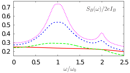
Figure 1: Spectral noise $S_{B}(\omega)/2eI_{B}$ as a function of the normalized frequency $\omega/\omega_{0}$. Different values of the bias are given by: $\omega_{0}=30$ mK (solid red); $\omega_{0}=100$ mK (dashed green); $\omega_{0}=200$ mK (short-dashed blue); $\omega_{0}=300$ mK (dotted magenta). Other parameters are: $\omega_{\mathrm{c}}=5$ K, $\omega_{\mathrm{n}}=50$ mK, $|t_{2}|/|t_{1}|=1$, $T=10$ mK.

V Results

As stated before, for the composite edge states belonging to the Jain sequence, important information about the carrier charges involved in the tunneling can be extracted from the knowledge of the total noise at finite frequency in (11). Each $m$-agglomerate contribution leads to a resonance at $\omega=m\omega_{0}$. This enable us to resolve them and to obtain indications of their power-law behavior. Depending on their scaling dimensions, they show peaks (for $\Delta<1/4$), dips (for $1/4<\Delta<1/2$) or a monotonic increasing as a function of frequency (for $\Delta>1/2$). Note that, for notational convenience, we generically indicated with $\Delta$ both the low energy scaling dimension in (3) and the effective scaling above the neutral mode bandwidth in (4) depending on the considered regime. In figure 1 we show the behavior of the spectral noise for the considered $\nu=2/5$ case at low temperature ($T=10$ mK).

The ratio $S_{B}(\omega)/2eI_{B}$ is plotted in order to recover the proper value of the Fano factor in the zero frequency limit. Ferraro10a ; Carrega12 To further simplify the description, we only focus on the first two contributions to the noise, namely single-qp and $2$-agglomerate, neglecting the contributions due to other possible excitations. Various curves correspond to different values of the applied bias, namely different $\omega_{0}$. Note that in the figure the frequency is rescaled with respect to $\omega_{0}$.

For $\omega_{0}>\omega_{\mathrm{n}}$ (dotted magenta and short-dashed blue curves) it is easy to note a pronounced peak in correspondence of $\omega=\omega_{0}$ due to the single-qp contribution. Despite the fact the temperature is very low, thermal effects leads to a smoothening of the peak. A second contribution, less pronounced, is observable at $\omega=2\omega_{0}$, signature of the presence of the $2$-agglomerate that has a less divergent power-law behavior. This secondary peaks becomes more and more evident by increasing $\omega_{0}$.

For bias voltages such that $\omega_{0}<\omega_{\mathrm{n}}$ (Long-dashed green and solid red curves) the neutral mode contribution increases the scaling dimension turning the single-qp peak into an extremely broad dip that completely hides the $2$-agglomerate contribution. This is a clear demonstration of the fact that the ideal condition to observe the peak patter for the $\nu=2/5$ case is $\omega_{0}>\omega_{\mathrm{n}}$. A remark is in order concerning the role of the temperature. Indeed, the smoothening induced by thermal effects could completely wash away the observed structure under the condition $T>\omega_{\mathrm{n}}$, therefore very low temperature are needed to see this structure.

VI Conclusions

In this paper we analyzed the finite frequency noise for the FQH state at $\nu=2/5$. We considered the presence of the two more relevant excitations: the single-qp, with charge $e/5$, and the $2$-agglomerate, with charge $2e/5$. The finite frequency noise has the unique possibility to resolve spectroscopically the contributions of the different excitations looking at different Josephson resonances. We showed that the peak associated to the $2$-agglomerate is more evident at Josephson frequency higher than the neutral mode cut-off, where the tail of the single-qp contribution decreases faster. We also commented on the evolution of the height of the single-qp peak as a function of temperature, in order to determine the optimal condition for the visibility of the considered peak pattern.

References

References

- (1) Das Sarma S and Pinczuk A 1997 Perspective in quantum Hall effects: novel quantum liquid in low-dimensional semiconductor structures (New York: Wiley)
- (2) Tsui D C 1999 Rev. Mod. Phys. 71 891
- (3) Laughlin R 1983 Phys. Rev. Lett. 50 1395
- (4) Wen X G 1990 Phys. Rev B 41 12838
- (5) Jain J K 1989 Phys. Rev. Lett. 63 199
- (6) Wen X G 1995 Adv. Phys. 44 405
- (7) Wen X G and Zee A 1992 Phys. Rev. B 46 2290
- (8) Chang A M 2003 Rev. Mod. Phys. 75 1449
- (9) de Picciotto R, Reznikov M, Heiblum M, Umansky V, Bunin G and Mahalu D 1997 Nature 389 162
- (10) Saminadayar L, Glattli D C, Jin Y and Etienne B 1997 Phys. Rev. Lett. 79 2526 (1997)
- (11) Reznikov M, de Picciotto R, Griffiths T G, Heiblum M and Umansky V 1999 Nature 399 238
- (12) Chung Y C, Heiblum M and Umansky V 2003 Phys. Rev. Lett. 91 216804
- (13) Bid A, Ofek N, Heiblum M, Umansky V and Mahalu M 2009 Phys. Rev. Lett. 103 236802 (2009)
- (14) Dolev M, Gross Y, Chung Y C, Heiblum M, Umansky V and Mahalu D 2010 Phys. Rev. B. 81 161303(R)
- (15) Ferraro D, Merlo M, Braggio A, Magnoli N and Sassetti M 2008 Phys. Rev. Lett. 101, 166805
- (16) Ferraro D, Braggio A, Magnoli N and Sassetti M 2010 New J. Phys. 12 013012
- (17) Ferraro D, Braggio A, Magnoli N and Sassetti M 2010 Phys. Rev. B 82 085323
- (18) Ferraro D, Braggio A, Magnoli N and Sassetti M 2010 Physica E 42 580
- (19) Carrega M, Ferraro D, Braggio A, Magnoli N and Sassetti M 2011 Phys. Rev. Lett. 107 146404
- (20) Rogovin D and Scalapino D J 1974 Ann. Phys. 86 1
- (21) Zakka-Bajjani E, Segala J, Portier F, Roche P and Glattli D C 2007 Phys. Rev. Lett. 99 236803
- (22) Chamon C, Freed D E and Wen X G 1995 Phys. Rev. B 51 2363
- (23) Chamon C, Freed D E and Wen X G 1996 Phys. Rev. B 53 4033
- (24) Bena C and Nayak C 2006 Phys. Rev. B 73 155335
- (25) Carrega M, Ferraro D, Braggio A, Magnoli N and Sassetti M 2012 New J. Phys. 14 023017
- (26) Levkivskyi I P and Sukhorukov E V 2008 Phys. Rev. B 78 045322
- (27) Levkivskyi I P, Boyarsky A, Frohlich J and Sukhorukov E V 2009 Phys. Rev. B 80 045319
- (28) Kane C L and Fisher M P A 1992 Phys. Rev. Lett. 68 1220
- (29) Rosenow B and Halperin B I 2002 Phys. Rev. Lett. 88 096404
- (30) Papa E and MacDonald A H 2004 Phys. Rev. Lett. 93 126801
- (31) Mandal S S and Jain J K 2002 Phys. Rev. Lett. 89 096801
- (32) Yang K 2003 Phys. Rev. Lett. 91 036802
- (33) Cuniberti G, Sassetti M and Kramer B 1997 J. Phys.: Condens. Matter 8 L21
- (34) Braggio A, Ferraro D, Carrega M, Magnoli N and Sassetti M Preprint arXiv:1203.1906
- (35) Dolcini F, Trauzettel B, Safi I and Grabert H 2005 Phys. Rev. B 71 165309
- (36) Martin T 2005 Les Houches Session LXXXI, ed. Bouchiat et al, (Amsterdam: Elsevier)
- (37) Safi I, Devillard P and Martin T 2001 Phys. Rev. Lett. 86 4628
- (38) Braggio A, Sassetti M and Kramer B 2001 Phys. Rev. Lett. 87 146802
- (39) Cavaliere F, Braggio A, Stockburger J T, Sassetti M and Kramer B 2004 Phys. Rev. B 70 125323
- (40) Cavaliere F, Braggio A, Stockburger J T, Sassetti M and Kramer B 2004 Phys. Rev. Lett. 93 036803
- (41) Gradshteyn I S and Ryzhik I M 1994 Tables of integral, Series, and products (London: Academic Press)