Effect of demographic noise in a phytoplankton-zooplankton model of bloom dynamics

Abstract

An extension of the Truscott-Brindley model (Bull. Math. Biol. 56, 981 (1994)) is derived to account for the effect of demographic fluctuations. In the presence of seasonal forcing, and sufficiently shallow water conditions, the fluctuations induced by the discreteness of the zooplankton component appear sufficient to cause switching between the bloom and no-bloom cycle predicted at the mean-field level by the model. The destabilization persists in the thermodynamic limit of a water basin infinitely extended in the horizontal direction.

I Introduction

Phytoplankton provide the basis of the food chain in the ocean. They are constituted for the large part by microscopic algae and their abundance is such that they are responsible for roughly one half of the total photosynthesis going on in the planet field98 .

Although phytoplankton are present in virtually all of the world hydrosphere (more precisely, the top $100\,$m layer of the water column, called the euphotic layer, where there is enough light for photosynthesis), their distribution in space and time is far from uniform franks97 . Space patchiness is observed at scales that go from that of the individual to several hundreds kilometers blackburn98 ; martin05 . The spatial patterns, revealed e.g. by remote sensing, include filaments, fronts and more irregular shapes, suggesting that turbulent transport by sea currents may play an important role reigada03 ; metcalfe04 ; levy08 ; bracco09 ; mckiver11 .

Variability in time, on the other hand, is characterized by sporadic bloom events in which the plankton density in extended regions can grow by up to three orders of magnitude in few days franks97a . These are seasonal events that may or may not recur annually, and are superimposed onto the weaker day-night and seasonal cycles. Their importance is utmost for several reasons. Depending on the species (e.g. diatoms), due to their abundance, bloom events can have consequences even at the level of the global biogeochemical cycle siegenhalter93 . Bloom events involving other species (e.g. dinoflagellates) can have harmful effects on water quality and fishery smayda97 ; yentsch08 . Being able to predict the onset of algal blooms is clearly an issue of great practical importance.

Several effects of both biological and physical nature contribute to blooms assmy09 . From the point of view of biology, phytoplankton control occurs both top-down (grazing by zooplankton scheffer97 ), and bottom-up (nutrient availability; the microbial loop huppert02 ). In many situations, both mechanisms are expected to contribute simultaneously to the bloom event carbonel99 . Physical processes, such as variation of turbidity in the water basin may03 , modifications in the thermocline smayda97a , and mixing by turbulence huisman99 may equally contribute to the dynamics.

We shall focus in this paper on the particular route to bloom formation provided by failure of the top-down control by zooplankton. Central to this is the so called mismatch issue cushing90 . since the life cycle of phytoplankton is typically one order of magnitude shorter than that of zooplankton, a positive fluctuation in phytoplankton productivity is not compensated by a simultaneous increase in the zooplankton population. This produces the bloom event: the phytoplankton population escapes zooplankton control and grows to the carrying capacity of the medium, before also the zooplankton population grows appreciably, and is able to bring that of the phytoplankton back to its pre-bloom level.

At a sufficiently coarse grained scale, the phytoplankton-zooplankton dynamics can be described by concentration fields $\bar{P}({\bf x},t)$ and $\bar{Z}({\bf x},t)$ evans85 ; truscott94 . This constitutes a mean field approximation for a stochastic individual dynamics; at different levels of complexity, such a description may include the nutrient and even the detritus concentration fields $\bar{N}({\bf x},t)$ and $\bar{D}({\bf x},t)$ (NPZ steele81 ; fasham90 and NPZD edwards01 models). The tininess of both phyto- and zooplankton individuals, as well as the size of typical areas of interest for the study of the concentration dynamics (at least several meters), suggests that a mean field description is indeed the most appropriate. The possibility that bloom events be the outcome of fluctuations in the system, however, should not be discarded. This was the situation observed e.g. in freund06 , in which noise in the external parameters of a compartmental PZ model, was able indeed to produce shifts between bloom and no-bloom cycles.

The noise induced shift between limit cycles in a dynamical system is a well-known effect (see e.g keeling01 for an application to epidemic spreading). In most cases the noise considered is external, but recently there has been a surge of interest in the role of internally generated demographic noise (see e.g. black10 and references therein). The point that we want to examine in the present paper is precisely whether microscopic fluctuations, disregarded in a mean field approach, can resurface at macroscopic scale, generating an internal noise component, sufficient to trigger the bloom event. This is an example of demographic fluctuation induced break-up in the mean field description of reaction-diffusion systems, a type of phenomenon that have received a great deal of attention in recent years young01 ; mckane05 ; doering05 ; butler09 ; butler11 . (Notice that, contrary to e.g. black10 , the noise contribution examined here acts locally in space).

The simple PZ model by Truscott and Brindley (TB model), that is going to be considered here, has the nice characteristic that the plankton behaves like an excitable medium truscott94 . This leads one to expect that noise will be particularly effective in destabilizing its dynamics. (In fact, freund06 considered precisely this model, to generate noise-induced shifts between seasonal bloom and no-bloom cycles). In its original version, the TB model is zero-dimensional, but it can be easily generalized to include spatial effects such as advection and diffusion siekmann08 . In the present analysis, a spatially homogeneous domain will be considered, with no advection, but with diffusive terms accounting for small scale motions in the water column. The game to play will be to determine the demographic fluctuations implicitly neglected in the TB model, and examine under what conditions they can destabilize the system at the level of spatial averages.

This paper is organized as follows. In Sec. II, the main properties of the TB model are reviewed. In Sec. III, the expression for the stochastic contribution to demography are derived. In Sections IV and V, the effect of demographic noise on the dynamics of the TB model, without and with seasonal forcing, is analyzed. Section VI is devoted to the conclusions. Some technical details on the master equation treatment of demographic fluctuations, in spatially extended domains, are provided in the Appendix for reference.

II The Truscott-Brindley model

We review here the main properties of the TB model. For the moment we disregard the spatial structure of the fields and focus on the original zero-dimensional version of the model, which is described by the equations:

$$\dot{\bar{P}} = r_{0}\bar{P}\Big{(}1-\frac{\bar{P}}{K}\Big{)}-R_{m}\frac{\bar{P}^{2}\bar{Z}}{\bar{P}^{2}+\alpha^{2}},$$

$$\dot{\bar{Z}} = -\mu\bar{Z}+\gamma R_{m}\frac{\bar{P}^{2}\bar{Z}}{\bar{P}^{2}+\alpha^{2}}.$$ (1)

The main characteristics of the dynamics are the following:

• Logistic reproductive behavior of the phytoplankton, with the carrying capacity $K$ determining the maximum concentration that the medium can support at steady state.

• Grazing by zooplankton characterized by a so called Holling-III kind of behavior holling59 . Zooplankton are able to graze on phytoplankton with optimal rate $R_{m}\bar{Z}$, only if the concentration of the second is above the level fixed by the half-saturation concentration $\alpha$. Below this threshold, the grazing rate is quadratic in $\bar{P}$: $R_{m}(\bar{P}/\alpha)^{2}\bar{Z}$, reflecting both a reduced grazing ability of the zooplankton in a dilute environment, and the actual reduced amount of food available.

• A carrying capacity of the medium supposed much larger than the half saturation concentration, $K\gg\alpha$, meaning that at high values of $\bar{P}$, the ability of zooplankton to control phytoplankton growth is limited.

• A zooplankton reproductive dynamics supposed slower than that of the phytoplankton: $\mu/R_{m}\ll 1$, while $r_{0}/R_{m}\sim 1$. A conversion efficiency $\gamma$ assumed consistently small.

The default values of the constants that are utilized in the zero-dimensional case are truscott94 :

$$r_{0}=0.3/{\rm day},\quad R_{m}=0.7/{\rm day},\quad\mu=0.012/{\rm day},$$

$$K=108{\rm mg\,C/m^{3}},\quad\alpha=5.7{\rm mg\,C/m^{3}},$$ (2)

$$\gamma=0.05,$$

where the units “${\rm mg\,C}$” stand for carbon milligrams in dry weight. From here we can extract three independent dimensionless groups

$$\hat{r}_{0}=\frac{r_{0}}{R_{m}}\simeq 0.43,\quad q=\frac{\mu}{\gamma R_{m}}\simeq 0.34,$$

$$\epsilon=\frac{\alpha}{K}\simeq 0.053.$$ (3)

We see that the dynamics is characterized by two independent small parameters: $\gamma$ and $\epsilon$. The dynamics described by Eq. (1) has a fixed point at the scale of the half-saturation constant $\alpha$:

$$P_{f} = \alpha\sqrt{\frac{q}{1-q}},$$

$$Z_{f} = \frac{\hat{r}_{0}}{P_{f}}(1-\frac{P_{f}}{K})(\alpha^{2}+P_{f}^{2})\simeq\frac{\alpha\hat{r}_{0}}{\sqrt{q(1-q)}}.$$ (4)

For small $\gamma,\epsilon\ll 1$ and $q<1/2$, this fixed point is globally attracting (a Holling-III functional form for grazing appears to be crucial for stability). However, if the initial zooplankton concentration is too low, before reaching the fixed point, the system will make an excursion to the high $\bar{P}\sim K$ range, which could be interpreted as a bloom event. The situation is illustrated in Fig. 1. As shown in figure, the onset of bloom could roughly be identified in the $\bar{P}\bar{Z}$ plane by the line where the largest eigenvalue of the Jacobian of Eq. (1) crosses to positive, and phase points start to separate exponentially.

Figure 1: Trajectories approaching the fixed point $(P_{f},Z_{f})$ (fat dot to lower left corner of picture) starting from different initial conditions; going from outer to inner trajectory: $(\bar{P},\bar{Z})=(0.5,0.5);\ (0.5.0.6);\ (0.6,0.66);\ (0.6,0.68)$. The parameters are those of Eq. (2). The dotted line indicate change of signature of the Jacobian matrix for Eq. (1), and could roughly be identified as the point where the bloom begins.

The above picture of bloom triggering by zooplankton depletion can be improved including the effect of seasonal forcing. Model equations (1) can accommodate this effect by letting the phytoplankton productivity $r$ become dependent on the temperature, as suggested in freund06 . The parameterization that we adopt is the same as in freund06 : a Van’t Hoff kind of dependence for $r$ berges02 :

$$r_{0}\to r(T)=r_{0}\ 2^{\upsilon(T-T_{0})}$$ (5)

and a sinusoidal dependence on time of the temperature:

$$T(t)=T_{0}+\Delta T\sin(\Omega t+\phi).$$ (6)

with $\Omega=2\pi/(365\ {\rm days})$ to allow for an annual cycle, and $\phi/(2\pi)=0.59$, to have that setting $t=0$ on January 1st, causes the first temperature minimum to occur on March 1st and the first maximum on August 29th. For the sake of definiteness, as in freund06 , we set $\Delta T=6{\rm{}^{o}C}$ and $\upsilon=0.1\,{\rm{}^{o}C}^{-1}$.

Adding a seasonal forcing, turns out to modify the dynamics in important way, with the single fixed point in the autonomous case leaving way to two stable limit cycles freund06 . The situation is illustrated in Fig. 2: a small amplitude no-bloom cycle coexists with a large amplitude bloom cycle, each one characterized by a well defined (time-dependent) basin of attraction.

Figure 2: Bloom and no-bloom cycles (heavy and thin lines respectively) in the seasonally forced TB model. The phase points circle counterclockwise along the cycle. Notice that the intersections of the two cycles corresponds to phese points that in the two cycles are associated to different (although close) instants of time. The dotted vertical line gives the position of the fixed points that would correspond to the different values taken by $\hat{r}$ during the year. The fat dot still identifies the fixed point corresponding to $\hat{r}=\hat{r}_{0}$. The parameters in the graph are those in Eqs. (5-6).

As illustrated in Fig. 3, the small cycle will remain stable only if the seasonal temperature excursion $\Delta T$ is below a critical threshold $\Delta T_{crit}(\hat{r}_{0},q,\epsilon,\gamma)$, that, for the values of the parameters quoted in Eqs. (2) is $\Delta T_{crit}\simeq 6.1{\rm{}^{o}C}$.

Figure 3: Dependence on the critical forcing amplitude $\Delta T_{crit}$ on the parameters $\gamma$ (thin line), $\epsilon$ (heavy line) and $q$ (insert). In the three cases $\Delta T_{\gamma,\epsilon,q}$ indicate the value of $\Delta T_{crit}$ obtained varying $\gamma,\epsilon,q$ respectively and keeping the remaining parameters fixed to the values in Eq. (3).

Similarly, it can be shown that, if $\Delta T$ is too small, only the no-bloom cycle will survive. The no-bloom destabilization threshold is very close to the value of the forcing $\Delta T=6{\rm{}^{o}C}$ considered in freund06 . The analysis in that paper showed in fact that addition of a fluctuating component to the forcing, lead to random switch from year to year between the two regimes. As it is clear from Fig. 2, the destabilization is likely to take place near the intersection between the bloom and no-bloom trajectories, where the separation between the phase points of the two cycles (at equal times) is smaller.

III Demographic fluctuations

We consider a situation in which the typical size of a zooplankton individual is much larger than that of a typical phytoplankter. A reasonable estimate (with large variations) for the mass of a copepod could be, for instance:

$$m_{Z}\sim 20{\rm\mu g\,C},$$ (7)

corresponding to a typical individual size in the millimeter range gonzalez08 ; metcalfe04 . In a no-bloom regime $\bar{P},\bar{Z}\sim\alpha$ with $\alpha$ given as in Eq. (2), Eq. (7) would lead to a numerical density of the order of one zooplankton individual per liter. Given the much smaller size of microscopic algae, phytoplankton could in turn be treated as a continuum at those scales. We thus expect that the demographic fluctuations in the system be driven by the zooplankton.

Locally, demographic fluctuations will be the result of a competition between stochasticity at the individual level of the birth-death process, and mixing by spatial transport. We shall consider a two-dimensional situation, in which the vertical structure of the water column is not resolved, and parameterize horizontal mixing through a diffusivity $\kappa$, supposed equal for both phyto- and zooplankton. This is probably the only viable strategy to describe a very complex situation, in which microscopic swimming, stirring by larger organisms, turbulence generated by perturbations at the water surface, all play an important role note . Likewise, we shall neglect all effects of large scale advection, including the forcing induced by the formation of fronts, where the two plankton populations may get out of balance reigada03 .

Including the possibility of a 2D spatial structure, the original model equations (1) can be written in the form

$$\dot{\bar{P}} = B_{P}(\bar{P},\bar{Z})-D_{P}(\bar{P},\bar{Z})+\kappa\nabla^{2}\bar{P},$$

$$\dot{\bar{Z}} = B_{Z}(\bar{P},\bar{Z})-D_{Z}(\bar{P},\bar{Z})+\kappa\nabla^{2}\bar{Z},$$ (8)

where $B_{PZ}$ and $D_{PZ}$ give the local birth and death rates in the population, and $\bar{P}=\bar{P}({\bf x},t)$ and $\bar{Z}=\bar{Z}({\bf x},t)$ give the plankton concentration averaged over the height of the water column. Expressing time in units $R_{m}^{-1}$ and concentrations in units $\alpha$ (and lengths in terms of some reference scale), the parameters entering Eq. (8) can be written in the form

$$B_{P}=\hat{r}\bar{P};\qquad D_{P}=\epsilon\hat{r}\bar{P}^{2}+\bar{P}^{2}\bar{Z}/(1+\bar{P}^{2});$$

$$B_{Z}=\gamma\bar{P}^{2}\bar{Z}/(1+\bar{P}^{2});\qquad D_{Z}=\gamma q\bar{Z}.$$ (9)

From now on, unless otherwise stated, all relations will be expressed in dimensionless form.

Rather than working in a field theoretical setting doi76 , we prefer to apply the standard system size expansion approach of van Kampen directly to the master equation for the system vankampen . Let us therefore partition the domain in volumes of horizontal size $\Delta x$, each one containing instantaneously $N_{P},N_{Z}$ individuals of the $P$ and $Z$ groups. We can introduce instantaneous concentrations $P,Z=\Omega_{P,Z}^{-1}N_{P,Z}$, coarse grained at horizontal scale $\Delta x$, with

$$\Omega_{P,Z}=h(\Delta x)^{2}/m_{P,Z}$$ (10)

parameterizing the size of the population in the volumes, and $h$ indicating the height of the water column. Indicate with $\tilde{P}=P-\bar{P}$ and $\tilde{Z}=Z-\bar{Z}$ the fluctuating part of the coarse-grained field; in the present situation of fluctuations driven by zooplankton discreteness, we expect $\tilde{P}/\bar{P},\tilde{Z}/\bar{Z}=O(N_{Z}^{-1/2})$. Let us define normalized fluctuation fields $\phi,\zeta$ with this scaling contribution factored out:

$$N_{P} = \Omega_{P}P:=\Omega_{P}(\bar{P}+\Omega_{Z}^{-1/2}\phi),$$

$$N_{Z} = \Omega_{Z}Z:=\Omega_{Z}(\bar{Z}+\Omega_{Z}^{-1/2}\zeta).$$

Following the strategy utilized in butler09 ; butler11 ; bonachela12 , we adopt as modelling assumption that the birth and death rates $B_{P,Z}$ and $D_{P,Z}$ at the population scale, reflect birth and death rates at the individual level, conditioned to the instantaneous values of the concentration fields $P({\bf x},t)$ and $Z({\bf x},t)$. An hypothesis of independence and Markovianity of the birth-death events, at scales of interest, underlies this assumption. At the population level, the transition probabilities ${\rm d}\mathcal{P}$ in an interval ${\rm d}t$ will be therefore:

$$N_{P}\to N_{P}+1: {\rm d}\mathcal{P}=\Omega_{P}B_{P}(P,Z){\rm d}t,$$ (11)

$$N_{P}\to N_{P}-1: {\rm d}\mathcal{P}=\Omega_{P}D_{P}(P,Z){\rm d}t,$$

$$N_{Z}\to N_{Z}+1: {\rm d}\mathcal{P}=\Omega_{Z}B_{Z}(P,Z){\rm d}t,$$

$$N_{Z}\to N_{Z}-1: {\rm d}\mathcal{P}=\Omega_{Z}D_{Z}(P,Z){\rm d}t,$$

and $B_{P}/P,\ldots D_{Z}/Z$ will be the corresponding birth and death probabilities per unit time for the individuals.

A standard procedure vankampen leads, from Eq. (11), to the master equation for the probability density function (PDF) $\rho(\{\phi_{i},\zeta_{i}\},t)$ (the index $i$ labels the volumes in the domain):

$$\frac{\partial\rho}{\partial t} = \sum_{i}\left\{\Pi_{i}\rho+\Omega_{Z}^{1/2}\Big{[}\dot{\bar{P}}_{i}\frac{\partial\rho}{\partial\phi_{i}}+\dot{\bar{Z}}_{i}\frac{\partial\rho}{\partial\zeta_{i}}\Big{]}\right.$$ (12)

$$+ \Omega_{P}\Big{\{}\Big{[}\exp\Big{(}-\Omega_{C}^{-1/2}\frac{\partial}{\partial\phi_{i}}\Big{)}-1\Big{]}B_{P,i}$$

$$+ \Big{[}\exp\Big{(}\Omega_{C}^{-1/2}\frac{\partial}{\partial\phi_{i}}\Big{)}-1\Big{]}D_{P,i}\Big{\}}\rho$$

$$+ \Omega_{Z}\Big{\{}\Big{[}\exp\Big{(}-\Omega_{Z}^{-1/2}\frac{\partial}{\partial\zeta_{i}}\Big{)}-1\Big{]}B_{Z,i}$$

$$+ \left.\Big{[}\exp\Big{(}\Omega_{Z}^{-1/2}\frac{\partial}{\partial\zeta_{i}}\Big{)}-1\Big{]}D_{Z,i}\Big{\}}\rho\right\},$$

where $\Omega_{C}^{1/2}=\Omega_{Z}^{-1/2}\Omega_{P}$, and the additional term $\Pi_{i}\rho$ accounts for the exchange of plankton between adjacent volumes produced by diffusion (see Appendix). Expanding to lowest order in $\Omega_{P,Z}^{-1}$, both the exponentials and the reaction rates in Eq. (12) [recall that $B_{P}=B_{P}(\bar{P}+\Omega^{-1/2}_{Z}\phi,\bar{Z}+\Omega^{-1/2}_{Z}\zeta),\ldots$], we obtain the Fokker-Planck equation:

$$\frac{\partial\rho}{\partial t} + \sum_{i}\Big{\{}\frac{\partial}{\partial\phi_{i}}\Big{(}a_{{\scriptscriptstyle{PP}},i}\phi_{i}+a_{{\scriptscriptstyle{PZ}},i}\zeta_{i}\Big{)}\rho$$ (13)

$$+ \frac{\partial}{\partial\zeta_{i}}\Big{(}a_{{\scriptscriptstyle{ZP}},i}\phi_{i}+a_{{\scriptscriptstyle{ZZ}},i}\zeta_{i}\Big{)}\rho\Big{\}}$$

$$= \sum_{i}\Pi_{i}\rho+\frac{1}{2}\sum_{ij}\frac{\partial}{\partial\zeta_{i}}\frac{\partial}{\partial\zeta_{j}}\Xi_{ij}\rho,$$

where $\Xi_{ij}=[B_{Z}(\bar{P}_{i},\bar{Z}_{i})+D_{Z}(\bar{P}_{i},\bar{Z}_{i})]\delta_{ij}$, and the $a_{\scriptscriptstyle{PP}},\ldots$ give the entries of the Jacobian matrix for Eq. (1) ($a_{\scriptscriptstyle{PP}}\equiv\partial\dot{\bar{P}}/\partial\bar{P},\ldots$). Notice that the only noise correlator present in the equation, $\Xi_{ij}$, is the one associated with the variable $\zeta$, i.e. with the zooplankton fluctuations.

The dependence of the expansion parameter $\Omega_{Z}^{-1}$ on the arbitrary coarse graining scale $\Delta x$ may look somewhat confusing, as different $\Delta x$ correspond to different fluctuation levels at the coarse-graining scale. We see in particular that $\Omega_{Z}$ goes to zero with $\Delta x$. Nevertheless, as it will become clear in the next section, there exists a natural microscopic scale $\lambda_{c}$ below which fluctuations are smeared out by diffusion. Thus, applicability of the system size expansion rests on smallness of fluctuations at scale $\lambda_{c}$, and not on the choice of $\Delta x$.

Going back to the original variables $\tilde{P},\tilde{Z}$, and taking the continuous limit, we see that the Fokker-Planck equation (13) is equivalent to the system of Langevin equations

$$\frac{\partial\tilde{P}}{\partial t}+a_{\scriptscriptstyle{PP}}\tilde{P}+a_{\scriptscriptstyle{PZ}}\tilde{Z}=\kappa\nabla^{2}\tilde{P}$$

$$\frac{\partial\tilde{Z}}{\partial t}+a_{\scriptscriptstyle{ZP}}\tilde{P}+a_{\scriptscriptstyle{ZZ}}\tilde{Z}=\kappa\nabla^{2}\tilde{Z}+\xi,$$ (14)

where

$$\langle\xi({\bf x},t)\xi({\bf x}^{\prime},0)\rangle=\Xi({\bf x},t)\delta({\bf x}-{\bf x}^{\prime})\delta(t),$$

$$\Xi({\bf x},t)=\hat{m}_{Z}[B_{Z}(\bar{P},\bar{Z})+D_{Z}(\bar{P},\bar{Z})],$$ (15)

and we have put $\hat{m}_{Z}=m_{Z}/h$, $\bar{P}\equiv\bar{P}({\bf x},t)$ and $\bar{Z}\equiv\bar{Z}({\bf x},t)$ (more details in the Appendix).

IV Dynamics near the fixed point

Let us consider first the case of a TB model without seasonal forcing, and study the fluctuations around the fixed point given by Eq. (4). The analysis is similar to the one carried on in butler11 on another PZ model (the Levin-Segel model levin76 ), which focused on the destabilization of Turing patterns (see also biancalani11 for another example of Turing pattern destabilization a reaction-difusion system). The calculation will allow to identify the relevant fluctuation scales on which to base the forced case analysis in the next section.

The evolution equations for the correlation functions $C_{PP}({\bf x},t)=\langle\tilde{P}({\bf x},t)\tilde{P}(0,t)\rangle,\ldots$ can be obtained from Eqs. (14-15), and take the form in Fourier space:

$$\frac{1}{2}\dot{C}_{PP{\bf k}}+(a_{\scriptscriptstyle{PP}}+\kappa k^{2})C_{PP{\bf k}}+a_{\scriptscriptstyle{PZ}}C_{PZ{\bf k}}=0$$

$$\dot{C}_{PZ{\bf k}}+a_{\scriptscriptstyle{ZP}}C_{PP{\bf k}}+(a_{\scriptscriptstyle{PP}}+a_{\scriptscriptstyle{ZZ}}+2\kappa k^{2})C_{PZ{\bf k}}$$

$$\qquad\;\;\;+a_{\scriptscriptstyle{PZ}}C_{ZZ{\bf k}}=0$$

$$\frac{1}{2}\dot{C}_{ZZ{\bf k}}+a_{\scriptscriptstyle{ZP}}C_{PZ{\bf k}}+(a_{\scriptscriptstyle{ZZ}}+\kappa k^{2})C_{ZZ{\bf k}}=\Xi.$$ (16)

At the fixed point we find immediately, using Eq. (9) and working to lowest order in $\epsilon$ and $\gamma$:

$$a_{\scriptscriptstyle{PP}}\simeq-\hat{r}(1-2q),\quad a_{\scriptscriptstyle{PZ}}=-q,$$

$$a_{\scriptscriptstyle{ZP}}\simeq 2\gamma\hat{r}(1-q),\quad a_{\scriptscriptstyle{ZZ}}=0,$$

$$\Xi\simeq 2\gamma\hat{m}_{Z}\sqrt{q/(1-q)}.$$ (17)

Equation (16) becomes at steady state:

$$(a_{\scriptscriptstyle{PP}}+\kappa k^{2})C_{PP{\bf k}}+a_{\scriptscriptstyle{PZ}}C_{PZ{\bf k}}=0,$$

$$a_{\scriptscriptstyle{ZP}}C_{PP{\bf k}}+(a_{\scriptscriptstyle{PP}}+2\kappa k^{2})C_{PZ{\bf k}}+a_{\scriptscriptstyle{PZ}}C_{ZZ{\bf k}}=0,$$

$$a_{\scriptscriptstyle{ZP}}C_{PZ{\bf k}}+\kappa k^{2}C_{ZZ{\bf k}}=\Xi,$$

that has solution

$$C_{PP{\bf k}} \simeq \Delta^{-1}a_{\scriptscriptstyle{PZ}}^{2}\Xi,$$

$$C_{PZ{\bf k}} \simeq \Delta^{-1}a_{\scriptscriptstyle{PZ}}(-a_{\scriptscriptstyle{PP}}+\kappa k^{2})\Xi,$$

$$C_{ZZ{\bf k}} \simeq \Delta^{-1}(-a_{\scriptscriptstyle{PP}}+\kappa k^{2})^{2}\Xi,$$ (18)

with

$$\Delta=a_{\scriptscriptstyle{PP}}a_{\scriptscriptstyle{PZ}}a_{\scriptscriptstyle{ZP}}+a_{\scriptscriptstyle{PP}}^{2}\kappa k^{2}-2a_{\scriptscriptstyle{PP}}\kappa^{2}k^{4}+\kappa^{3}k^{6}.$$ (19)

From Eqs. (18-19), we see that there is a long wavelength range, dominated by demography; using Eq. (17):

$$C_{PP{\bf k}} \simeq \frac{q\hat{m}_{Z}}{\hat{r}_{0}^{2}(1-q)(1-2q)}\sqrt{\frac{q}{1-q}},$$

$$C_{PZ{\bf k}} \simeq \frac{\hat{m}_{Z}}{\hat{r}_{0}(1-q)}\sqrt{\frac{q}{1-q}},$$

$$C_{ZZ{\bf k}} \simeq \frac{\hat{m}_{Z}(1-2q)}{q(1-q)}\sqrt{\frac{q}{1-q}}.$$ (20)

At small scales, the fluctuations are smeared out by diffusion, with the asymptotic law $C_{PP{\bf k}}\simeq a_{\scriptscriptstyle{PP}}^{2}\Xi/(\kappa k^{2})^{3}$, $C_{PZ{\bf k}}\simeq a_{\scriptscriptstyle{PZ}}\Xi/(\kappa k^{2})^{2}$, $C_{PZ{\bf k}}\simeq\Xi/(\kappa k^{2})$. The transition occurs at $\kappa k^{2}\sim a_{\scriptscriptstyle{ZP}}a_{\scriptscriptstyle{PZ}}/a_{\scriptscriptstyle{PP}}$, which sets the crossover length, from Eqs. (3) and (17), back to dimensional units:

$$\lambda_{c}=\sqrt{\kappa/\mu}.$$ (21)

This is the typical distance travelled by a zooplankter in a lifetime and corresponds to the characteristic wavelength of the chemical waves supported by the system in the mean field. Notice that, contrary to the case considered in siekmann08 , for the choice of parameters utilized, no Turing instability is present.

The correlation spectrum that has been obtained, characterized by a plateau at $k\lambda_{c}<1$, and a decay at $k\lambda_{c}>1$, corresponds to fluctuations with a correlation scale $\lambda_{c}$. The fluctuation amplitude can be estimated approximating the decay at $k\lambda_{c}>1$ with a step function and approximating the solution for $k\lambda_{c}<1$ with Eq. (20). This gives for the fluctuation amplitude

$$C_{PP}(0)=\mathcal{F}^{-1}_{{\bf x}=0}[C_{PP{\bf k}}]\sim\lambda_{c}^{-2}C_{PP0},$$

with $C_{PP0}$ as given in Eq. (20), and similar expressions for $C_{PZ}(0)$ and $C_{ZZ}(0)$. From Eqs. (20) we get for the ratio of the fluctuation amplitude to the mean (back to dimensional units):

$$\frac{C_{PP}(0)}{\bar{P}^{2}}\sim\frac{C_{PZ}(0)}{\bar{P}\bar{Z}}\sim\frac{C_{ZZ}(0)}{\bar{Z}^{2}}\sim\frac{m_{Z}}{\alpha h\lambda_{c}^{2}},$$ (22)

that is the ratio of the zooplankter mass and the typical total zooplankton mass in a water column of height $h$ and horizontal extension $\lambda_{c}$.

V Destabilization of the no-bloom regime

Let us pass to consider a seasonally forced situation and ask under what conditions, demographic noise could destabilize global bloom and no-bloom cycles.

Clearly, the linearized theory of Sec. IV cannot be utilized in the present case, as the trajectories evolve for most of their time in an unstable region, as depicted in Fig. 1. A first possibility is at this point numerical solution of the master equation (12) by Montecarlo techniques, utilizing the transition probabilities in Eq. (11) to deal with the birth and death events in the computational cells $\Delta x$, and the transfer rates $W_{i}$ introduced in Appendix A to deal with diffusion. In alternative, the Langevin equation (14) can be integrated numerically, after replacement of the Jacobian matrix $a_{ij}$ with the full RHS (right hand side) of Eq. (8), to extend beyond linear regime the region of validity of the equation

It is convenient to express lengths in units $\lambda_{c}$, so that the forced equation can be written in the form

$$\dot{P} = B_{P}(P,Z)-D_{P}(P,Z)+\gamma q\nabla^{2}P,$$

$$\dot{Z} = B_{Z}(P,Z)-D_{Z}(P,Z)+\gamma q\nabla^{2}Z+\xi.$$ (23)

Notice the dependence of the terms on RHS of Eq. (23) on the fluctuating fields $P$ and $Z$; similarly, the dependence on $\bar{P}$ and $\bar{Z}$ in Eq. (15) is replaced by one on $P$ and $Z$:

$$\langle\xi({\bf x},t)\xi({\bf x}^{\prime},0)\rangle=\Xi({\bf x},t)\delta({\bf x}-{\bf x}^{\prime})\delta(t),$$

$$\Xi({\bf x},t)=\hat{m}_{Z}[B_{Z}(P,Z)+D_{Z}(P,Z)].$$ (24)

The parameter $\hat{m}_{Z}$, which, through Eq. (24), determines the amplitude of the noise $\xi$, takes the form, in terms of dimensional parameters:

$$\hat{m}_{Z}=\frac{m_{Z}\mu}{\alpha h\kappa}.$$ (25)

This quantity will play the role of a control parameter for the theory. [We notice by the way that $\hat{m}_{Z}$ coincides with the amplitude ratio in Eq. (22)].

The results that follow come from direct numerical simulation of Eqs. (23-24) in a periodic domain using a simple finite difference scheme (centered in space, forward Euler in time). Except for very large values of $\hat{m}_{Z}$, the results can be shown to coincide with those of Montecarlo simulation montecarlo . (For larger values of $\hat{m}_{Z}$, the discretization $\Delta x<\lambda_{c}$ would become small enough for local extinction in the computation cells $\Delta x$ to become a problem, and either Montecarlo, or more sophisticated algorithms, such as those described in dornic05 ; moro04 , should be utilized).

As expected, a sufficiently high level of noise destabilizes the small cycle and leads to locking the system in the large bloom cycle. As illustrated in Fig. 4, the threshold in $\hat{m}_{Z}$ becomes lower as the critical forcing $\Delta T_{crit}$ is approached.

Figure 4: No-bloom cycle destabilization threshold in function of $\Delta T$, from numerical simulation in a periodic domain $200\Delta x\times 200\Delta x$ with $\Delta x=\lambda_{c}/10$. The no-bloom cycle is considered destabilized if the system crosses the threshold $\bar{P}=10$ before $t=10\,$years. All parameters except $\Delta T$ and $\hat{m}_{Z}$ set to the values in Eqs. (2) and (7). Initial conditions set equal to $(P_{f},Z_{f})$ uniformly in the domain.

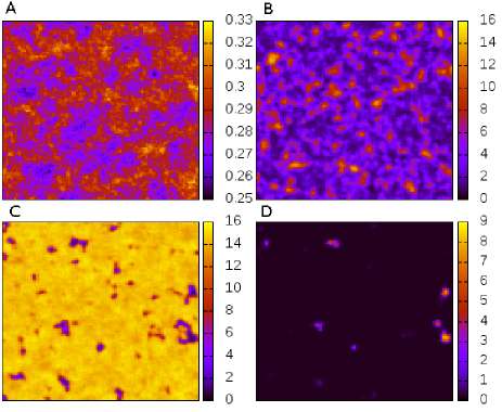
Figure 5: (Color online). Snapshots of the phytoplankton concentration field from a simulation with $\hat{m}_{Z}=10^{-4}$; $\Delta T=6\,{\rm{}^{o}C}$ and other parameters set as in Eqs. (2) and (7). Size of the domain $200\Delta x\times 200\Delta x$; periodic boundary conditions, with $\Delta x=0.3\lambda_{c}$. Initial conditions set equal to $(P_{f},Z_{f})$ uniformly in the domain. A: day 700 (December 1st: no-bloom condition); B: day 890 (May 9th: pre-bloom condition); C: day 924 (June 13th: bloom peak); D: day 970 (July 29: concentration minimum after bloom).

Figure 6: (Color online). Same as Fig. 5 in the case of the zooplankton field.

Figure 7: Top figure: evolution of the mean concentration fields $\bar{P}$ (thin line) and $\bar{Z}$ (heavy line). Bottom figure: evolution of the normalized RMS fluctuations $\hat{\sigma}_{P}=\langle\tilde{P}^{2}\rangle^{1/2}/\bar{P}$ (thin line), $\hat{\sigma}_{Z}=\langle\tilde{Z}^{2}\rangle^{1/2}/\bar{Z}$ (heavy line), $\hat{c}_{PZ}={\rm sign}(\langle\tilde{P}\tilde{Z}\rangle)|\langle\tilde{P}\tilde{Z}\rangle/(\bar{P}\bar{Z})|^{1/2}$ (dotted line). Same choice of parameters as in Figs. 5 and 6.

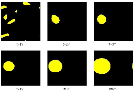
Figure 8: (Color online). Evolution due to the effect of diffusion, in the absence of noise, of domains characterized by bloom dynamics (light gray in figure – yellow on web; a bloom event at a given pixel is identified by crossing during the year of the threshold $P=12$). The initial condition at $t=0$ was a random distribution in space of values $P,Z$ in the bloom and no-bloom basin of attraction. Initial fraction of bloom points: 0.235 (for larger fractions, the system locks immediately on a bloom-cycle; the opposite for lower fractions). Domain characteristics and parameters as in Figs. 5-6.

For default values of the parameters, such as those in Eqs. (2) and (7), with $\Delta T=6{\rm{}^{o}C}$, the threshold would be at $\hat{m}_{Z}\simeq 4\cdot 10^{-5}$, which, for a depth $h\simeq 5\,{\rm m}$, would correspond to a diffusivity $\kappa\simeq 0.2\,{\rm m^{2}/day}\equiv 0.024{\rm cm^{2}/s}$ and a correlation length $\lambda_{c}\simeq 4.1{\rm m}$. In comparison, $\kappa\sim 0.01\,{\rm cm^{2}/s}$ would be the diffusivity that would be produced by microscopic swimming at speed $\sim 1\,{\rm mm/s}$ with a persistence time between change of directions of the order of one second metcalfe04 .

As illustrated in Fig. 5, even when the system is locked globally on a bloom cycle, its dynamics is characterized by spatial fluctuations, with regions of size $\sim\lambda_{c}$ in which, during bloom events, $P$ remains well below its typical bloom value.

This picture is confirmed by looking at the evolution of the RMS fluctuations, as depicted in Fig. 7. The stronger fluctuation level in the phytoplankton concentration field, at the onset of the bloom events and soon after their disappearance, that can be seen in case $B$ and $D$ in Fig. 5, is paralleled by the double peaks in $\hat{\sigma}_{P}$ in Fig. 7.

The above picture of global destabilization of the no-bloom cycle is based on numerical evidence from simulations in a finite domain. One may question whether destabilization could be just a finite size effect, and would disappear in the thermodynamic limit. One suggestion that this is not the case comes from the invasive character of the destabilization phenomenon. The sequence $B-C$ in Fig. 5 gives a hint of the process: regions of size $\sim\lambda_{c}$, characterized by high values of $P$, through diffusive coupling, destabilize nearby regions with low values of $P$, and push them into the bloom cycle. This picture is corroborated by the behavior of the system in the noiseless $\hat{m}_{Z}=0$ case. As shown in Fig. 8, in the absence of noise, the phenomenon persists: phytoplankton transfer across a $\sim\lambda_{c}$ distance, from a bloom to a no-bloom region, destabilizes the second one. Thus, if a bloom bubble is sufficiently large (on the scale of $\lambda_{c}$), it will survive diffusive transfer and gradually expand at the expenses of the surroundings. It is possible to see that the situation is confirmed in the case of a system with just two homogeneous compartmens coupled diffusively, one evolving on a bloom cycle, the other on a no-bloom cycle: the no-bloom cycle will always be destabilized and the system will lock on a global bloom cycle.

This suggests the following picture:

• Demographic noise continuously generates local fluctuations in $P$ and $Z$ (especially in $Z$) that may push some regions of space in a bloom regime.

• If the noise level is sufficiently high, some of these regions will be large enough for not being destroyed at once by diffusivity (see passage from year 1 to year 2 in Fig. 8).

• At this point diffusion, through phytoplankton transfer, quickly destabilizes the surrounding no-bloom regions. Noise is not expected to be important any more in this phase.

VI Conclusions

The TB model, both in its zero-dimensional version, and in the extended one describing the evolution of $P$ and $Z$ fields, can be seen as a mean field description of some individual level model (ILM). The most natural way to obtain an individual dynamics from a global one, is to assume that the birth and death rates at the individual level have the same form as the corresponding quantities at the population level. Within these assumptions, independence of the birth and death events, together with absence of memory effects at the scales of interest, fix the form of the ILM. A master equation describing its dynamics can thus be obtained, utilizing techniques analogous to those in butler09 ; butler11 .

It should be stressed that this is only one of the ways in which an ILM could be obtained from a population level model. Any choice, differing from the present one by identical contributions in the individual birth and death rates, would work as well, as the equations at the population level would remain unchanged. The issue is particularly important for the zooplankton, that is the source of fluctuations for the model. Nevertheless, the zooplankton death rate $\mu$ appearing the population level equation (1) already reflect modelling assumptions at the individual level, so that the present choice of ILM is somewhat imposed.

Keeping in mind all these caveats, analysis of the results from the ILM shows that, for shallow water conditions (few meters depth), and mixing in the water column produced by diffusion (diffusivity in the range $0.1\,{\rm m^{2}/day}$), demographic noise is sufficient to cause switching between regimes. The effect is of the same order of magnitude as that of the global temperature fluctuations considered in freund06 (fluctuation amplitude $\sim 1\,{\rm{}^{o}C}$ with correlation time equal to 35 days). From the point of view of the PZ model, this corresponds to a decrease of the instability threshold in the seasonal temperature forcing, with respect to the mean-field case, of the order of $1\,{\rm{}^{o}C}$ (see Fig. 4).

An interesting aspect of the present analysis, common to what was obtained in butler11 in the case of Turing waves, is how local fluctuations are able to produce a global destabilization in the system, that is expected to be maintained in the thermodynamic limit of an infinite basin. The reason is partly trivial: the reproduction rates at the population level are nonlinear functions of the concentration fields $P$ and $Z$, and fluctuations lead necessarily to their renormalization. Such a picture, however, is incomplete, as the destabilization process, in the present case, unless the demographic noise is very large, destabilizes the system only locally. (The characteristic scale of the fluctuations coincides with that of the Turing patterns of the system, and has nothing to do with stochastic demography). Only later, by an invasive process, which appears to be insensitive to system size, the destabilized regions rapidly inglobate the inactive surroundings, leading to the global bloom cycle.

It is interesting to notice that, as illustrated in Fig. 5, the invasive dynamics is associated with a spatially intermittency of the $P$ field in the pre-bloom phase, with the high $P$ regions acting as seeds for the coming bloom phase. This condition could be utilized in experiments to contrast the particular destabilization mechanism described here, with the one provided, say, by global temperature fluctuations.

Again as regards the spatial structure of the blooms, it is worth comparing the role of the characteristic length $\lambda_{c}$ defined in Eq. (21), with the vertical inhomogeneity scales considered in huisman99 . In both cases, the bloom event is produced by a local phytoplankton growth that is not balanced by dispersion. In one case, horizontally, in the other, in the vertical direction. The present model bypassed all difficulties associated with the vertical plankton distribution and vertical structure of the water basin, considering implicitly a shallow water condition. An interesting question is therefore, whether phenomena such as the “critical turbulence” in huisman99 may act as a localization mechanisms, that lets the destabilization route described in this paper act also in deep water.

A different question concerns the robustness of the present results under extension of the model to inclusion of bottom-up effects by nutrients from one side, or inclusion of finer grained details in the PZ dynamics. While one would expect irrelevance of the $Z$ fluctuations in a nutrient unbalance dominated bloom scenario, such as the one depicted in huppert02 , the question remains open as regards the situation in which zooplankton control is dominant. The feedback by an increase of the zooplankton deaths, on the nutrient field, and then on the phytoplankton growth rate [the parameter $r_{0}$ in Eq. (1)], would suggest a positive effect. Closer scrutiny is clearly required.

Appendix A Master equation treatment of diffusion

We consider for simplicity a one-dimensional domain and a single species, say $Z$. Discretize the domain and indicate with $N_{i}$ the number of individuals in slot $i$. We can define the PDF’s:

$$\rho_{\bf N}({\bf N}) \equiv \rho_{\bf N}(\{\Omega\bar{Z}_{i}+\Omega^{1/2}\zeta_{i},i=1,\ldots K\})$$

$$= \Omega^{-K/2}\rho_{\boldsymbol{\zeta}}({\boldsymbol{\zeta}}).$$

Suppose that individuals are transferred diffusively from slot $i$ to slot $i\pm 1$ with a rate $W_{i\to i+1}=W_{i\to i-1}\equiv W_{i}=N_{i}\hat{\kappa}_{i}$, where $\hat{\kappa}_{i}=\kappa_{i}/(\Delta x)^{2}$, with $\kappa_{i}\equiv\kappa({\bf x}_{i})$ the diffusivity and $\Delta x$ the width of the slot. The master equation for $\rho_{\bf N}$ can be written in the form

$$\frac{\partial\rho_{\bf N}}{\partial t} = \sum_{i}\Big{\{}\sum_{k=\pm 1}\exp\Big{\{}\Omega^{-1/2}\Big{(}\frac{\partial}{\partial\zeta_{i+k}}-\frac{\partial}{\partial\zeta_{i}}\Big{)}\Big{\}}$$ (26)

$$\times W_{i+k}-2W_{i}\Big{\}}\rho_{\bf N}.$$

To derive an equation for $\rho\equiv\rho_{\boldsymbol{\zeta}}$, we exploit the relation

$$\Omega^{K/2}\frac{\partial\rho_{\bf N}}{\partial t}=\frac{\partial\rho}{\partial t}-\Omega^{1/2}\sum_{i}\dot{\bar{Z}}_{i}\frac{\partial\rho}{\partial\zeta_{i}}.$$

Substituting into Eq. (26) and expanding to $O(\Omega^{-1})$, we obtain:

$$\frac{\partial\rho}{\partial t} = \Omega^{1/2}\sum_{i}\dot{\bar{Z}}_{i}\frac{\partial\rho}{\partial\zeta_{i}}$$ (27)

$$+ \Omega\sum_{i}\Big{\{}\Big{\{}\Big{[}1+\frac{1}{\Omega^{1/2}}\Big{(}\frac{\partial}{\partial\zeta_{i-1}}-\frac{\partial}{\partial\zeta_{i}}\Big{)}$$

$$+ \frac{1}{2\Omega}\Big{(}\frac{\partial}{\partial\zeta_{i-1}}-\frac{\partial}{\partial\zeta_{i}}\Big{)}^{2}\Big{]}w_{i-1}-w_{i}\Big{\}}$$

$$+ \Big{\{}\Big{[}1+\frac{1}{\Omega^{1/2}}\Big{(}\frac{\partial}{\partial\zeta_{i+1}}-\frac{\partial}{\partial\zeta_{i}}\Big{)}+\frac{1}{2\Omega}$$

$$\times \Big{(}\frac{\partial}{\partial\zeta_{i+1}}-\frac{\partial}{\partial\zeta_{i}}\Big{)}^{2}\Big{]}w_{i+1}-w_{i}\Big{\}}\Big{\}}\rho,$$

where we have introduced the rate density $w_{i}=\Omega^{-1}W_{i}=Z_{i}\hat{\kappa}_{i}$. Equation (27) could be further simplified exploiting the relation

$$\sum_{i}[w_{i+1}+w_{i-1}-2w_{i}]\rho=0.$$

At this point we write $w_{i}=\bar{w}_{i}+\Omega^{-1/2}\hat{\kappa}_{i}\zeta_{i}$, $\bar{w}_{i}\equiv\hat{\kappa}_{i}\bar{Z}_{i}$, and expand Eq. (27) in powers of $\Omega$. We find, to $O(\Omega^{-1/2})$:

$$[\dot{\bar{Z}}_{i}-(\bar{w}_{i+1}+\bar{w}_{i-1}-2\bar{w}_{i})]\frac{\partial\rho}{\partial\zeta_{i}}=0,$$ (28)

which gives, taking the continuous limit $\Delta x\to 0$, the diffusion equation

$$\frac{\partial\bar{Z}(x,t)}{\partial t}=\frac{\partial^{2}(\kappa(x)\bar{Z}(x,t))}{\partial x^{2}}.$$ (29)

Going to next order, we find the equation for the fluctuations

$$\frac{\partial\rho}{\partial t} = \sum_{i}\Pi_{i}\rho,$$ (30)

where

$$\Pi_{i} = \hat{\kappa}_{i-1}\frac{\partial}{\partial\zeta_{i-1}}\zeta_{i-1}+\hat{\kappa}_{i+1}\frac{\partial}{\partial\zeta_{i+1}}\zeta_{i+1}$$ (31)

$$- (\hat{\kappa}_{i-1}\zeta_{i-1}+\hat{\kappa}_{i+1}\zeta_{i+1})\frac{\partial}{\partial\zeta_{i}}$$

$$+ \frac{1}{2}\Big{[}\hat{\kappa}_{i-1}\bar{Z}_{i-1}\Big{(}\frac{\partial}{\partial\zeta_{i-1}}-\frac{\partial}{\partial\zeta_{i}}\Big{)}^{2}$$

$$+ \hat{\kappa}_{i+1}\bar{Z}_{i+1}\Big{(}\frac{\partial}{\partial\zeta_{i+1}}-\frac{\partial}{\partial\zeta_{i}}\Big{)}^{2}\Big{]}.$$

From Eqs. (30-31) we obtain the equation for the correlation $C_{ij}(t)=\langle\zeta_{i}(t)\zeta_{j}(t)\rangle$:

$$\dot{C}_{jk} = -2(\hat{\kappa}_{j}+\hat{\kappa}_{k})C_{jk}+\hat{\kappa}_{j-1}C_{j-1,k}+\hat{\kappa}_{k-1}C_{j,k-1}$$ (32)

$$+ \hat{\kappa}_{j+1}C_{j+1,k}+\hat{\kappa}_{k+1}C_{j,k+1}+\frac{1}{2}\pi_{jk}$$

where

$$\pi_{jk}=\begin{cases}\{\bar{w}_{j-1}+2\bar{w}_{j}+\bar{w}_{j+1}\},&k=j,\\ -\{\bar{w}_{j-1}+\bar{w}_{j}\},&k=j-1,\\ 0,&k<j-1,\end{cases}$$

and $\pi_{jk}=\pi_{kj}$. Taking the continuous limit we find that the source term $\pi_{ij}$ is infinitesimal:

$$\pi_{ij}\to-4\Delta x\bar{Z}(x)\kappa(x)\delta^{\prime\prime}(x-y)\to 0,$$

and the remaining terms give the diffusion equation for $C(x,y;t)\equiv\langle\zeta(x,t)\zeta(y,t)\rangle$:

$$\frac{\partial C(x,y;t)}{\partial t} = \frac{\partial^{2}(\kappa(x)C(x,y;t))}{\partial x^{2}}$$ (33)

$$+ \frac{\partial^{2}(\kappa(y)C(x,y;t))}{\partial y^{2}}.$$

The corresponding dynamics for the fluctuation field $\zeta$ is diffusive as well:

$$\frac{\partial\zeta(x,t)}{\partial t}=\frac{\partial^{2}(\kappa(x)\zeta(x,t))}{\partial x^{2}},$$ (34)

which leads to the diffusion terms to the RHS of the Langevin equations (14).

References

- (1) C.B. Field, M.J. Beherenfeld, J.T. Randerson, and P.G. Falkowski, Science 281, 237 (1998)
- (2) P.J.S. Franks, Limnol. Oceanogr. 42, 1297 (1997)
- (3) N. Blackburn, T. Fenchel, and J. Mitchell, Science 282, 2254 (1998)
- (4) A.P. Martin, Philos. Trans. R. Soc. London A 363, 2663 (2005)
- (5) R. Reigada, R.M. Hillary, M.A. Bees, J.M. Sancho and F. Sagues, Proc. R. Soc. Lond. B 270, 875 (2003)
- (6) A.M. Metcalfe, T.J. Pedley and T.F. Thingstad, J. Marine Sys. 49, 105 (2004)
- (7) M. Lèvy, Lect. Notes Phys. 774, 219 (2008)
- (8) A. Bracco, S. Clayton and C. Pasquero, J. Geophys. Res. 114, C02001 (2009)
- (9) W.J. McKiver and Z. Neufeld, Phys. Rev. E 83, 016303 (2011)
- (10) P.J.S. Franks, Limnol. Oceanogr. 42, 1273 (1997)
- (11) U. Siegenhalter and J.L. Sarmiento, Nature 356, 119 (1993)
- (12) T.J. Smayda, Limnol. Oceanogr. 42, 1137 (1997)
- (13) C.S. Yentsch, B.E. Lapointe, N. Poulton and D.A. Phinney, Harmful Algae, 7, 817 (2008)
- (14) P. Assmy and V. Smetacek, in “Encyclopedia of Microbiology”, edited by M. Schaechter, (Oxford: Elsevier, 2009), p. 27
- (15) M. Scheffer, S. Rinaldi, Y.A. Kutznetsov and E.H. Van Nes, Oikos 80, 519 (1997)
- (16) A. Huppert, B. Blasius and L. Stone, Am. Naturalist 159, 156 (2002); A. Huppert, B. Blasius, R. Olinky and L. Stone, J. Theo. Biol. 236, 276 (2005)
- (17) C.A.A. Carbonel and J.L. Valentin, Ecol. Model. 116, 135 (1999)
- (18) C. May, J. Koseff, L. Lucas, J. Cloern and D. Schoelhamer, Mar. Ecol. Prog. Ser. 254, 111 (2003)
- (19) T.J. Smayda, Limnol. Oceanogr. 42, 1132 (1997)
- (20) J. Huisman, P. Van Oostveen and F.J. Weissing, Limnol. Oceanogr. 44, 1781 (1999)
- (21) D.H. Cushing, Adv. Mar. Biol. 26, 249 (1990)
- (22) G.T. Evans and J.S. Parslow, Biol. Oceanogr. 3, 327 (1985)
- (23) J.E. Truscott and J. Brindley, Bull. Math. Biol. 56, 981 (1994)
- (24) J.H. Steele and E.W. Henderson, Am. Naturalist 117, 676 (1981)
- (25) M. Fasham, H. Ducklow and S. McKelvie, J. Marine Res. 48, 591 (1990)
- (26) A.M. Edwards, J. Plankton Res. 23, 386 (2001)
- (27) J.A. Freund, S. Mieruch, B. Scholze, K. Wiltshire and U. Feudel, Ecol. Complex. 3, 129 (2006)
- (28) M.J. Keeling, P. Rohani and B.T. Grenfell, Physica D 148, 317 (2001)
- (29) A.J. Black and A.J. McKane, J. Theo. Biol. 267, 85 (2010)
- (30) W.R. Young, A.J. Roberts and G. Stuhne, Nature 412, 328 (2001).
- (31) A.J. McKane and T.J. Newman, Phys. Rev. Lett. 94, 218102 (2005)
- (32) C.R. Doering, K.V. Sargsyan and L.M. Sander, Multiscale Modelling and Simulation 3, 283 (2005)
- (33) T. Butler and D. Reynolds, Phys. Rev. E 79, 032901 (2009)
- (34) T. Butler and N. Goldenfeld, Phys. Rev. E 84, 011112 (2011)
- (35) I. Siekmann and H. Malchow, Math. Model. Nat. Phenom. 3, 114 (2008)
- (36) C.S. Holling, Can. Entomol. 91, 293 (1959); C.S. Holling, Can. Entomol. 91, 385 (1959)
- (37) J.A. Berges, D.E. Varela and P.J. Harrison, Mar. Ecol. Prog. Ser. 225, 139 (2002)
- (38) E.J. González, T. Matsumura-Tundisi and J.G. Tundisi, Braz. J. Biol. 68, 69 (2008)
- (39) In order for the two species to have identical diffusion properties, we could assume e.g. that passive transport be dominant over swimming.
- (40) M. Doi, J. Phys. A 9, 1465 (1976); A.S. Mikhailov, Phys. Lett. 85, 214 (1981); N. Goldenfeld, J. Phys. A 17, 2807 (1985); L. Peliti, J. Phys. France 46, 1469 (1985); H.K Janssen and U.C. Tauber, Ann. Phys. 315, 147 (2005)
- (41) N.G. Van Kampen, Stochastic processes in physics and chemistry (Elsevier, New York, 1992)
- (42) J.A. Bonachela, M.A. Muñoz and S.A. Levin, J. Stat. Phys. 148, 723 (2012)
- (43) S.A. Levin and L.A. Segel, Nature 259, 659 (1976)
- (44) T. Biancalani, T. Galla and A.J. McKane, Phys. Rev. E 84, 026201 (2011)
- (45) To this purpose, a simple algorithm evolving the fields and , at the same discrete step as for the integration of the Langevin equation (23) (), was utilized.
- (46) I. Dornic, H. Chaté, and M.A. Muñoz, Phys. Rev. Lett. 94, 100601 (2005)
- (47) E. Moro, Phys. Rev. E 70, 045102(R) (2004)