The broad emission-line region: the confluence of the outer accretion disc with the inner edge of the dusty torus.

Abstract

We have investigated the observational characteristics of a class of broad emission line region (BLR) geometries that connect the outer accretion disc with the inner edge of the dusty toroidal obscuring region (TOR). We suggest that the BLR consists of photoionised gas of densities which allow for efficient cooling by UV/optical emission lines and of incident continuum fluxes which discourage the formation of grains, and that such gas occupies the range of distance and scale height between the continuum-emitting accretion disc and the dusty TOR. As a first approximation, we assume a population of clouds illuminated by ionising photons from the central source, with the scale height of the illuminated clouds growing with increasing radial distance, forming an effective surface of a ”bowl”. Observer lines of sight which peer into the bowl lead to a Type 1 Active Galactic Nuclei (AGN) spectrum. We assume the gas dynamics are dominated by gravity, and we include in this model the effects of transverse Doppler shift, gravitational redshift and scale-height dependent macro-turbulence.

Our simple model reproduces many of the commonly observed phenomena associated with the central regions of AGN, including : (i) the shorter than expected continuum–dust delays (geometry), (ii) the absence of response in the core of the optical recombination lines on short timescales (geometry/photoionisation), (iii) an enhanced red-wing response on short timescales (GR and TDS), (iv) the observed differences between the delays for high- and low-ionisation lines (photoionisation), (v) identifying one of the possible primary contributors to the observed line widths for near face-on systems even for purely transverse motion (GR and TDS), (vi) a mechanism responsible for producing Lorentzian profiles (especially in the Balmer and Mg ii emission-lines) in low inclination systems (turbulence), (vii) the absence of significant continuum–emission-line delays between the line wings and line core (turbulence; such time-delays are weak for virialised motion, and turbulence serves to reduce any differences which may be present), (viii) associating the boundary between population A and population B sources (Sulentic et al. 2000) as the cross-over between inclination dependent (population A) and inclination independent (population B) line profiles (GR+TDS), (ix) provides a partial explanation of the differences between the emission-line profiles, here explained in terms of their line formation radius (photoionisation and/or turbulence), and (x) the unexpectedly high (but necessary) covering fractions (geometry).

A key motivation of this work was to reveal the physical underpinnings of the reported measurements of supermassive black hole (SMBH) masses and their uncertainties. We have driven our model with simulated continuum light-curves in order to determine the virial scale factor $f$, from measurements of the simulated continuum–emission-line delay, and the width ($fwhm$, $\sigma_{l}$) and shape ($fwhm/\sigma_{l}$) of the rms and mean line profiles for the energetically more important broad UV and optical recombination lines used in SMBH mass determinations. We thus attempt to illuminate the physical dependencies of the empirically determined value of $f$. We find that SMBH masses derived from measurements of the $fwhm$ of the mean and rms profiles show the closest correspondence between the emission lines in a single object, even though the emission line $fwhm$ is a more biased mass indicator with respect to inclination. The predicted large discrepancies in the SMBH mass estimates between emission lines at low inclination, as derived using $\sigma_{l}$, we suggest may be used as a means of identifying near face-on systems. Our general results do not depend on specific choices in the simplifying assumptions, but are in fact generic properties of BLR geometries with axial symmetry that span a substantial range in radially-increasing scale height supported by turbulence, which then merge into the inner dusty TOR.

1 Introduction

Intensive multi-wavelength monitoring campaigns of a handful of individual AGN have radically altered our view of the broad emission-line region (hereafter, BLR). Correlated multi-wavelength continuum and emission-line variations (reverberation mapping, hereafter RM) reveal that the BLR is small in size ($R_{\rm BLR}\propto L_{uv}^{0.5}$), and shows strong gradients in density and/or ionisation parameter (e.g., Clavel et al. 1991; Peterson et al. 1991; Krolik et al. 1991). The gas dynamics are largely dominated by the central super-massive black hole, a realisation which when coupled with estimates of the BLR size and gas velocity dispersion, have enabled the determination of virial black hole masses in $\approx 40$  nearby AGN (Peterson 2010). The derived (geometry dependent) virial scale factors appear approximately constant amongst the emission lines in individual sources, and over many seasons for which the mean source luminosity can differ considerably (see Krolik et al. 1991; Peterson & Wandel 1999, 2000; Peterson et al. 2004; Kollatschny 2003; Bentz et al. 2007; Denney et al. 2010; Peterson 2010, and references therein), consistent with a virialised velocity field within an ionisation stratified BLR. Further, the mass estimates compare favourably (to within a factor of a few) with those determined from stellar velocity dispersion estimates in nearby AGN (e.g. Ferrarese et al. 2001), and importantly allow scaling relations (e.g., BLR size vs. luminosity) to be derived enabling characterisation of black hole masses in AGN with only single epoch spectra (e.g., see Park et al. 2012).

A key result of previous RM campaigns is that the recovered response functions for the optical recombination lines do not reach a maximum at zero delay as might be expected for a spherically symmetric distribution of line emitting gas (see e.g. Horne, Welsh & Peterson 1991; Ferland et al. 1992; Horne, Korista & Goad 2003; Bentz et al. 2010), which when taken at face-value suggests that the BLR gas lies well away from the line of sight to the observer, prompting a number of geometry dependent interpretations (for example, see Manucci, Salvati and Stanga 1992; Chiang and Murray 1996; Murray and Chiang 1997; Bottorff et al. 1997). Alternative explanations include optically-thick line emission (see e.g. Ferland, Shields, & Netzer 1979; Ferland et al. 1992; Goad 1995, Ph.D. thesis; O’Brien, Goad & Gondhalekar 1994) or the presence of low-responsivity gas in the inner BLR (e.g. Sparke 1993; Goad, O’Brien & Gondhalekar 1993). To break the model degeneracy requires determination of $\Psi(v,\tau)$ (Welsh & Horne 1991; Goad et al. 1995, Ph.D. thesis; Horne et al. 2004). Initial attempts were limited to determining the “time-averaged response” as a function of several bins in line of sight velocity within the Balmer, He i $\lambda$5876 and He ii $\lambda$4686 emission line profiles (see e.g., Ulrich & Horne 1996; Kollatschny & Bischoff 2002; Kollatschny 2003; Kollatschny & Zetzl 2010; Denney et al. 2009, 2010; Bentz et al. 2010a) with somewhat mixed results. However, improvements in data quality and the continued refinement of inversion techniques have now begun to reveal structure in the 2-d response functions of the optical recombination lines in Arp 151 (Bentz et al. 2010b) and NGC 4051 (Denney et al. 2011). For Arp 151, $\Psi(v,\tau)$ shows that the red-wing responds first and, significantly, a deficit in response in the core of the lines at short time-delays. These data have been used to exclude models with radial outflow, as well as flattened discs and thick spherical shell geometries, and demonstrate consistency with a warped disc geometry. On the other hand, Denney et al. (2011) suggest that in NGC 4051, $\Psi(v,\tau)$ for H$\beta$ is consistent with a disc-like BLR geometry with the response weighted toward larger BLR radii, and possibly a scale-height dependent turbulent component (§3.3).

1.1 The BLR outer radius

At high incident continuum photon fluxes, dust grains cannot survive and atomic emission lines dominate the cooling of the gas. Conversely, at low incident fluxes heavy elements condense into grains which absorb much of the incident continuum flux and become an important cooling agent of the gas, leading to a diminution of the line emission. Thus, as was first suggested by Netzer & Laor (1993), the outer edge of the BLR is likely largely determined by the distance at which grains can survive (see also Nenkova et al. 2008; Mor & Trakhtenbrot 2011; Mor & Netzer 2012), marking the inner boundary of the “toroidal obscuring region” (hereafter, TOR). Several studies have concentrated on determining the distance to the hot dust, from measurements of the delay between the UV/optical continuum and near-IR ($\sim$2 $\mu$m) thermal emission (e.g., Minezaki et al. 2004; Suganuma et al. 2004, 2006; Yoshii et al. 2004; Kishimoto et al. 2007; Koshida et al. 2009). These reveal that $\tau_{\rm dust}\propto L^{0.5}$, and is uncorrelated with black hole mass. However, surprisingly $\tau_{\rm dust}$ is a factor of $\sim$2–3 smaller than expected from the grain sublimation radius (Barvainis 1987; Nenkova 2008; Suganuma et al. 2006; Kishimoto et al. 2007) based on the central source luminosity and the assumption that $\rm{R_{sub}\approx c\tau_{dust}}$. For example, in NGC 5548 $c\tau_{\rm dust}\approx 50$ light-days (Suganuma et al. 2004; 2006), to be compared with an expected sublimation radius of $\sim$150 light days (Nenkova et al. 2008; Eq. 1). When compared with the lag measurements for the broad C iii] and Mg ii emission-lines in this source 28 and 34–72 days (with significant uncertainties), respectively (Clavel et al. 1991), places the outer regions of the BLR in the vicinity of the inner edge of the dusty torus.

Hu et al. (2008), Zhu et al. (2009), Shields et al. (2010), and Mor & Netzer (2012) suggest that the outer BLR and inner torus overlap in an “intermediate” line region (ILR). In addition, Landt et al. (2011;conf.proc.), adopting an isotropic, virialised velocity field for the BLR and black holes masses inferred from reverberation campaigns, used their sample of type 1 AGN with IR spectra (Landt et al. 2008) to show that the outer edge of the BLR scales as $\rm{L^{0.5}}$, and corresponds to incident continuum photon fluxes that are consistent with that expected at or just interior to the hot dust radius.

Recent observational and theoretical studies of the TOR (e.g., Hönig et al. 2006; Tristam et al. 2007; Nenkova et al. 2008; Ramos Almeida et al. 2009) find that it is most likely clumpy, consisting of dusty clouds. Given that there must exist a reservoir of gas feeding the central accretion disc, it is natural to assume that the BLR consists of gas with a range of density and incident continuum flux which maximises atomic line emission over atomic continuum emission (the inner accretion disc) and grain emission (TOR). The BLR might then be expected to span between the inner accretion disc and the TOR both in radius and in scale height.

1.2 Geometry-dependent time-delays

If interpreted in terms of a characteristic “size” for the dusty torus, then such small delays pose severe problems both for grain survival, requiring both larger and more robust grains (e.g., graphite; Mor & Trakhtenbrot 2011) or significant shielding. Furthermore, the reduction in radius that this implies for the outer BLR poses a severe problem for (the already large) BLR gas covering fractions (see e.g. Kaspi & Netzer 1999 and Korista & Goad 2000) required by photoionisation models of the broad emission-lines in this source, the outer radius of which was chosen to be roughly coincident with the distance at which hot dust can survive.

The simplest way of reconciling the dust-delays with the expected dust formation radius is to invoke a geometry for the dust which departs from spherical symmetry as was recently proposed by Kawaguchi & Mori (2010, 2011; see also Liu & Zhang 2011). In their model anisotropic continuum radiation (see e.g. Netzer 1987; but see Nemmen & Brotherton 2010) acts through grain sublimation to impose a strong polar angle dependence on the distance at which grains can form (smaller at large polar angles), carving the TOR into a bowl-shaped geometry of significant scale-height $\rm{H/R_{x}}\approx 1$, where $\rm{R_{x}}$ is measured along the roughly coincident mid-planes of the accretion disc and the dusty TOR. This places the dusty gas nearer to the line of sight for observers with typical viewing angles of 10–40 degrees with respect to the polar axis (for observers of type 1 AGN), and more distant from the central continuum source (R), than a comparable ring of dust of radius $\rm{R_{x}}$ lying within the mid-plane (for the same time-delay), producing dust-delays that are substantially smaller than $\rm{R_{sub}}$ as computed from the observed continuum. Curiously, missing from their model is the BLR, which in the context of the unified model of AGN (Antonucci 1993; Urry & Padovani 1995), lies somewhere between the inner accretion disc responsible for the optical-UV-X-ray continuum (R $\la$ 100 $R_{g}$), where $R_{g}\equiv GM_{BH}/c^{2}$, and the dusty obscuring torus (R $>$ 20,000 $R_{g}$). A BLR with a significant scale height would cut off much of the interior of their model dusty torus from view of the incident continuum, obviating the need to minimise contributions to the hot dust response from very short time delays. It would also relegate most of the hot dust emission to dusty gas having greater scale heights than and lying at distances somewhat further from the central light source than the outer BLR, with a covering fraction smaller than one might infer from the overall structure of the TOR. Landt et al. (2011b) and Mor & Trakhtenbrot (2011) deduced covering fractions (typically $\la$ 10% and $\approx 13$%, respectively) for the gas emitting the thermal emission from the hot grains, smaller than expected from type 1/type 2 statistics (Schmitt et al. 2001; Hao et al. 2005) and simple geometrical considerations. The hot grains might lie along the top rim of a bowl-like geometry of clouds constituting the BLR and the dusty TOR.

Spatially-resolved near-IR imaging have largely confirmed the above basic picture of the TOR (Nenkova et al. 2008) – clumpy with significant scale height (Krolik & Begelman 1988) and interferometric ring radii that are typically a factor of $\sim$2 or so larger than $\rm{c\tau_{dust}}$ (Hönig et al. 2010; Kishimoto et al. 2007,2009a,b,2011; Raban et al. 2009; Tristram et al. 2007, 2009).

1.3 Profile shape as a discriminator of BLR geometry

For nearby AGN a comparison between their RM black hole mass estimates and those derived from their stellar velocity dispersion, indicate significant differences between the virial scale factors of the two broad emission lines often used, being smaller for H$\beta$ than for C iv (Decarli et al. 2008). Decarli et al. (2008) argue that the smaller virial scale factor for Civ indicates a more flattened distribution for the gas producing this line, while H$\beta$ originates in a more spherical distribution, or equivalently a region with larger scale height (e.g., a thick disc). Sulentic et al. (2000) suggested that the absence of a correlation between the line widths of C iv and H$\beta$ in individual sources, together with observed differences in their line profile shapes, $fwhm/\sigma$, indicate that C iv is produced in a more flattened configuration, while H$\beta$ originates from a region with significant scale height. The absence of a correlation in their respective line widths, is then explained in terms of an additional scale height-dependent turbulent velocity component for H$\beta$ (see also Collin et al. 2006). Significantly, recent dynamical modelling of the nearby Sy 1 Mrk 50 by the Lick AGN Monitoring Project (LAMP), is suggestive of a thick disc geometry for the H$\beta$ line emitting region (Pancoast et al. 2012).

Fine et al. (2008, 2010, 2011) provide further evidence against a pure-planar/disc-like geometry for the line emitting gas. By combining line velocity dispersion data from four large quasar spectroscopic surveys they found that the dispersion in the distribution of broad-line widths is smaller for C iv than Mg ii, and unlike Mg ii is only weakly correlated with source luminosity. While differences in the line widths of these two lines are consistent with ionisation stratification within a virialised gas, the small dispersion in the distribution of the line widths of both lines argues against a pure-planar/disc-like geometry for the line emitting gas.

In a separate study, Kollatschny and Zetzl (2011) modelled the broad H$\beta$ and C iv emission-line profiles of AGN with RM data, by convolving a rotational velocity component representing the gravitational potential of the central super-massive black hole, with a Lorentzian component, which they associated with turbulence. While for a given line, the degree of turbulence remains similar from one object to the next, they found that their model fits require a larger turbulent velocity component for C iv than for H$\beta$. Assuming that the magnitude of the turbulent component increases with increasing scale-height, this argues for a larger scale height for C iv, in stark contrast to the results above.

1.4 Summary and a proposed geometrical model of the BLR

There is substantive evidence that the BLR geometry is neither very flat nor spherical, with predominantly virialised gas dynamics, and is largely absent from regions lying near to our privileged line of sight down into the opening of the TOR in the unified model of AGN. Nenkova et al. (2008) suggest that what divides the TOR from the BLR is the ability of grains to survive or not within clouds moving through the high radiation energy density environments found near the central engines of AGN. Following Nenkova et al. (2008), we propose a model in which the BLR bridges the gap between the inner continuum-emitting accretion disc and the hot grain emitting inner TOR (Netzer & Laor 1993), both in spatial distance from the super-massive black hole and also in characteristic scale height that grows with increasing distance. Recent results from dynamical mass estimates for the mass of the central black hole in the nearby Seyfert 1 galaxy Mrk 50 (Pancoast et al. 2012), appear to favour dynamical models in which the BLR has substantial scale-height (ie. a thick disc geometry). Together the three structures present an effective surface of a bowl-like geometry – roughly flat on the bottom and scale height increasing with distance $R_{x}$. The inner accretion disc and BLR form the bottom and lower sides of the bowl, while the gas containing the hot dust is then found on the upper reaches of the bowl. A similar configuration has also been suggested recently by Gaskell (2009).

In this work we explore the observational characteristics of bowl-shaped BLR geometries comparing our detailed model calculations with observations taken from the literature. The outline of this work is as follows. In section 2 we present generic toy bowl-shaped BLR models, illustrating the dependence of the steady-state 2-d and 1-d response functions and emission-line profiles on the key parameters describing the model. In §3 we outline a fiducial BLR geometry the parameterisation of which has been chosen to to be broadly representative of the conditions within the well-studied Seyfert 1 galaxy NGC 5548. Our model includes a treatment of the transverse Doppler shift, gravitational redshift and scale-height dependent macroscopic turbulence. In §4 we present the results from photoionisation model calculations of the radial surface emissivities for four broad emission lines commonly used in measuring AGN black hole masses. We also describe the model continuum light-curves, chosen to match the continuum variability behaviour of NGC 5548, and used to drive our fiducial BLR geometry to produce time-variable emission-line profiles and light-curves. The results from our simulations are presented in §5. In §6 we compare the results of our simulations with observations presented in the literature.

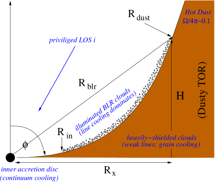
Figure 1: An illustration of the Bowl-shaped geometry. The BLR clouds occupy a region where gas is strongly illuminated by the central continuum source and line cooling dominates over either continuum cooling and grain cooling, effectively bridging the region between the outer accretion disc and the hot dust. The quoted hot dust covering fraction ($\Omega/4\pi\sim 0.1$) is taken from Landt et al. 2011b.

2 A Bowl-shaped BLR Geometry

In order to investigate the properties (gas distribution, kinematics, 1-d and 2-d response, profile shape etc) of bowl-shaped geometries as a class, we begin by first constructing a very simple toy model. For the purposes of illustrating the concept, we initially set the inner radius at 1 lt-day and outer radius at 10 lt-days and assume that the clouds lying near the surface of the bowl radiate isotropically, and do not cover one another (ie., have a direct view of the central continuum source). We parameterise the shape of the bowl in terms of the BLR scale height $H$ (in units of lt-days), such that

$$H=\beta R_{\rm x}^{\alpha}\,,$$ (1)

where $\beta$ and $\alpha$ are constants, $R_{\rm x}$ is the projected radial distance (in lt-days) along the plane perpendicular to the observers line of sight, ie. $R_{x}=R(\sin\phi)$, where $\phi$ is the polar angle (see figure 1). In the limiting case of zero scale-height, the normalisation constant $\beta$ is zero by definition, and the material lies along the mid-plane of the disc. For fixed (non-zero) $\beta$, the shape of the bowl is determined by the power-law index $\alpha$. The bowl is convex for $\alpha<1$, concave for $\alpha>1$, and cone-shaped for $\alpha=1$ (figure 2a). Note that $\phi$ is a function of radial distance $R$ unless $\alpha=1.0$, for which $\phi={\rm constant}$. When viewed along the axis of symmetry (down into the bowl), the spread in time-delays is minimised for fixed $\beta$, when $\alpha=2$, i.e. parabolic. For $\alpha>2$, gas lying near the surface of the bowl at larger radii will respond before gas at small radii (figure 2b). Since the time-delay, $\tau$, at radial distance $R$ is $\tau=R-H$, this condition will be met provided $\delta H>\delta R$ (or equivalently $d\tau/dR$ is negative). Note that in our model, we only observe the inner surface of the bowl, the outer surface being largely obscured from sight (since such sight lines would have to pass through the dusty TOR, see e.g. figure 1).

Figure 2: Bowl-shaped geometries with inner radius $R_{in}=1$ lt-day, outer radius $R_{out}=10$ lt-days, inclination $i=0$, and scale height $H$ (lt-days) and indicating (i) the shape (upper panels), and (ii) the range in expected delays (lower panels), for fixed $\beta$ (figures 2a, 2b), and fixed $\alpha$ (figures 2c, 2d).

The toy models discussed above, and illustrated in figure 2 serve as a tool for exploring how specific combinations of $\alpha$, $\beta$ determine the bowl shape, and the expected spread in time-delay for a fixed $R_{out}$. Since the formulism described leads to an infinite number of bowl shaped geometries, we restrict the parameter space further, by fixing both the BLR inner and outer radius ($R_{in}$, $R_{out}$), and the expected delay at the outer radius, $\tau(R=R_{out})$ (for $i=0$). Then, for a given choice of $\alpha$, $\beta$ is adjusted to match the specified delay at the outer boundary. In so doing, we can examine the properties of families of bowl-shaped geometries, with fixed radial extent, and with shapes differentiated by their chosen value of $\alpha$.

2.1 The BLR velocity field

For the velocity field, we assume that the gas motion is dominated by the gravitational potential well in which it sits, and is largely circularised, as might be expected in the presence of significant dissipative forces, such that:

$$v_{kep}^{2}=K\frac{R_{\rm x}^{2}}{(R_{\rm x}^{2}+\beta^{2}R_{\rm x}^{2\alpha})^{3/2}}\,,$$ (2)

where $v_{kep}$ is the local Keplerian velocity, $K=GM_{\rm BH}$, and $M_{\rm BH}$ is the mass of the central black hole. For the limiting case of a geometrically thin disc (ie. $\beta=0$), $v_{kep}^{2}=K\frac{1}{R}$, and the velocity field reduces to that expected for simple planar Keplerian orbits. Note that in this formulism, there is no radial component to the velocity field. Significant radial motion, either in the form of turbulence, or bulk radial motion may be introduced by the addition of an azimuthal perturbation to the velocity field (see §3.3).

While we do not exclude the possibility of infall, outflow (either centrifugal or radiation pressure dominated), or line-driven wind contributions to the BLR kinematics within individual AGN, we consider here the simplest possible and likely underlying scenario, of a largely gravitationally-dominated circularised flow. In particular we do not here consider the effects of a substantial wind contribution to the broad emission-line profiles of especially the high ionisation resonance lines, such as C iv (see e.g., the disc-wind models of Chiang & Murray 2006; Murray & Chiang 2007), which may be especially important in these lines in high Eddington rate AGN. We also note that while outflows, as manifested in blue-shifted UV and X-ray absorption lines (e.g., Elvis 2000) are common in AGN, their origin(s) is presently uncertain, although the inner TOR remains a plausible candidate (Pier & Voit 1995; Mullaney et al. 2008). Indeed the velocities reported for these outflows in Seyfert AGN (up to $\sim$1000 km s^-1, e.g., Crenshaw et al. 1999) roughly correspond with the expected gravitationally dominated velocities at the purported distance of the TOR. Moreover, in the sample of AGN with reverberation mapping data (e.g., Kaspi et al. 2000; Richards et al. 2011), there is no evidence for strong blue asymmetries in their C iv emission-line profiles, normally taken to be a strong indicator for outflows within the BLR.

Rather, we introduce macro-turbulent cloud motion (§3.3) as a simple, and often suggested, mechanism for providing a substantial radially-dependent scale height for the BLR clouds, allowing the BLR gas to intercept a significant fraction of the ionising continuum radiation necessary to produce the observed line strengths, something which remains problematic for thin-disc models of the BLR. In justifying our assumption, we note that the TOR which is the likely reservoir of gas that ultimately feeds the accretion disc, itself has a very large scale-height, while dynamical models of the BLR based on reverberation data appear to favour flared-disc geometries with substantial opening angles above the disc mid-plane (e.g. Pancoast et al. 2012, see §3.3 for details). Importantly in §3.2 we do investigate the effects of both transverse Doppler shift and gravitational redshift on the observed emission line profile and velocity delay map. A particular choice of $M_{BH}$, $R_{in}$, $R_{out}$, $\alpha$, and $\tau(R_{out})$ completely describes the BLR geometry and velocity field.

We emphasise that we do not advocate a fixed inner and outer boundary for the BLR nor do we mean to imply that the BLR forms the smooth inner surface of a bowl-shaped geometry. These are merely the simplest parameterisations of something which is very likely far more complex. Rather we aim to explore the observational consequences of assuming a bowl shaped BLR geometry in which the gas dynamics are dominated by the central super-massive black hole, and how these then impact on our interpretation of line profile shapes, correlated continuum and emission-line variability, velocity resolved response functions, black hole mass estimates and virial scale factors reported in the literature for both individual sources and among the AGN population as a whole.

3 A fiducial BLR geometry

To illustrate the general properties of bowl-shaped BLR geometries we construct a fiducial bowl-shaped geometry for the BLR for comparison with observations. For expedience we choose a parameter set appropriate for the Seyfert 1 galaxy NGC 5548. Our fiducial BLR geometry has a central black hole mass $M_{BH}=1.0\times 10^{8}~{}M_{\odot}$. We set the inner radius at 200 gravitational radii ($\approx$1.14 light-days for our assumed black hole mass) noting that the response time scales for He ii $\lambda$1640Å and N V $\lambda$1240Å are $\sim$2 days in NGC 5548 (Korista et al. 1995). We choose an outer BLR radius marking the upper rim of our bowl geometry of 100 light-days, roughly speaking the graphite grain sublimation radius (Nenkova et al. 2008) for our chosen continuum normalisation (see §4.1), and a maximum time-delay at the outer radius (for $i=0$) of $\tau=(R-H)/c=50$ days, similar to the dust reverberation time-delay measured for this object. With these parameters, the source covering fraction as determined from the polar angle to the bowl rim (60 degrees) is 50% for our fiducial BLR geometry.

We populate the bowl surface with discrete line emitting entities (hereafter, clouds) of fixed column density so that each cloud has an un-obscured view of the continuum source and radiates energy in a manner approximating the phases of the moon (see e.g., O’Brien et al. 1995, Goad 1995, Ph.D. thesis); we elaborate in §3.1. For simplicity, we ignore the effects of cloud–cloud shadowing in assuming an effective bowl surface, but do account for self-obscuration of the bowl by the outer rim (ie. lines of sight which pass through the obscuring dusty torus) which for this geometry occurs at inclinations $i>45$ degrees for $\alpha\ga 2$ (the bowl geometry power law index). We thus propose the bulk of the broad emission lines to form in gas clouds lying along an effective surface which spans between the accretion disc at small scale height and the TOR spanning a range in scale heights (see also Czerny & Hryniewicz 2011). The dimly illuminated gas clouds beyond the broad emission line region bowl surface are then likely dusty. The velocity field is described by equation 4 (discussed further in §3.3), and importantly we include the effects of Transverse Doppler Shift (hereafter TDS), Gravitational Redshift (hereafter GR), and turbulence on the emergent line profile (see §3.2 and §3.3).

Initially, we parameterise the radial surface line emissivity distribution $F(r)$ as a simple power-law in radius ($F(r)\propto r^{\gamma}$), with power-law index $\gamma=-1$ which is a fair approximation to the expected radial emissivity distribution derived from photoionisation calculations for several of the commonly observed UV and optical emission-lines (e.g., figure 9). We further assume that the line-emitting gas responds linearly to variations in the incident ionising photon flux $\Phi_{\rm H}$ (i.e., locally, the marginal response of the line to continuum variations remains constant with time). The spatially dependent line responsivity $\eta(r)$, is here defined as in Korista & Goad (2004), i.e.,

$$\eta(r)=\frac{\Delta\log F(r)_{line}}{\Delta\log\Phi_{\rm H}}$$ (3)

where $F(r)_{line}$ is the radial surface line emissivity, and $\Phi_{\rm H}$ is the incident hydrogen ionising continuum flux. For small amplitude continuum variations, this definition of responsivity converges to that given in Goad et al. 1993. Since we observe a spread in delays for lines of different species (see e.g., Clavel et al. 1991), in any given system, we focus here on bowl-shaped geometries parameterised by a bowl-shape power-law index $\alpha$ in the range $1\leq\alpha\leq 2.5$, noting that in geometries with $\alpha<1$, gas at larger radii will not have a direct view of the central continuum source, while gas at small radii on the near side is obscured from sight even at relatively small viewing angles, a consequence of the steepening of the bowl sides as $R$ decreases (increasing $dH/dR_{x}$).

In figures 3–6, we show the spatial distribution of BLR gas (as viewed from the azimuthal direction, R_z), the emissivity-weighted 2-d and 1-d response functions and steady-state line-profiles for bowl-shape power-law index $\alpha$ in the range $1.0\leq\alpha\leq 2.5$ (with the bowl geometry normalisation constant $\beta$ chosen to match the requirement that the maximum time-delay at the outer radius when viewed face-on is 50 days), and the fiducial geometry emission line profile as a function of the line of sight observer inclination, $i=$5, 10, 30, and 45 degrees. At large line-of-sight inclinations, the surface of the bowl becomes increasingly self-obscured since such sight lines must first pass through the surrounding dusty torus (the inclination at which self-obscuration first occurs decreases with increasing $\alpha$).

As expected the form of the 2-d response functions are broadly similar to those obtained for geometrically thin discs (the superposition of elliptical response functions) with a few notable differences. Firstly, as $\alpha$ increases, the fraction of surface area that lies at larger radii increases, so that the BLR response becomes increasingly weighted toward larger time-delays and thus lower line of sight velocities (e.g., figure 4 left–right). Furthermore, since rings at larger radii, are elevated with respect to those closer in, there is a smaller offset in time-delay between the centre of each ellipse than would be expected for a geometrically thin disc. This elevation of material out of the plane of the disc at larger radii, results in bowl-shaped geometries displaying enhanced response at small time-delays when compared to thin disc geometries with similar $R_{in}$, $R_{out}$. We note that for fixed $R_{out}$, the surface area of the bowl decreases with increasing scale height $H$, and increases with increasing $\alpha$.

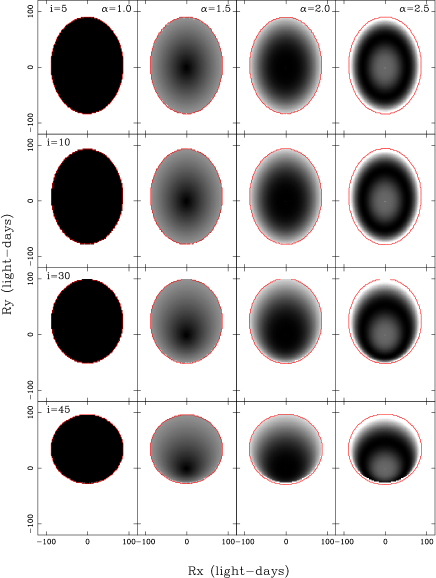
Figure 3: The spatial distribution of BLR clouds as viewed from the polar axis ($R_{z}$ direction). Individual panels show the expected cloud distribution for bowl-shape power-law index $\alpha$ in the range $1.0\leq\alpha\leq 2.5$, and inclination i=5,10,30 and 45 degrees. $\alpha=1$ represents a special case wherein individual clouds populate the surface of a cone. For our model, no shadowing is assumed to take place. The grey-scale represents the observed intensity (here normalised to the peak), for our adopted power-law emissivity distribution $F(r)\propto r^{\gamma}$, with power-law index $\gamma=-1$.

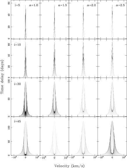
Figure 4: The corresponding 2-d response functions for figure 3.

The increased weighting toward larger radii with increasing $\alpha$ is most evident in the 1-d response functions. For $\alpha=1$, the 1-d response function is essentially flat with increasing time-delay, falling after a time-delay $R_{out}(1-\cos(\phi-i))$, corresponding to the light-crossing time of that part of the BLR which lies closest to the line of sight. At large $\alpha$, the increased weighting of the emissivity to larger radii (an area effect) causes the 1-d response function to peak at $R_{out}(1-\cos(\phi-i))$, moving towards smaller delays as $i$ increases. In the lower right panel of figures 4 and 5 the occultation of gas close to the line of sight results in the appearance of a secondary peak in the response function at small time-delays.

In all cases, the emission-line profiles are double-peaked, and broadly similar to those found for thin disc geometries. The locations of the peaks are as for thin disc geometries determined by the velocity at the outer radius (as given by equation 2), and the inclination $i$ (ie. $\pm v\sin i$). Obscuration by the surrounding dusty torus at large line of sight inclinations can be identified in the bottom right hand panels of figure 6, by the far larger difference in height between the line peaks and line centre and the U-shaped appearance of the line core, resulting from obscuration of low-velocity gas at large BLR radii and lying close to the line of sight.

While the parameter space to be explored is clearly large, figures 4–6 indicate that the emissivity-weighted 2-d and 1-d response functions and steady-state emission-line profiles are broadly similar for fixed observer inclination. Thus for the remainder of this work, we explore the observational characteristics of a single reference model, which we refer to as our fiducial BLR geometry, parameterised by bowl-shape power-law index $\alpha=2$ (corresponding to a normalisation constant $\beta=1/150$, for R and H measured in lt-days).

3.1 The role of emission line anisotropy and bowl scale height

For isotropically emitting gas orbiting in a geometrically thin disc, the centroid of the 2-d response function and the emission-line profile ’shape’ as quantified by the ratio $fwhm/\sigma_{l}$ in the absence of transverse Doppler shift (TDS) and gravitational redshift (GR) are independent of inclination. Furthermore, for our adopted line radiation pattern for individual clouds (which roughly speaking approximates a radiation pattern similar to the phases of the moon, e.g. O’Brien et al. 1994), increased anisotropy increases the centroid of the 2-d response function as $i$ increases, but the profile shape remains unaltered (reduced emission on the side nearest to the observer due to increased anisotropy in the line is replaced by enhanced emission on the far-side at the same velocity – front back symmetry).

By contrast for bowl-shaped geometries, the centroid of the 1-d response function increases with increasing observer line of sight inclination even for fully isotropically-emitting clouds (since rings on the bowl are pivoted about an axis running through the centre of the ring and the centre of the bowl). In addition, increased emission line anisotropy (see also Ferland et al. 1992) reduces the centroid of the 1-d response function at small inclinations (by reducing the contribution of gas at high elevations relative to that at low elevations), while increasing the centroid at larger inclinations due to the reduced contribution of gas closer to the observers line of sight. However, as for a thin disc geometry, front-back symmetry of our adopted line radiation pattern, yields line profile shapes which are independent of inclination in the absence of GR, TDS effects. Notably, for bowl-shaped BLR geometries, the centroid of the response function is a stronger function of inclination when compared with that for a standard thin disc geometry.

In practice we are mainly interested in geometries for which the line of sight inclination $i$ allows an un-obscured view of the bowl surface ($0\leq i<\phi$), that is, over the edge of the TOR. The BLR will be obscured on the near-side (closest to the line of sight) at larger inclinations either by self-occultation by BLR gas lying at larger radial distances, or by the surrounding TOR unless the line of sight to the central continuum source covering fractions of these components are themselves low. Indeed, low line of sight inclinations are suggested by a number of studies. X-ray studies of Seyfert 1 galaxies suggest BLR inclinations of $i\la 30$ degrees (Nandra et al. 1997, Nandra et al. 1999, Tanaka et al. 1995). Disc model fits to the double-peaked emission-line objects favour inclination angles of between 18–36 degrees (Eracleous et al. 1994). Furthermore, if the measured opening angles of ionisation cones observed in type 2 AGN are representative of AGN in general, then type 1 objects must be viewed at angles of $i<35$–60 degrees (Wilson and Tsvetanov 1994).

Figure 5: The corresponding 1d response functions for figure 3.

Figure 6: The corresponding line profiles for figure 3.

3.2 Transverse Doppler shift and Gravitational Redshift

At the inner radius chosen for our fiducial BLR geometry (200 $R_{g}$), the effects of transverse Doppler shift (hereafter, TDS) and gravitational redshift (hereafter, GR) have a significant effect on the emergent line profile, at low line of sight inclinations for the majority of lines, and in particular for those lines which form preferentially at small BLR radii. Using the standard formulism for each of these effects, we compare in figure 7 the 2-d response functions and emission-line profiles for our fiducial BLR geometry for inclinations i=5 and i=10 degrees, with (right panels) and without (left panels) the combined effects of TDS and GR (the 1-d response function is not shown here as it remains unaltered by the inclusion of these effects).

TDS and GR act to enhance the red wing response at small time delays (at the expense of the blue-wing response), thereby creating a strong red-ward asymmetry in the line profile. This effect is largest for small line of sight inclinations, since for our model, in the absence of turbulence, the line of sight velocity is zero at $i=0$, if the effects of TDS and GR are not included. GR effects will be most important for lines which form at small BLR radii (deep within the gravitational potential). Similarly for our chosen velocity field effects due to TDS will be stronger in lines which form at small BLR radii (e.g. compare figure 8 panels 5 and 6), where the velocities are more extreme. As shown in figure 7 the strong red-blue asymmetry introduced into the line profile is significant, as is the enhanced red wing response and diminished blue-wing response in the 2-d response function at small time-delays. At an inclination of 10 degrees, the importance of these effects diminishes (figure 7 – right panels, cf. dashed line), and at 30 degrees are barely detectable ($fwhm/\sigma_{l}\approx constant$ for $i>20$ degrees). A key result of this work, is that the effects of GR and TDS acting alone can provide substantial width to the emission-line ($\sim$ several hundred km s^-1), even for flattened, thin- or thick disc geometries, with pure planar Keplerian motion, viewed at low line-of-sight inclination.

In the absence of these effects line profile shapes as quantified by $fwhm/\sigma_{l}$ are independent of inclination in thin disc geometries. However, as we show in §6.1, in the context of flattened BLR geometries, when present GR and TDS introduce a strong inclination dependence to the line profile shape at low line of sight inclinations which matches both qualitatively and quantitatively the observed correlation between $fwhm/\sigma_{l}$ and $\sigma_{l}$ among AGN reported in the literature (e.g. figure 3 of Collin et al. 2006).

While Mannucci, Salvati and Stanga (1992) considered relativistic effects when modelling the 1-d response and emission-line profiles of disc- and nest-shaped BLR geometries, the effects of TDS and GR on the form of the 2-d response function have largely been overlooked. However, a prominent red-wing response is a key observational feature of the recently recovered 2-d response function for the optical emission-lines in the Seyfert 1 galaxy Arp 151 (Bentz et al. 2010b, their figure 4), though the response on the shortest timescales remain temporally unresolved. While these authors used the recovered response function to rule out a number of simple models for the BLR in this object, the effects of TDS and GR were not considered. If instead the enhanced red-wing response is a direct consequence of the combined effects of TDS and GR, then potentially Arp 151 may be a system with a low line-of sight inclination, or a system with significant emission at small BLR radii, for which the effects of TDS and GR are both larger.

Figure 7: Upper panels – 2-d response functions for our fiducial BLR geometry, with (right-hand panels) and without (left-hand panels) the combined effects of Transverse Doppler Shift and Gravitational Redshift. Lower panels – the corresponding 1-d line profiles. The dashed line in the right-hand side of panel 4 shows the same model without these effects (appearing in the left-hand side of panel 4).

3.3 Macro-turbulent cloud motion

For material to accrete, significant angular momentum must be removed via viscous dissipation outward through the disc. However, this process does not require the disc to be geometrically thin. Indeed, the relative ionising continuum and broad emission-lines fluxes require covering fractions for the BLR gas of at least 10%, and often substantially larger. This means that even for thin disc BLR geometries, the disc must have significant scale height in order to intercept sufficient ionising continuum necessary to explain the observed line strengths. Furthermore, moderately flared discs are predicted by standard accretion disc models (Shakura & Sunyaev 1973), and turbulence remains the simplest mechanism for supplying the internal pressure necessary to support the discs’ vertical extent. While the predicted scale heights for thin-disc geometries are rather modest ($H/R\sim 0.1$), in our model the BLR is not physically attached to the disc, though indeed it may be the originator of the BLR clouds. Instead we model the BLR as an ensemble of line-emitting clouds, and invoke macroscopic turbulent cloud motion as the mechanism which provides the BLR geometry with the necessary scale-height to intercept a substantial fraction of the ionising continuum. Recent dynamical models of the continuum and broad emission-line variations in the Seyfert 1 galaxy Mrk 50 (Pancoast et al. 2011), suggest flared discs with significant scale height ($\sim 0.5$ at the outer radius, for their assumed opening angle of $25\pm 10$ degrees) as a plausible geometry for this system. We also note that the surrounding TOR, which is the likely reservoir of material feeding the black-hole, itself must have substantial scale-height in order to obscure the BLR in type 2 objects (in the general orientation-dependent unified picture for AGN).

While GR and TDS provide substantial line width in thin disc geometries even for face-on objects, the line width is still largely determined by the black hole mass and source inclination. Thus for NLSy1s, which are thought to be low mass high accretion rate systems observed at low inclinations, a significant turbulent component may still be required to ensure sufficient width in the line.

In order to implement isotropic turbulence within the context of our model we add in quadrature a randomised velocity component $v_{\rm turb}$ which increases the local Keplerian velocity $v_{\rm kep}$ (equation 2) according to

$$v^{2}=v_{\rm kep}^{2}\left[1+\left(\frac{v_{\rm turb}}{v_{\rm kep}}\right)^{2}\right]\,,$$ (4)

and such that $|v_{\rm turb}|$ increases linearly with scale height $H$, i.e., $|v_{\rm turb}|=b_{\rm turb}\left(\frac{H}{R_{x}}\right)v_{\rm kep}$, where $b_{\rm turb}$ is a constant of order unity. This is similar to the implementation of turbulence with BLR scale height suggested in Collin et al. (2006). In practice, we draw at random a randomised (in direction) velocity vector from a Gaussian distribution of the appropriate width. Using this formulism, the turbulence is zero both when $b_{\rm turb}=0$ (turbulence switched off) and when $H=0$ (zero scale height). Thus in the context of bowl-shaped BLR geometries, the contribution that turbulence makes to the 2-d response function and line profile depends upon the bowl-shape, and on the radial surface line emissivity distribution which together determine the scale height at which a given line forms. Thus, in our model, the effects of turbulence are minimised for lines formed near the base of the bowl (small scale height). For non-zero $H$ and sufficiently large $b_{\rm turb}$, the randomised turbulent velocity component dominates over the planar Keplerian motion.

In figure 8 we illustrate the effects of turbulence on the 2-d response function and emission-line profile for our fiducial BLR geometry assuming a power-law emissivity distribution with power-law index $\gamma=-1$, and including the effects of TDS and GR, for an inclination i=5 degrees and turbulence parameter $b_{\rm turb}=1$ (left-hand panels), and $b_{\rm turb}=2$ (middle 2 panels). Turbulence has a number of important attributes. First, the lines are broader (as expected), and at low inclinations the prominent shoulders/horns indicative of flattened BLR geometries have disappeared even for moderate turbulence. Secondly, gas at large radii now makes a significant contribution to the line wings, enhancing the line wings relative to the line core. The effect of turbulence on line shape depends upon the size of $b_{\rm turb}$ and on the line formation radius. For example, as expressed in terms of the typically measured parameters used to quantify line profile shapes, the ratio of the line full-width at half maximum (hereafter $fwhm$) to the line dispersion (hereafter $\sigma_{l}$, see e.g., Collin et al. 2006), then for $b_{\rm turb}=0$, $\gamma=-1$ (dotted red line, lower left panel), $fwhm/\sigma_{l}$=1.4, increasing to 1.5 for $b_{\rm turb}=1$ (solid black line). For larger $b_{\rm turb}$, $fwhm/\sigma_{l}$=1.1 (lower middle panel, solid black line). While in panel 3, where we have now increased the radial power-law emissivity to $\gamma=-2$, $fwhm/\sigma_{l}$ increases from 1.0 without turbulence (dotted red line) to 1.4 with $b_{\rm turb}=2$ (solid black line).

We note that the observed lack of response of the broad emission-line wings on short time-scales in some objects has traditionally been explained by the presence of a low responsivity component in the inner BLR (see e.g., Goad et al. 1993; Sparke 1993; Korista & Goad 2004). Here, a similar effect arises for a different reason, a significant fraction of the broad emission-line wings, as observed at low inclinations, are now due to gas lying at large BLR radii which responds on longer time scales. If turbulence dominates the contribution to the emission-line response, then the core and wings of the line will respond on similar timescales.

One potentially significant result of this work is that at low inclinations, and in the presence of turbulence our model line profile displays a striking resemblance to a Lorentzian function. By way of illustration, we model the line profile with a 3-parameter Lorentzian of the form

$$I(x)=I_{0}\left[\frac{\Gamma^{2}}{(x-x_{0})^{2}+\Gamma^{2}}\right]\,,$$ (5)

where $I_{0}$ is the peak intensity, $x_{0}$ is the median velocity, and $\Gamma$ represents the half-width at half maximum of the line. Our best fit model shown in the lower middle panel of figure 8 (dashed blue line) with fit parameters, $I_{x=0}=1.025$, $\Gamma=623.5$ km s^-1, and $x_{0}=+82.2$ km s^-1 provides a remarkably good fit to the line profile, failing only in the extreme line wings which would in any case be difficult to measure in emission-line spectra due to their low contrast. The appearance of narrow cores and extended broad wings as observed in some type 1 Seyferts (in particular NLSy1s or “Pop A” objects; see Collin et al. 2006) may indicate the presence of significant turbulence and low inclination ($<20$ degrees) in these objects. While many studies have modelled the Balmer and Mgii emission line profiles with Lorentzians (e.g, Zamfir et al. 2010, their “Pop A” type 1 AGN), to our knowledge no explanation of why such profiles should manifest themselves has ever been offered, heretofore.

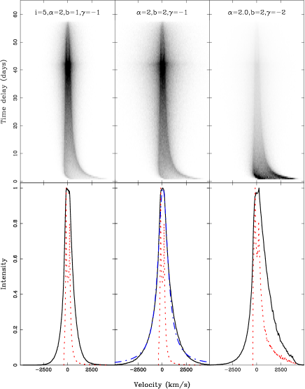
Figure 8: Upper panels - 2-d response functions for our fiducial BLR geometry with a line-of-sight inclination 5 degrees and turbulence parameter $b_{\rm turb}=1$, (left panel), $b_{\rm turb}=2$ (middle panel). In panel 3 we show $b_{\rm turb}=2$ for a power-law emissivity distribution with $\gamma=-2$. Lines formed at smaller scale height (with steeper emissivity distributions) are less affected by turbulence. Also shown (lower panels) are the steady-state line profiles (solid black lines), together with the expected profile for no turbulence, $b_{\rm turb}=0$ (red dotted line). In the middle lower panel we also show our best fit Lorentzian profile (blue dashed line) with fit parameters, $I=1.025$ , $\Gamma=623.5$ km s^-1, and $x_{0}=+82.2$ km s^-1.

For our model, turbulence is more significant for lines formed at larger BLR radii (e.g., H$\beta$, Mg ii), and hence larger scale heights. This is illustrated in figure 8 – right-hand panels, where we show the effect of steepening the power-law emissivity distribution to a slope of $-2$. The bulk of the line is now formed at small BLR radii, and thus small scale heights where the effect of turbulence is low. Consequently, though the turbulence parameter is large, a strong red-blue asymmetry, a result of TDS and GR whose effects are larger at small BLR radii, can still be discerned in the 2-d response function and emission-line profile. Thus at low line of sight inclinations, we expect to observe strong differences between the broad emission-line profiles of low- and high-ionisation lines.

In summary, TDS, GR and turbulence play a significant role in determining the shape of the 2-d response function and emission-line profile. Lines formed preferentially at small BLR radii will show an enhanced red-blue asymmetry in their 2-d response function and line profile due to the combined effects of TDS and GR (these effects will remain apparent provided the emission from the turbulent component does not dominate the contribution to the line profile). By contrast lines formed at large BLR radii will display more symmetric 2-d response functions and line profiles (because the effects of GR and TDS are diminished at larger BLR radii, and turbulence at larger scale height acts to reduce the dependence of line profile shape on inclination by randomising the velocity field). If turbulence is significant these lines’ emission-line profiles will show enhanced wings relative to the line core. For low inclination systems, turbulence produces Lorentzian profiles, especially in lines forming at large radii (e.g., Balmer and Mg ii) and so substantial scale height, similar to those seen in many NLSy1 (or “Pop A”) spectra. At higher inclinations, the Keplerian velocity dominates over the turbulent component, although the latter still affects especially the cores of the emission-line profiles (see Figures A1, A2). In light of these findings, we suggest that the previous association of an enhanced red-wing response with in-falling gas or a Keplerian disc + hotspot (for example, as suggested for the velocity field in the nearby NLSy1 Arp 151 (Bentz et al. 2010) and indeed spherical or disc-wind models of the BLR (Königl and Kartje 1994; Chiang and Murray 1996; Murray and Chiang 1997), may also in part be attributed to the presence of mildly relativistic gas in the inner BLR, as we have demonstrated here, as was previously suggested to account for the enhanced red-wing response observed in broad H$\beta$ for the Sy1 galaxy Mrk 110 (Kollatschny 2003b).

We note here that the recovered 2-d response function and emission-line profile for H$\beta$ in the NLSy1s NGC 4051 (Denney et al. 2011, their figure 4), Arp 151 (Bentz et al. 2010, their figures 2,3 and 4), and in the 2-d CCF of Mkn 110 (Kollatschny 2003, figure 7), bares an intriguing resemblance to that predicted for a bowl shaped geometry viewed close to face-on with a significant scale height dependent turbulent component (e.g., compare their figures with the left hand panel of Figures A1–A3 in Appendix A, for $i=10$ degrees). In Arp 151, an enhanced red-wing response is evident in all of the Balmer lines.

Significantly, GR, TDS and turbulence can on their own provide substantial line-width even for purely transverse motion and may explain the observed line widths in systems generally thought to be viewed close to face-on as well as the break in the $fwhm/\sigma_{l}$ relation at small $\sigma_{l}$ observed among the AGN population.

4 Simulations

4.1 Photoionisation calculations

Figure 9: (a) Radial emissivity distributions for selected low and high ionisation lines. The red line indicates a power-law emissivity distribution with power-law index $\gamma=-1$. (b) Radial surface responsivity distributions for selected low and high ionisation lines. The dashed vertical lines indicate the BLR inner and outer radius for our fiducial BLR geometry.

As in previous work, we adopt the most general model for the BLR gas, the locally optimally emitting cloud model of Baldwin et al. 1995 (see also Korista & Goad 2000, 2001, 2004). In brief, this model assumes that there exists a large population of BLR clouds with a broad range of gas density, gas column density, and ionising source distance. The observed broad emission-line spectrum arises by a process of natural selection, since for a given line only clouds whose properties span a relatively narrow range of physical conditions are efficient in re-processing the incident ionising continuum into particular line emission (hence “locally optimally emitting”, or LOC). This model not only explains why the observed spectra of AGN are generally similar, but significantly, requires minimal fine-tuning.

Using the photoionisation modelling code CLOUDY version c08.00 (Ferland et al. 1997, Ferland et al. 1998), we generated a grid of photoionisation models for simple slabs of gas (hereafter, clouds), each with a constant density and an un-obscured view of the ionising continuum source. In this simple approach contributions from the reprocessed continuum (the diffuse component from the cloud) and the effects of cloud shadowing are ignored. Moreover, we do not consider the complicating effects of micro-turbulence, which would tend to broaden the intrinsic line profile far above the thermal width and reduce the central line optical depth, thereby increasing the line escape probability isotropically (in this case) and hence altering the emergent spectrum (see e.g., Bottorff et al. 2000). This would also act to relax the requirement of large cloud numbers to explain the relative smoothness of the observed broad emission-line profiles (Arav et al. 1997; 1998). Of the four emission lines considered here (see Figure 9), micro-turbulence would affect mainly H$\beta$ and Mg ii, effectively moving their luminosity-weighted radii to smaller values.

The full grid spans 7 decades in the gas hydrogen number density–hydrogen ionising photon flux plane, $7<\log_{10}n_{\rm H}$ (cm^-3)$<14$, and $17<\log_{10}\Phi_{\rm H}$ (cm^-2 s^-1)$<24$, stepped in 0.25 decade intervals in each dimension (see also Korista et al. 1997). Since the emitted spectrum is not all that sensitive to the cloud column density over the range $22<\log_{10}N_{\rm H}$ (cm^-2)$<24$, all clouds are assumed to have a constant total hydrogen column density $\log_{10}N_{\rm H}$(cm^-2)$=23$. The adopted elemental gas abundances are solar. The adopted spectral energy distribution of the incident continuum is a modified form of the Mathews & Ferland (1987) generic AGN continuum. For the adopted mean ionising continuum source luminosity of NGC 5548, $\log_{10}L_{ion}=44.14$ erg s^-1, a hydrogen ionising photon flux $\log_{10}\Phi=20.0$ photon/s, corresponds to a cloud–ionising source distance of $R=15$ ($H_{0}$/70 km/s) light-days.

Utilising the standard LOC gas density distribution (weighting) function, $g(n_{\rm H})\propto n_{\rm H}^{-1}$, spanning the range in gas density $8<\log_{10}n_{\rm H}$ (cm^-3)$<12$, as described in Korista & Goad (2000; see also Baldwin et al. 1995; Bottorff et al. 2002), we sum the emission along the density axis for each radius, producing a radial surface line emissivity function (erg cm^-2 s^-1) for each of the lines considered. The radial surface line emissivity distributions are computed beyond the point at which grains will form, i.e., beyond the point where the grain temperature at the illuminated face of the cloud falls below the grain sublimation temperature. The radius at which this occurs ($\sim 100$ lt-days for our adopted continuum and the hardiest of grains) marks the inner boundary of the dusty TOR. For simplicity, we will assume the TOR to be opaque to UV/optical photons, and thus the central regions are obscured along lines of sight that pass through the TOR. The radial surface line emissivity distributions for C iv $\lambda$1549, Mg ii $\lambda$2798, H$\beta$ $\lambda$4861 and He ii $\lambda$4686 whose emission line profiles are commonly used in measuring black hole masses, are shown in figure 9(a) (solid black lines). For our fiducial model we assume a constant inward fraction for each of the lines (approximately a luminosity weighted-average) of 70% for C iv and He ii, and 80% for H$\beta$ and Mg ii, similar to the values determined for these lines over a broad range of physical conditions (e.g. O’Brien et al. 1994; Goad 1995, Ph.D. thesis; Korista et al. 1997a). For individual BLR clouds, we adopt a line radiation pattern which approximates the phases of the moon (see e.g., O’Brien et al. 1994).

In figure 9(b) we show the corresponding radial surface responsivities $\eta(r)$ (Eq. 3) for each line. These are derived from the radial surface line emissivities $F(r)$, by measuring locally the slope of this distribution and dividing by $-2$. Since the radial surface line emissivities are a function of the ionising photon flux and our choice of weighting in the $\Phi_{\rm H}$, $n_{\rm H}$ plane, so too are the radial surface line responsivities. However, some general trends do exist. For example, the responsivities of H$\beta$ and Mg ii are anti-correlated with the incident ionising photon flux, being stronger at low incident fluxes (in the outer BLR, where the optical depths are lower). This behaviour is also expected for He ii within the inner BLR (see figure 9). The C iv responsivity tends to align along lines of constant ionisation parameter (anti-correlating with $U=\Phi_{\rm H}/n_{\rm H}c$), but also gently declines for larger incident fluxes at constant $U$ for gas densities $n_{\rm H}\geq 10^{10}$ cm^-3 (see also Korista & Goad 2004, their figure 4).

4.2 The driving continuum light-curve

A model that describes the BLR gas distribution, must be able to reproduce the measured broad emission-line intensities and importantly their relative response to variations in the ionising continuum. While a single spectrum provides a “snapshot” of the physical conditions within the BLR, it is not a “true” representation of the current state of the line-emitting gas. This arises because the BLR is physically extended and therefore a single spectrum comprises contributions from gas in response to prior continuum states (due to the finite light-travel time across the BLR) up to and including the continuum state at the current epoch. Consequently, in order to compare the general characteristics of our fiducial bowl-shaped BLR model (see Table 1) with observations, we must first drive it with a model continuum light-curve whose variability power is representative of that determined for the source in question, taking into account both sampling effects and the finite duration of the light-curve (data sampling can be so sparse that the highest frequencies present in the underlying PSD are only poorly sampled by the observations). Our aim here is not to match the detailed response of individual lines, nor to fit the emission-line spectrum at a single epoch (for the reasons outlined above), rather here we aim to explore the gross properties of bowl-shaped geometries by determining the time-averaged spectrum and the average emission-line response timescale for the strongest UV and optical recombination lines for comparison with observations.

Here we adopt the approach of Kelly et al. (2009), and model the driving continuum light-curve as a damped random walk (see Kelly et al. 2009, and Macleod et al. 2010, for details), which has been shown to be an extremely good match to the variability of quasars (Kozlowski et al. 2010). We set the characteristic continuum variability timescale $\tau_{\rm char}$ to that measured by Collier and Peterson 2001, $\tau_{\rm char}=40$ days for NGC 5548, with a total duration of 450 days and daily sampling. The duration of our light curve is chosen to approximately match that of a typical monitoring season noting that the first $\tau_{max}$ points must be discarded since at prior times, the outer BLR has yet to respond to the continuum variations.

For each input continuum light-curve we compute the corresponding velocity resolved emission-line light-curve $L(v,t)$, assuming that locally, the emission-line gas responds linearly to continuum variations, i.e. a locally-linear response approximation (see Goad et al. 1993), so that while $\eta(r)$ remains time-independent, we now take into account the radial variation in line responsivity $\eta(r)$. As shown in Figure 9(b), and by Goad et al. 1993, the emission-line line responsivity shows a strong radial dependence. However, a locally linear response has been shown to be a reasonable approximation provided that the amplitude of the continuum variations are small (Goad, 1995, Ph.D. thesis, O’Brien et al. 1995). For larger continuum variations the locally linear response approximation is no longer valid and a full treatment of the time-dependent non-linear effects is required.

For each combination of continuum–emission-line light-curve we compute the peak and the centroid of their cross-correlation function (CCF, see e.g., Gaskell & Peterson 1987), for the latter adopting a threshold of 0.6 for the centroid calculation, as well as four different measures of the velocity field, the $fwhm$ and dispersion of the mean and root-mean square (hereafter rms) profiles, quantities that are commonly used by observers in the estimation of black hole masses using the reverberation mapping technique and/or scaling relations derived therein. To ensure that the full range in light-curve behaviour is sampled we repeat this process 1000 times and thereafter compute probability distribution functions for each of the measured quantities. In the following section we present the results of our simulations and place them within the context of results reported in the literature.

5 Results

Before exploring the effects of reverberation within the physically extended BLR on measurements of the continuum–emission-line delay and emission-line velocity dispersion, parameters typically used in virial mass estimates of the central black hole, we start by investigating an idealised case in which the predicted delay and velocity dispersion have been measured from the instantaneous 1-d responsivity-weighted response function and variable line profile. Such a situation would arise, for example, if the BLR were illuminated by a delta-function pulse rise in the ionising continuum flux. In so doing, we aim to reveal the relationship between the physical properties of our model (ie. our assumed geometry, emissivity, responsivity, velocity field, turbulence, and inclination) and the measured quantities used in black hole mass determinations.

The black hole mass estimates are here based on a virial product formed from the mean square dispersion, $\sigma_{l}^{2}$, of the variable line profile and the centroid, $\tau_{\rm cent}$, of the 1-d responsivity-weighted response function, such that.

$$M_{BH}=\frac{R_{blr}\delta v^{2}}{G}\,.$$ (6)

where $R_{blr}=c\tau_{\rm cent}$, and $\delta v^{2}=\sigma_{l}^{2}$. Since the black hole mass is an input to our model, it is straightforward to determine the virial scale factor $f$ required to force agreement between the measured black hole mass and the input value.

We have calculated virial masses, virial scale factors $f$, and line shapes for two pairs of emission-lines, H$\beta$–Mg ii, and C iv–He ii, chosen because they are representative of lines typically measured in ground- and space-based AGN monitoring campaigns, and importantly because they span a broad range in their characteristic line formation radii, and thus will probe the largest range in variability behaviour for our fiducial BLR geometry. We use the calculated radial surface line emissivity distributions of §4.1 (see figure 9), and adopt a locally-linear response approximation. We include the effects of anisotropic line emission, as described near the end of §4.1

5.1 The importance of turbulence, line emissivity, and inclination on $M_{\rm BH}$ determinations

To assess the impact of turbulence on the derived black hole masses and virial scale factor $f$, we have estimated $M_{\rm BH}$ for our fiducial BLR geometry for each of the four lines, for line-of-sight inclinations spanning the range 2–50 degrees and using 3 values for the turbulence parameter, $b_{\rm turb}=0$ (no turbulence), $b_{\rm turb}=1$ (moderate turbulence) and $b_{\rm turb}=2$. In figure 10 we show the virial mass estimates using equation 6 for each of the four emission lines (upper 4 panels), as well as the virial scale factor $f$ (middle 4 panels), required to reproduce the input black hole mass, as a function of line-of-sight inclination $i$. Individual colours indicate the degree of turbulence, $b_{\rm turb}=0$ (black line), $b_{\rm turb}=1$ (red line) and $b_{\rm turb}=2$ (green line). We find that in all cases, the estimated black hole mass is lower than the input mass, and is a strong function of inclination, being larger at larger line-of-sight inclinations. The middle 4 panels of figure 10 indicate that for a given inclination, and in the absence of reverberation effects, each line requires a different virial scale factor to recover the input mass. The discrepancy between the emission-lines is largest for zero turbulence and low line-of-sight inclinations. Additionally, black hole mass estimates are systematically lower and thus $f$-factors systematically higher with turbulence switched off (solid black line). The discrepancy between the virial mass estimate and the input mass can be larger than 2 dex for near face-on systems with turbulence switched off. For lines which form at large BLR radii, corresponding to a larger scale height in our model, e.g. H$\beta$, Mg ii, turbulence significantly enhances the black hole mass estimates at low line of sight inclinations (solid green line), reducing the discrepancy between the virial mass estimate and the input mass by more than 1 dex. This arises because for our chosen velocity field, in the absence of turbulence, the line width at small line-of-sight inclinations is a result of the combined effects of TDS and GR only. Turbulence in our model acts to increase the local velocity field at large scale heights thus broadening the emission-line and thereby increasing the virial mass estimate and consequently lowering the virial scale factor. Since in our model turbulence increases with increasing scale height this effect is more pronounced in lines which form at large BLR radii (e.g. H$\beta$, Mg ii). Furthermore, turbulence randomises the direction of the velocity field and thereby acts to reduce the otherwise strong dependence of the emission-line width on inclination, normally found for planar Keplerian motion.

In the lower panel of figure 10 we show the emission-line shape ($fwhm/\sigma_{l}$) as a function of line $fwhm$ (or equivalently line-of-sight inclination $i$). This reveals a strong dependence of emission-line shape on line $fwhm$, such that broader lines have more Gaussian profiles, while narrower lines are more Lorentzian in shape. In general turbulence acts to soften the otherwise strong dependence of line shape on inclination. However at low line-of-sight inclinations, turbulence dominates over the planar Keplerian motion moving low velocity gas from the line core to the line wings, resulting in profiles with narrower cores and extended line wings ($fwhm/\sigma_{l}<1$). Once again, this effect is most pronounced in lines which form at large BLR radii (e.g. H$\beta$, Mg ii). Figure 10 indicates that for lines formed at small scale heights (C iv and He ii), the effect of turbulence on the derived $M_{\rm BH}$ and $f$-factors is significantly smaller.

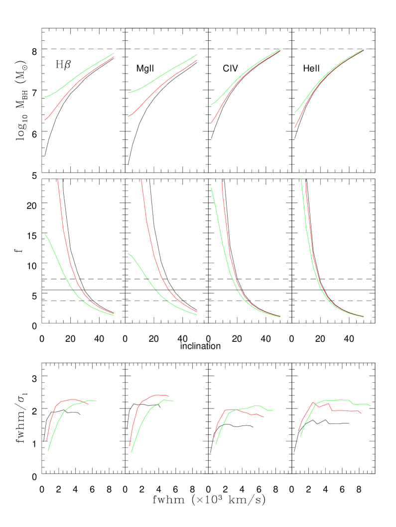
Figure 10: Panels 1–4 – $M_{\rm BH}$ as a function of line of sight inclination $i$ for each line for our fiducial BLR geometry and 3 values of the turbulence parameter, $b_{\rm turb}=0$ (black line), $b_{\rm turb}=1$ (red line) and $b_{\rm turb}=2$ (green line). Mass estimates are here based on measurements of the mean-square dispersion of the steady-state (mean) line profile and centroid of the 1-d responsivity-weighted response function. Panels 5–8 – the corresponding virial scale factors, $f$ also as a function of inclination $i$. Panels 8–12 – dependence of line shape $fwhm/\sigma_{l}$ as a function of line $fwhm$ (for the same 3 values of $b_{\rm turb}$).

Onken et al. (2004) showed that nearby AGN for which both reverberation based and velocity dispersion based mass estimates are available, follow the same $M_{BH}-\sigma$ relation as quiescent galaxies. From this they derived a statistical estimate of the virial scale factor for all AGN with reverberation mapping data, finding an average $f$-factor of $f=5.49\pm 1.65$ for H$\beta$, see also Table 2 of Collin et al. (2006), here indicated by the horizontal solid and dashed lines (middle panel of figure 10). Woo et al. (2010) provide an updated value for the virial scale factor $f$. Their estimate $\log f=0.72\pm 0.1$ is based on matching reverberation masses of 24 AGN with those obtained from recent stellar velocity dispersion estimates of the host galaxy, adopting the $M_{\rm BH}-\sigma$ relation of quiescent galaxies from Gültelkin et al. (2009), and is consistent within the errors with that found by Onken et al. (2004). We note that for our fiducial BLR geometry, the inclusion of a scale height dependent turbulent component, increases the range in inclination returning viral scale factors that are consistent within the errors with the average $f$-factor for H$\beta$ reported by Collin et al (2006) and Woo et al. (2009).

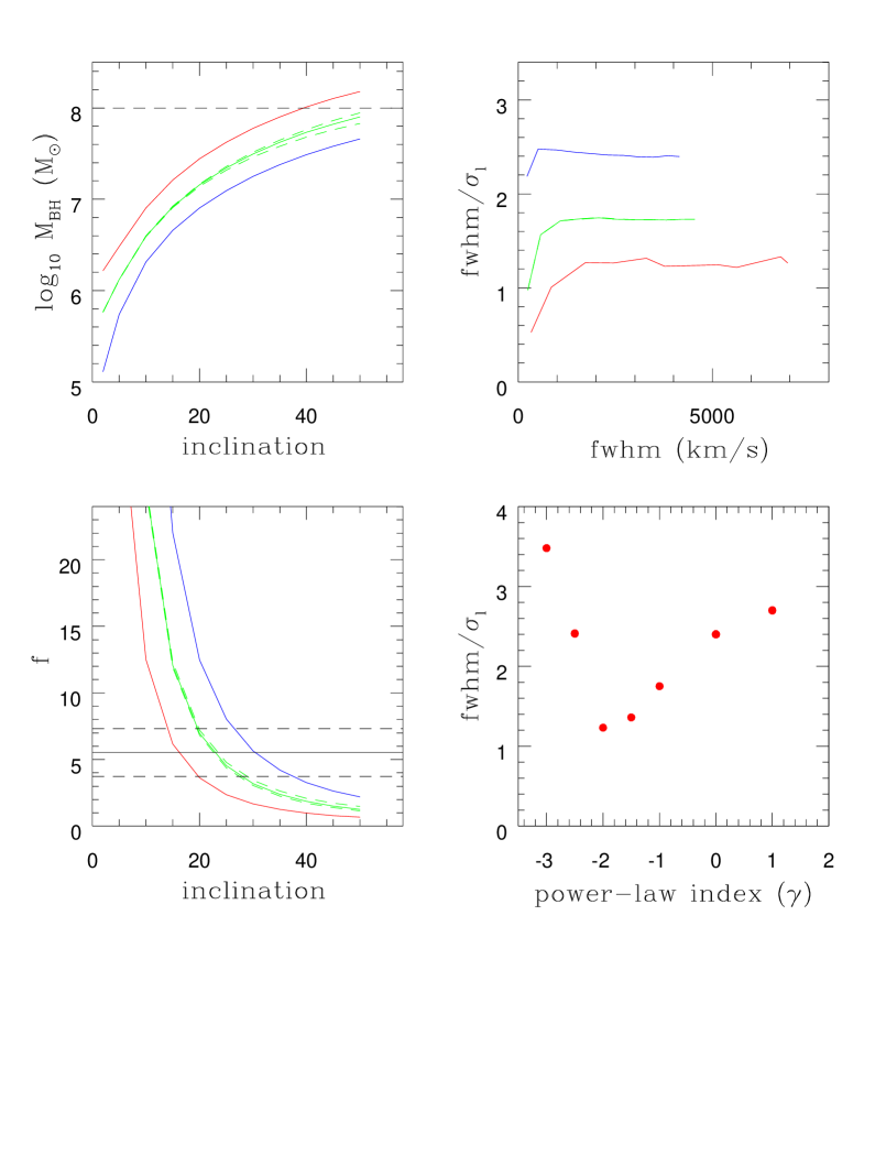
Figure 11: Panel 1 (upper left) – $M_{\rm BH}$ as function of inclination for a geometrically thin disc and power-law emissivity distribution with power-law index $\gamma=0$ (blue lines/symbols), $-1$ (green) and $-2$ (red). Also shown (green dashed lines) is the effect of changing the line radiation pattern (for $\gamma=-1$) from 50% (isotropic)–100% (anisotropic). Panel 2 (lower left) - corresponding virial scale factors. Panel 3 (upper right) - corresponding line profile shapes as a function of $fwhm$. Panel 4 (lower right) $fwhm/\sigma_{l}$ as a function of power-law emissivity index $\gamma$. Differences in the ratio $fwhm/\sigma_{l}$ between lines may result from differences in their radial surface emissivity distributions. N.B. a geometrically thin disc has a very small scale height by construction, and thus the turbulent velocity is effectively zero even though we chose $b_{\rm turb}=2$.

For completeness we show in the left hand panels of figure 11 the derived black hole mass and virial scale factor, $f$, as a function of inclination for a geometrically thin disc with the same inner and outer radius as our fiducial BLR geometry (1.14 and 100 light-days respectively), turbulence parameter $b_{\rm turb}=2$, and using simplified power-law line emissivity distributions with power-law index $\gamma=0$ (solid blue line), $-1$ (solid green line), and $-2$ (solid red line). We also show (dashed green lines) the effect of changing the line anisotropy from 50% (ie. isotropic, $F_{inwd}=\frac{1}{2}F_{totl}$) to 100% (ie. anisotropic, $F_{inwd}=F_{totl}$). Line anisotropy increases the emissivity-weighted radius by a factor $1+\frac{1}{2}\sin^{2}i$, (Goad 1995, Ph.D. thesis, O’Brien et al. 1994), and thus for the limited range of inclinations studied here results in a marginal increase in the virial scale factor for a geometrically thin disc. As for our bowl-shaped geometry the masses are systematically underestimated (except at large inclination and for steep emissivity distributions – red line, upper left-panel) and the discrepancy between the calculated and input black hole mass decreases with increasing inclination. The thin disc model also shows a significant change in profile shape at small inclinations (figure 11, upper right panel). Since a disc by construction has little scale height, the contribution of the turbulent component is minimal (even though $b_{\rm turb}=2$). Thus for a given radial surface line emissivity distribution, only GR and TDS can play a significant role in modifying the line shape for thin-disc geometries at small inclinations. We note that in the absence of these effects, the emission-line shape is independent of inclination for our adopted emission-line radiation pattern. Of more significance is the strong dependence of the mass estimates on the radial surface line emissivity distribution, which indicates that in the absence of turbulence, lines which are preferentially formed at small BLR radii yield larger black hole masses, and thus smaller virial scale factors. A similar result was found for our fiducial model (figure 10 – solid black lines, cf. H$\beta$–Mg ii and C iv–He ii). We discuss this further in the following section.

Finally, we note that unless turbulence dominates the velocity field, then for a bowl-shaped BLR geometry, we expect to observe a strong $f$–$fwhm$ dependence in all lines regardless of where they form (due to the strong dependence of $fwhm$ on inclination), and broadly similar to that found for disc-like configurations (see Decarli et al. 2008, their figure 6). Scatter in the relation between different lines may point to differences in their radial surface line emissivity distributions and/or the presence of a significant turbulent velocity component.

5.2 $fwhm/\sigma_{l}$ - the role of emissivity

As noted by Collin et al. (2006) the ratio of the zeroth and 2nd order moments (mean and root mean square respectively) of the broad emission-line profile can be used to place constraints upon the BLR geometry and kinematics. Decarli et al. (2008) found that in a sample of 36 AGN with roughly equal numbers of radio-loud and radio-quiet objects, that the ratio $fwhm/\sigma_{l}$ for H$\beta$ is closer to that derived for an isotropic BLR geometry (wherein $fwhm/\sigma_{l}=2.35$), while the smaller values ($\approx 1$) measured for C iv are more suggestive of a flattened BLR geometry. Combined with the strong correlation between their virial scale factor $f_{d}$ and $fwhm$ found for both lines (such a correlation is expected if line of sight velocity is a strong function of inclination), and the absence of a correlation between the $fwhm$ of H$\beta$ and C iv, Decarli et al. (2008) argue that their results are consistent with C iv originating in a flattened BLR geometry, with H$\beta$ originating in a geometrically thick disc with a significant turbulent component. As in our model, the increased turbulence at large scale height reduces the dependence of the H$\beta$ line width on inclination and therefore could account for the reported absence of a correlation between the H$\beta$ and C iv emission-line widths, the more isotropic appearance of the H$\beta$ line profile, and if the turbulence is large enough, the larger width of H$\beta$ relative to C iv.

However, we caution here that the ratio $fwhm/\sigma_{l}$ for fixed $R_{in}$, $R_{out}$ has a strong dependence on the radial surface line emissivity distribution. For example, if we approximate the radial surface line emissivity distribution as a power-law in radius ($F(r)\propto r^{\gamma}$), then for a geometrically thin disc, the ratio $fwhm/\sigma_{l}$ is a minimum for $\gamma=-2$, and increases for both smaller and larger $\gamma$ (see figure 11, lower right panel). For $\gamma$ large and positive, the emission is weighted toward the outer edge only, yielding $fwhm/\sigma_{l}\approx 2.8$ as appropriate for a ring-like distribution. Similarly, for negative $\gamma$, the inner radius dominates the emission, while emission from rings at larger radii (and hence lower velocity), tend to fill in the dip at line core (between the horns) producing more rectangular-looking profiles (smaller $fwhm/\sigma_{l}$). In extreme cases ($\gamma<-3$), this can lead to $fwhm/\sigma_{l}>3$. For our fiducial model, C iv has a steeper emissivity distribution than H$\beta$ and thus a smaller $fwhm/\sigma_{l}$ (cf. figure 10 – lower panels 1 and 3, and figure 11 – upper right panel), which may in part explain the differences found by Decarli et al.(2008). A similarly strong dependence of line shape on radial surface line emissivity distribution can be found for other BLR geometries (see also Robinson 1995a,b) Thus while differences in the ratio of $fwhm/\sigma_{l}$ between H$\beta$–C iv may indicate differences in their scale height, we suggest that differences in their radial surface line emissivity distributions likely also play a significant role. Evidence in support of this claim comes from the large range (factor of a few) in $fwhm/\sigma_{l}$ displayed by the H$\beta$ line in NGC 5548 during 13 years of monitoring (Collin et al. 2006). Since in an individual source neither the black hole mass nor its inclination can change appreciably on such a short timescale, this suggests that the observed variations in the Balmer line profile shape for NGC 5548, over the 13 years of observation, are due to gross changes in the radial surface line emissivity distribution in response to large variations in the ionising photon flux within the physically extended BLR, though we cannot rule out dynamical changes on longer baselines ($\sim$several years for NGC 5548).

Figure 12: H$\beta$ (hashed lines) and He ii CCF centroid (left panels) and peak (right panels) distribution functions (resulting from 1000 simulated continuum–emission-line light-curves) for a range of BLR inclinations. Also shown is the centroid of the 1-d response function for H$\beta$ (vertical dashed line) and He ii (vertical dotted line) as determined from the steady-state model.

Table 1: Our fiducial BLR model.

$M_{BH}$	$R_{min}$	$R_{max}$	$\tau(R_{max})$	$\alpha$	$\beta$	$b_{\rm turb}$
($M_{\odot}$)	(lt-days)	(lt-days)	(lt-days)
$10^{8}$	1.14	100.0	50.0	2.0	1/150	2.0

5.3 The importance of Reverberation: Which measures of $R_{blr}-\delta v$ should be used?

In order to assess the impact of continuum–emission-line reverberation on the virial mass estimates and hence scale factors $f$, we have driven our fiducial BLR geometry, with simulated continuum light-curves whose variability characteristics have been designed to match those observed in the best studied AGN, the Seyfert 1 galaxy NGC 5548. Our fiducial BLR model (see Table 1 for details) utilises the computed radial surface line emissivity distributions for each line (§4.1), our prescription for emission-line anisotropy and line radiation pattern (§4.1), and a turbulence parameter $b_{\rm turb}=2$. All simulated emission-line light curves have been calculated assuming a locally-linear response approximation. For each of the four lines considered (H$\beta$, Mg ii, C iv and He ii), we compute their velocity resolved time-variable emission-line light-curve $L(v,t)$, and their mean and root mean square (rms) emission-line profiles.

Simulations were performed for a range of line of sight inclinations i=2,5,10,20,30,40, and 50 degrees, and repeated 1000 times, in order to ensure that the full range in continuum variability behaviour is sampled and to allow the construction of probability distribution functions in each of the desired quantities that we wish to measure. For each continuum – emission-line light-curve combination we have calculated the peak and centroid of the cross-correlation function (figures 12–13). Additionally, from the velocity resolved time-variable light-curve, we have constructed mean and root-mean square profiles from which measurements of their full width at half maximum ($fwhm$) and line dispersion ($\sigma_{l}$) have been determined. Thus, from each simulation we have two estimates of the continuum–emission-line delay (or characteristic size of the BLR), and four estimates of the velocity dispersion (two from the mean profile and two from the rms profile). From these we construct eight estimates of the BLR mass in the standard fashion using equation 6.

Figure 13: As for figure 12 for Mg ii (hashed area) and C iv.

For a few individual objects, intensive ground and space-based spectroscopic monitoring campaigns have been employed to determine black holes masses under the assumption of virialised gas motion for broad emission-lines spanning a broad range in ionisation state (e.g. Clavel et al. 1991, Ulrich et al. 1991, Peterson et al. 1991, Krolik et al. 1991). For NGC 5548 Peterson and Wandel (1999) showed that while lines of differing ionisation state display differences in both their line dispersion and response timescale they all appear to follow (more or less) the same virial relation. Furthermore, Peterson et al. 2004, and Collin et al. 2006, using 13 years of monitoring data of the optical emission-lines in NGC 5548 showed that differences in the measured lags and line widths from one season to the next yielded virial products which are effectively constant within the errors, demonstrating that the reverberation masses while not necessarily accurate, are at least robust (reproducible). However, as noted by these authors, it is not immediately obvious which of the measured quantities (CCF peak or centroid, $fwhm$, $\sigma_{l}$ of the mean or rms profile) yield the most accurate black hole masses, nor which of the emission-lines should be used in mass determinations.

Theoretical considerations suggest that measurements from rms profiles rather than mean profiles should yield more accurate estimates of the virial product, since they isolate the variable part of the emission-line from non-variable components (Fromerth and Melia 2000). However, because of the lower S/N of rms profiles, a consequence of the small variability amplitude, measurements from rms profiles tend to be more uncertain. Collin et al. (2006) argued that provided the non-varying components can be isolated from the mean profile, then the mean profile should yield estimates of the virial product of a similar precision. Additionally, Peterson et al. (2004) showed that the line dispersion $\sigma_{l}$ can be measured with greater precision than the line $fwhm$ and provides a better match to the virial relation, which suggests that estimates of the virial product based on $\sigma_{l}$ should have smaller uncertainty. Finally, the centroid of the CCF, equivalent to the centroid of the 1-d response function (or the emissivity-weighted radius for a linear response) is the generally preferred quantity used for estimating the ’size’ of the BLR since it is less sensitive to the inner BLR radius than is the peak of the CCF (Peterson et al. 1998), but see Welsh 1999, for an alternative viewpoint. Indeed, for objects in which monitoring campaigns have been performed for multiple lines, Peterson et al. 2004 found that the tightest virial relation was found for virial products determined from measurements of the centroid of the CCF ($\tau_{cent}$) and the line dispersion ($\sigma_{l}$) of the rms spectrum.

In summary, from an observational perspective virial products based on measurement of the CCF centroid and the dispersion of the rms profile remain the quantities of choice. However, it seems at least plausible that the choice of these quantities may simply reflect limitations in the observational data, be it signal–noise or sampling. Here we attempt to address the question as to which of the measured quantities and for which lines yield the most accurate black hole masses from a modelling perspective.

5.3.1 CCF centroid or peak

In terms of the measured delay, or characteristic size of the BLR, it has long been known that the CCF peak (or lag) is a less reliable measure of the characteristic BLR size than is the centroid, and tends to be biased towards the inner BLR radius (see e.g. Edelson and Krolik 1988; Pérez, Robinson and de la Fuente 1992; Melnikov and Shevchenko 2008) though see Welsh 1999 for an alternative point of view. By contrast, the centroid of the CCF is directly related to the centroid of the response function (the responsivity weighted radius, Koratkar and Gaskell 1991) and thus should be a more accurate representation of the ’size’ of the region responding to continuum variations (the correspondence is not exact even for the centroid and depends strongly on the continuum variability behaviour exhibited during the observing campaign, see e.g. Pérez, Robinson and de la Fuente 1992).

Figures 12–13 show the distribution in the measured delay in terms of both the centroid and peak delay (or lag) for each line over a range of BLR inclinations. Also shown is the centroid of the 1-d responsivity-weighted response function (vertical dotted line for He ii and C iv, vertical dashed line for H$\beta$ and Mg ii) for the steady-state for the same inclination. For low inclinations the CCF centroid for all lines bar He ii tracks the centroid of the response function reasonably well, while for larger inclinations ($i>10$ degrees), the measured centroid displays larger scatter and is systematically smaller than the true centroid in all lines. The discrepancy between the centroid of the 1-d responsivity-weighted response function and the centroid of the CCF is notably worse at large inclinations for He ii and C iv, which in our model preferentially form at small BLR radii. Furthermore while at low inclinations the peak of the CCF also tracks the centroid of the response function reasonably well, it performs far worse at larger inclinations. For He ii the peak delay is systematically smaller than the centroid of the 1-d response function regardless of inclination. Our adopted continuum variability timescale of 40 days is close to the centroid of the 1-d response function for H$\beta$ and Mg ii respectively and is the most likely explanation for their improved performance in tracking the continuum variations when compared to C iv and He ii, particularly at large inclinations.

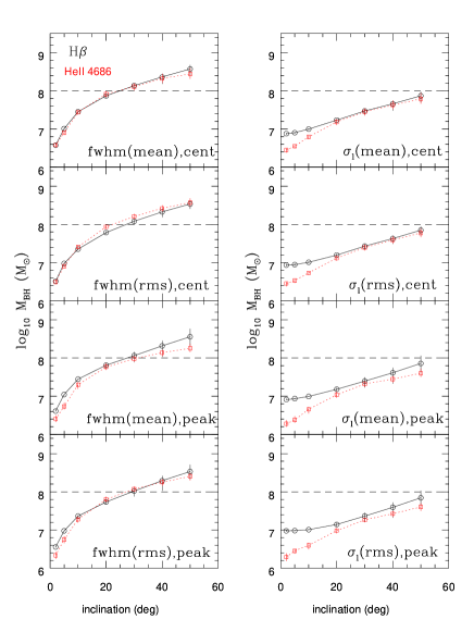
Figure 14: 8 estimates of the black hole mass, $M_{BH}$ (median, and 1$\sigma$ confidence interval) based on the virial product $R_{blr}\delta v^{2}/G$ as a function of inclination $i$ for our fiducial BLR model (see Table 1), and based on 1000 simulated light-curves at each inclination. Our calculated virial products (Eqtn. 6) employ two measures of $\delta v$, $fwhm$ and $\sigma_{l}$, and two measures of $R_{blr}$ ($\equiv c\tau$), the CCF centroid and CCF peak. Together these provide 4 estimates of $M_{BH}$ for both the mean and rms profiles (giving 8 estimates in total). Individual panels show results for H$\beta$ (open circles, solid black line), and He ii $\lambda$4686 (open squares, red dashed line).

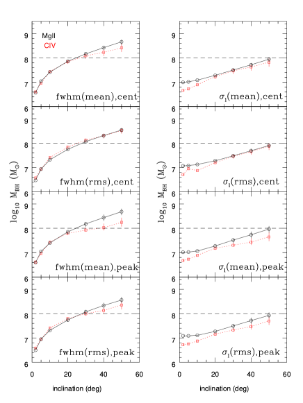
Figure 15: As for figure 14, but now showing the results for Mg ii $\lambda$2798 (open circles, solid black line), and C iv $\lambda$1550 (open squares, red dashed line).

5.3.2 Mean or rms profiles

Figures 14–15 show the derived black hole mass distribution functions (8 independent estimates) as a function of line of sight inclination $i$ for all four lines. Because the mass distribution functions are typically skew the points and their errors here represent the median and 68% confidence limits respectively. The input black hole mass is indicated by the horizontal dashed line. As expected, the derived $M_{\rm BH}$ for all four lines shows a strong dependence on inclination, with black hole mass estimates systematically lower than the input mass at low line of sight inclinations. Mass estimates based on measurements using the line $fwhm$ (from both the mean and rms profile) show a greater dependence on inclination at small inclinations, than do mass estimates based on measurements of the line dispersion $\sigma_{l}$ (ie. as noted by Collin et al. 2006, $\sigma_{l}$ is a less biased indicator of mass).

For our model, $fwhm/\sigma_{l}\approx 1$ at i=2 degrees, and increases to a maximum for inclinations $i>20$ degrees after which time $fwhm/\sigma_{l}$ is approximately constant (see also figure 10). Thus the line shape is largely insensitive to inclination effects at large inclinations but is a strong function of inclination at small inclinations ($i<$ 20 degrees), inclinations for which scale-height dependent turbulence may significantly modify the line profile (see § 5.1). The origin of this effect in our model is due entirely to the implementation of Gravitational redshift and transverse Doppler shift (see §5.1). In the absence of these effects, only the line width (and not line shape) is a strong function of inclination.

Since $fwhm/\sigma_{l}>1$ for all lines (except at the lowest inclinations) mass estimates based on measurements of the $fwhm$ are generally larger than those based on $\sigma_{l}$. Black hole mass estimates based on the line $fwhm$ systematically underestimate the mass at low line of sight inclinations, while systematically overestimating the mass for line of sight inclination $i>20$ degrees (see figures 14–15). Mass estimates based on measurements of the line dispersion, $\sigma_{l}$, systematically under-predict the black hole mass at all inclinations and for all lines, with the largest discrepancies at the lowest inclinations. The larger scatter in measurements of the $fwhm$ and $\sigma_{l}$ of the rms profile is as expected (a reverberation effect), but does not necessarily lead to a larger scatter in the derived mass, if variations in the line widths are compensated for by corresponding changes in the measured delay.

The use of CCF centroid or peak in the virial relation in general makes only a small difference to the estimated masses (see e.g. left-hand or right-hand panels of figures 12–13) though the exact behaviour depends both on the line in question and details of the continuum variability behaviour during a single model run. For example, for He ii the CCF centroid is on average larger than the CCF peak at all inclinations, while for C iv, the CCF centroid is on average larger than the CCF peak only for $i>10$ degrees. Similarly, for H$\beta$, the CCF centroid is on average larger than the CCF peak for inclinations in the range $10<i<50$ degrees, and smaller than the CCF peak otherwise. For Mg ii the CCF centroid is on average larger than the CCF peak for inclinations in the range $5<i<30$ degrees, and smaller than the CCF peak otherwise. Thus when considering all lines, we expect to find on average larger black hole masses at large inclinations when using the CCF centroid, while at low inclinations the CCF centroid yields lower mass estimates than the CCF peak for all lines except He ii.

We have recast the derived $M_{\rm BH}$ from our reverberation simulations of our fiducial BLR model to illustrate the variation in virial scale factor $f$ as a function of inclination for each line. Here we restrict ourselves to four estimates only, the four used by Collin et al. 2006, in which velocity dispersion measurements ($fwhm$, $\sigma_{l}$) have been taken from the mean and rms profiles, and the centroid of the CCF is used as a proxy for BLR size. The results of this exercise are displayed in figure 16, where the points and their errors once again indicate the median and 68% confidence limits respectively. Increasing the characteristic variability timescale for the continuum variations from 40 to 80 days only marginally alters the virial scale factor for H$\beta$ (smaller for the line dispersion and larger for the line $fwhm$).

Figure 16: Four estimates of the virial scaling factor f, for four different lines driven by 1000 continuum light-curves with a characteristic variability time scale $\tau_{\rm char}$ of 40 days. Black filled circles (H$\beta$), blue triangles (Mg ii), green squares (C iv), and cyan crosses (He ii). The horizontal solid and dashed lines represent the average H$\beta$ scale factors, $f$(H$\beta$) and their uncertainties, as derived for the Onken et al. sample by Collin et al. 2006.

Continuum variability blurs the differences between the predicted virial scale factors for each line to the point at which they are virtually indistinguishable within the errors at inclinations larger than $\approx$20 degrees. Thus when measurement errors are included we predict little if any difference between the $f$-factors (or mass estimates) derived for different lines. Importantly, $f$-factors derived from the $fwhm$ of the rms and mean profile show significantly less scatter and a closer correspondence between the lines than those based on $\sigma_{l}$, particularly at low inclinations. This consistency between mass estimates for different emission lines derived using the line $fwhm$ has been confirmed observationally (Assef et al. 2011). Because our light curves are well-sampled, there is only a small spread in the measured values of $fwhm$ and $\sigma_{l}$ of the mean profile. Thus the dispersion in the computed virial scale factors from measurements of mean profiles is mostly due to variations in the location of the centroid of the CCF. For light-curves which are only sparsely sampled, we would expect larger variations in $fwhm$ and $\sigma_{l}$ in the mean profiles, though still smaller than those measured for rms profiles. Figure 16 shows that for mass estimates based on measurements of the line $fwhm$, the $f$-factors for all lines are consistent within the errors ($f\pm\delta f$) with those reported by Collin et al. (2006) for inclinations in the range $20<i<35$ degrees. For estimates based on measurements of the line dispersion $\sigma_{l}$, the acceptable range narrows to $20<i<30$.

The average virial scale factor for the Decarli et al. sample is $f_{d}=1.6\pm 1.1$ for H$\beta$ and $f_{d}=2.4\pm 0.16$ for C iv, that is $f$-factors tend to be larger for C iv than H$\beta$. For our fiducial model, in the presence of turbulence $f$(H$\beta$)($\sigma_{l}$) $<$ $f$(C iv)($\sigma_{l}$) for $i<20$ degrees for both the mean and rms profile (figure 16), because of the stronger dependence of the H$\beta$ line width on turbulence due to it forming at preferentially greater distances and scale height. By contrast $f$-factors derived from the $fwhm$ of the mean and rms profile indicate $f$(C iv)($fwhm$)$\approx$ $f$(H$\beta$)($fwhm$), though the correspondence is generally worse for the lowest inclinations.

The larger scatter in the $f$-factor between the low and high ionisation lines at low $i$ derived using $\sigma_{l}$ (figure 16 – left hand panels) highlights the reduction in sensitivity of the line-dispersion to inclination in the presence of strong turbulence (which mainly effects the low ionisation lines). We suggest that objects for which the lines show large differences in their virial scale factors (as derived using the line dispersion) may be indicative of low inclination sources.

6 Discussion

A bowl-shaped BLR geometry provides an elegant solution to the smaller than predicted dust reverberation sizes by decreasing the measured delays without altering the dust formation radius. At the same time, since material now lies away from the observers line of sight, they readily reproduce the observed lack of response on short timescales evident in the 1-d and 2-d response functions of the strong optical recombination lines.

Differences in the radial surface emissivity distribution and line anisotropy among the low and high ionisation lines in the context of a bowl-shaped BLR, results in large differences in the form of the 1-d response functions at fixed inclination (see figure A3, appendix). For geometrically thin discs, the characteristic variability timescale as determined from the centroid of their 1-d response functions is independent of inclination for isotropically emitting clouds, and increases with inclination otherwise. For bowl-shaped geometries, the centroid of the 1-d response function increases with inclination even for isotropic emission. Moreover for the radiation pattern adopted here, at small inclinations, increased line anisotropy can reduce the centroid of the response function relative to the isotropic case due to the reduced contribution of gas at large elevations which lies closer to the line-of-sight.

While the LILs show an absence of response on short timescales in their 1-d response function, the 1-d response functions for the HILs, which are formed at smaller BLR in a more flattened distribution, resemble those of disc-shaped BLR geometries, with a significant response even on short timescales (though the response does decline to zero at zero delay). Thus this model reproduces the observed differences in the location of the peak response among low and high ionisation lines reported in the literature (e.g., Krolik et al. 1991, their figure 10 and 11). We note that here we have assumed a locally linear line response and that the precise form of the 1-d response function may be modified in the event of significant non-linear effects (this may include a luminosity-dependent continuum shape as well as the incident continuum flux-dependent effects already mentioned).

The additional effects of GR and TDS enhance the red-wing response producing line profiles with extended red-wings, as are sometimes observed in type 1 AGN (Kollatschny 2003). The strength of the red-blue asymmetry depends primarily on the line formation radius, being stronger for lines formed at small BLR radii (i.e., steep radial emissivity distributions). GR and TDS together provide significant line width ($\sim$ several hundred km s^-1) even for face-on geometries with pure-planar Keplerian motion. More importantly, GR and TDS introduce a strong inclination dependence to the line profile shape at low inclinations. In the absence of these effects the shape of the emission-line profiles are independent of inclination for flattened/bowl-shaped BLR geometries assuming isotropic emission, though of course their line widths will show a strong inclination dependence (the observed line of sight velocity, $v_{obs}$, varies as $v\sin i$).

Mass determinations for flattened/bowl-shaped BLR geometries show a strong dependence on inclination particularly at small inclinations where the mass estimates are systematically smaller than the input model. In general, when reverberation effects are included, mass estimates based on measurements of the $fwhm$ underestimate the mass at low inclinations, and overestimate the mass at high inclinations, while those based on measurements of the line dispersion $\sigma_{l}$, systematically underestimate the mass at all inclinations. Mass estimates based on measurements of the emission line $fwhm$ (rms or mean profile) are larger since in general $fwhm/\sigma_{l}>1$. Our model also confirms the result of Collin et al. 2006, showing that mass estimates based on measurements of $\sigma_{l}$ are less biased than those determined from measurements of the $fwhm$, because of the weaker dependence of $\sigma_{l}$ on inclination, particularly at low inclinations. For our simulations, we find a better correspondence between mass determinations derived from different lines particularly at low inclinations, if measurements of the virial product are performed using the $fwhm$ of the mean or rms profile. The form of emission line anisotropy adopted in this model leaves the profile unchanged, but causes the characteristic response timescale for the line to increase with increasing inclination. This effect is smaller than the corresponding increase in velocity with inclination and consequently both $M_{\rm BH}$ and $f$ are only weakly dependent on line anisotropy (e.g. figure 11, lower left panel).

Turbulence, as implemented here, modifies the shape of the 2-d response function and emission-line profile, by moving lower velocity gas that responds on long timescales to larger line of sight velocities (hence broadening the lines). The overall effect on line shape is line dependent, and is largely determined by the line formation radius, so that while turbulence may increase the ratio $fwhm/\sigma_{l}$ for lines formed at small BLR radii (small scale heights), the general effect is to reduce $fwhm/\sigma_{l}$ for lines formed at large BLR radii (large scale heights), so that at low line of sight inclinations, the line profiles are characterised by narrow cores and extended line wings (i.e., Lorentzian), similar to those seen in NLSy1s, see figure 8 and §5.1 for a full discussion of these effects. Because turbulence randomises the velocity field, turbulence acts to reduce the $v\sin i$ dependence of the line dispersion in flattened BLR geometries.

To summarise, in the absence of turbulence, emission-lines with steeper emissivity distributions yield : (i) larger estimates for the central black hole masses, (ii) smaller virial scale factors (f-values) and (iii) smaller $fwhm/\sigma$ (see e.g. figure 10).

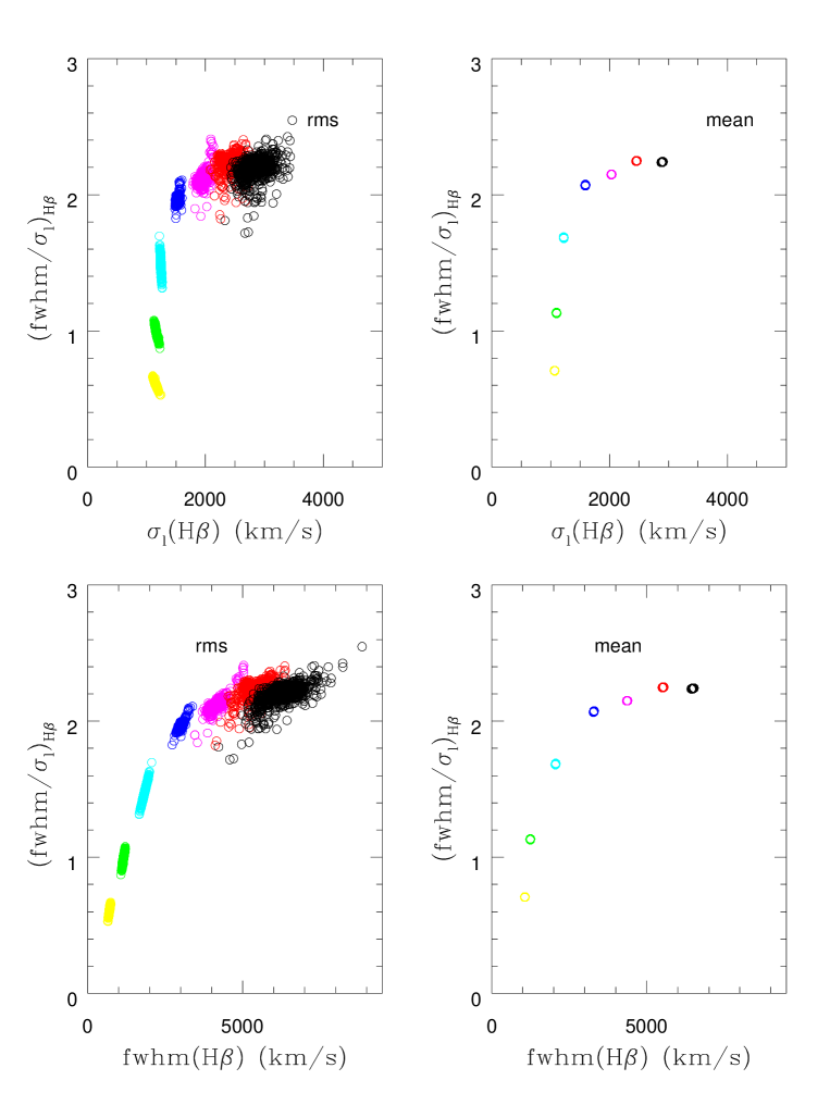
Figure 17: $fwhm/\sigma_{l}$(H$\beta$) versus (i) $\sigma_{l}$(H$\beta$) (top panels), and (ii) $fwhm$(H$\beta$) (lower panels) for the rms (left hand panels) and mean profiles (right hand panels) for our fiducial bowl-shaped model with turbulence parameter $b_{\rm turb}=2$, driven by 1000 simulated continuum light-curves, and observed at line of sight inclinations 2 (yellow open circles), 5 (green), 10 (cyan), 20 (blue), 30 (magenta), 40 (red), and 50 (black) degrees. At a given inclination the rms profile shows a larger range in $fwhm/\sigma_{l}$, a consequence of reverberation within the spatially extended BLR. A far smaller range is seen for $fwhm/\sigma_{l}$ at fixed inclination for the mean profile, as measured from the same simulations (same number of points). For $i>20$ degrees, the profile shape is largely independent of inclination.

6.1 Line shape as an orientation indicator

Collin et al. 2006, showed that the shape ($fwhm/\sigma_{l}$) of the broad H$\beta$ line in reverberation mapped AGN varies by a factor of a few, and tends to be smaller in Narrow Line objects ($fwhm/\sigma_{l}<2.35$) than in Broad Line objects ($fwhm/\sigma_{l}>2.35$), where $fwhm/\sigma_{l}=2.35$ is the value appropriate for a Gaussian profile. The boundary separating the narrow line and broad line objects, hereafter population 1 and population 2 sources, roughly corresponds to a $\sigma_{l}$ of 2000 km/s, and is broadly similar to the division of AGN into population A population B sources by Sulentic et al. (2000). In the latter scheme, population A sources have profiles characterised by narrow cores and broad wings (ie. are more Lorentzian in shape) while population B sources appear more flat-topped (i.e., more Gaussian).

By estimating the virial product using $fwhm$ and $\sigma_{l}$ of the mean and rms profiles of each sample and comparing to the $M_{BH}$ values obtained using stellar velocity dispersion measurements for the same AGN, Collin et al. (2006) calculated virial scale factors for both Pop 1/A and Pop 2/B samples, as well as the sample as a whole. A key result of their work is that the virial scale factor determined from measurements of the line dispersion (mean or rms profile) is independent of line shape, or AGN type. By contrast, virial scale factors based on the line $fwhm$ show significant differences among the different AGN populations (pop 1/A, pop 2/B) and is thus a more biased estimator of the velocity dispersion.

Collin et al. (2006) speculate that the factor of $\approx 3$ difference in the virial scale factor derived using the $fwhm$ for population 1/A and population 2/B sources may be due to the increased sensitivity of the $fwhm$ to inclination effects or Eddington ratio, since population 1/A sources tend to be high Eddington rate sources. They suggest that the rapid decrease in $fwhm/\sigma_{l}$ at small $\sigma_{l}$ arises in a 2-component BLR, comprising a disc component producing the emission-line core, and an isotropic (possibly a wind) component producing the line wings. Since the core of the emission-line is more sensitive to the $fwhm$ and arises in a flattened configuration, it will show a strong dependence on inclination. Conversely, the wings of the line are more sensitive to $\sigma_{l}$, and arise in an isotropic component which is inclination independent. We here offer an alternative explanation. The rapid decrease in $fwhm/\sigma_{l}$ at small $\sigma_{l}$ arises naturally in planar disc-like (thin or thick) geometries in which the effects of GR and TDS are taken into consideration. At small inclinations $\sigma_{l}$ is independent of inclination while the ratio $fwhm/\sigma_{l}$ increases rapidly (factor of $\sim$ 5). That is, the line $fwhm$ is more sensitive to changes in inclination for small inclination angles than is the line dispersion. This effect can be seen more easily in figure 17 where we show the ratio $fwhm/\sigma_{l}$ for H$\beta$, as measured from the mean and rms profiles (left and right-hand panels respectively) as a function of $\sigma_{l}$ (upper panels) and $fwhm$ (lower panels). At low inclinations $i<20$ degrees, $\sigma_{l}$ is effectively constant. Variations in line shape are then entirely due to changes in the line $fwhm$ (compare the upper and lower left panels of figure 17). At higher inclinations, the line shape is nearly independent of inclination. This trend is seen in measurements from both the mean and rms profiles. The reduced scatter in the ratio $fwhm/\sigma_{l}$ for the mean profile relative to the rms profile, suggests that measurements taken from the mean profile are less sensitive to reverberation effects with the spatially extended BLR. Turbulence shifts all velocities to higher values while its effect on $fwhm/\sigma_{l}$ depends on the scale height at which the line forms. For large turbulent values $fwhm/\sigma_{l}$ tends toward 2.35 (a Gaussian profile), as appropriate for a randomised velocity field. In any event, it is difficult to see how the bottom right hand corner of figure 17 can be populated in this model, in agreement with observations (see Collin et al. 2006, their figure 3; Kollatschny & Zetzl 2011, figures 1–3; Peterson 2011). Remarkably, for our model the break toward smaller $fwhm/\sigma_{l}$ occurs at a $\sigma_{l}$ of between 1500 and 2000 km/s, similar to the boundary between population 1 and population 2 sources defined by Collin et al. 2006 (see also Peterson 2011). Figure 17 shows the range in profile shape as a function of $fwhm$ and $\sigma_{l}$ for a single source with fixed $M_{\rm BH}$, viewed at a range of line of sight inclinations and in the presence of reverberation effects (ie. approximating the results of many observing seasons). By comparison, Figure 3 of Collin et al. (2006) indicates the mean profile shape observed in AGN which differ in both $M_{\rm BH}$ and line of sight inclination. Yet our figure 17 and figure 3 of Collin et al. are remarkably similar in appearance. Increased mass will tend to shift points in the upper left panel of Figure 17 toward higher velocity dispersion, effectively filling in the left hand side, while leaving the line profile shape at larger velocity dispersions, virtually unchanged, as is observed. Similarly, the lower left panel of Figure 17 bares a striking resemblance to Figure 1 of Kollatschny and Zetzl (2011). Yet in their model a Lorentzian component was input by hand, while here it arises naturally in low inclination systems for lines formed at large BLR radii and in the presence of scale height dependent turbulence.

As expected reverberation effects can alter the emission line profile shape, though for our simulations the range in $fwhm/\sigma_{l}$ at a fixed inclination is by comparison with NGC 5548, relatively modest ($\sim$10–20%). We suggest that the far larger range in $fwhm/\sigma_{l}$ observed over the 13 year monitoring campaign of NGC 5548, which at times crosses the boundary between population 1 and population 2 sources, is a consequence of changes in the radial surface line emissivity distribution in response to changes in the ionising continuum flux. We also find that at a fixed inclination the range in $fwhm$ as determined from the rms spectrum is far larger than that for $\sigma_{l}$ (figure 17 left panels), suggesting that in our model, the line dispersion is also less sensitive to reverberation effects within the physically extended BLR. The far smaller spread in $fwhm$ and $\sigma_{l}$ for the mean spectra (figure 17 – right panels) is mainly due to the absence of contaminating non-variable components and the fact that the light-curve is uniformly sampled with no gaps between observations.

6.2 Anomalous narrow-line quasars

In a recent study on anomalous narrow-line quasars from the Sloan digital sky survey, Steinhardt & Silverman 2011 (arXiv:1109.1554) showed that the virial masses determined using the familiar scaling relations derived for the broad H$\beta$ and Mg ii emission-lines differ by up to 0.5 dex in these objects. ANLs are identified by a broadened narrow H$\beta$ line relative to Mg ii. This broadened narrow-line component is found to be well-correlated with broad H$\beta$ in these objects. Since H$\beta$ and Mg ii are expected to form under similar physical conditions, one would normally expect a similar relation to be evident in Mg ii. Steinhardt & Silverman 2011 argue that the absence of such a correlation in Mg ii may cast doubt as to the validity of virial mass estimates based on measurements of the H$\beta$ line width, arguing that some of the broadening may be due to the presence of a wind. Thermal emission from a wind lacking an ionisation front would produce an additional H$\beta$ component without contributing significantly to the Mg ii emission.

Bowl-shaped geometries may provide an alternative solution. If as expected Mg ii forms at large radial distances, and turbulence is significant at large scale heights, then one can envisage a situation in which the Mg ii emission is dominated by a turbulent component. The Mg ii line width would then be largely independent of inclination effects. By contrast if H$\beta$ emission arises at smaller radial distances (smaller scale heights), the lower turbulence and more flattened spatial distribution would ensure a strong inclination dependence even at modest inclinations (GR and TDS are less important for these lines due to their larger formation radii). Thus, ANLs may represent near face-on objects with a significant turbulent component in the Mg ii forming region.

7 Summary

We have explored the observational characteristics of a class of broad emission line region geometries in which the line emitting gas spans the region between the outer accretion disc and the inner edge of the dusty torus, by occupying an effective (though not necessarily smooth or continuous) surface the scale height of which increases with increasing radial distance (ie. a bowl-shaped BLR geometry), similar to the configuration first proposed by Gaskell (2009). A Type 1 AGN spectrum is then observed for line-of-sight viewing angles which peer over the rim of the bowl. Such a configuration provides quite naturally the necessary high covering fractions for the observed emission-line strengths, without obscuring the view of the central engine (for a reasonable range in line-of-sight viewing angles). The gas dynamics are here assumed to be dominated by gravity, and we include in our model the effects of gravitational redshift, transverse Doppler shift and scale-height dependent turbulence. While we do not exclude possible contributions from infall, outflow, or line-driven wind contributions to the BLR kinematics within individual AGN, we consider here what is most likely the underlying and dominant effect of a gravitationally bound BLR velocity-field consisting of circularised orbital motion, as might be expected if there are significant dissipative forces acting within the BLR. Importantly, we introduce a macroscopic turbulent component to the cloud motion which imparts substantial scale height to the BLR at large radii, allowing it to intercept sufficient ionising continuum radiation to explain the observed emission-line strengths.

By breaking spherical symmetry, a bowl-shaped geometry simultaneously provides a simple solution to the shorter than predicted dust reverberation timescale for the inner dusty torus and the absence of a significant response of the broad optical recombination lines on short timescales. Gravitational redshift and transverse Doppler shift offer a mechanism for providing substantial line width, even in the case of purely transverse motion. They also introduce a strong red-blue asymmetry into the 2-d response function and emission-line profile in the form of an enhanced red-wing response at short time-delays similar to that seen in the recently recovered 2-d emission-line response function and emission-line profile of the NLSy1 Arp 151 (Bentz et al. 2010, Brewer et al. 2011). These effects are most important for lines with steeper radial emissivity distribution which therefore form at small BLR radii (the HILs, e.g. He ii, C iv) and for those systems viewed at low line of sight inclination. Differences in the line formation radius between the high- and low-ionisation lines lead to strong differences in the shapes of their 2-d and 1-d emission-line response functions and emission-line profiles.

While the LILs show a deficit of response on short-timescales, the HILs, which form toward the base of the bowl in a more flattened configuration, show significant response on short-timescales, and their 2-d and 1-d response functions appear similar to those found for geometrically thin discs. Additionally, GR and TDS for flattened BLR geometries (ie. bowl-shaped, thick or thin disc geometries), result in line profile shapes which display a strong inclination dependence at low line of sight inclinations, with $fwhm/\sigma_{l}$ decreasing with decreasing $i$. At larger inclinations, the line profile shape is nearly independent of inclination. Thus inclination, in the presence of GR and TDS may provide a natural explanation for the observed differences in line profile shapes among AGN in general and importantly may also explain the observed differences in the line profile shapes used to discriminate between pop A and pop B sources (Sulentic et al. 2000, Collin et al. 2006). We suggest that some of the systems previously identified as high Eddington rate sources based on their profile shape, may simply be type 1 objects viewed at low line of sight inclinations. We note that the break between inclination dependent and inclination independent line profile shapes ($\sigma_{l}\approx 2000$ km/s, see figure 17) is remarkably similar to the boundary separating the high- (pop A) and low- (pop B) Eddington rate sources. Also, we speculate that high Eddington rate sources may have TORs with larger than typical covering fractions, necessitating smaller observed viewing angles $i$ for un-obscured lines of sight.

For a bowl-shaped BLR with significant scale-height dependent turbulence, we expect the low-ionisation lines (e.g. H$\beta$, Mg ii) to display line shapes which are more Gaussian in shape (larger $fwhm/\sigma_{l}$) than the high ionisation lines (e.g. C iv, He ii), as is observed (Decarli et al. 2008). This arises because the low-ionisation lines form at larger BLR radii (and hence larger scale heights) where the turbulent (random) contribution to the velocity field is larger. By contrast the high-ionisation lines form at small BLR radii (near the base of the bowl) where the turbulent component is substantially reduced (for example, compare the $fwhm/\sigma_{l}$ as a function of inclination $i$ for the low- and high-ionisation lines with and without turbulence, figure 10 lower panels). As can be seen, as well as significantly broadening the line profile, turbulence softens the strong dependence of line profile shape on inclination at low inclinations for the low-ionisation lines. By moving low velocity gas (at large BLR radii) to larger line of sight velocities, turbulence removes the strong horns and shoulders characteristic of pure planar Keplerian motion while reducing any delays that may be present between the wings and core of the line. For low line of sight inclinations, the turbulent contribution to the line of sight velocity is larger than the Keplerian contribution (for motion confined to the disc mid-plane) and turbulent broadening acts to produce emission line profiles which are Lorentzian in form ($fwhm/\sigma_{l}\approx 1$, e.g. figure 8), with extended broad wings and narrow cores. As far as we aware, this is the first study to provide physical motivation for the fitting of emission-line profiles using Lorentzians. A significant scale-height dependent turbulent component may help explain the reported weakness in the correlation between the measured widths of the low- and high- ionisation lines (e.g., H$\beta$ and C iv). In cases of sufficiently large contributions from this component, H$\beta$ might even be broader than C iv, a finding which when taken at face value, appears at odds with what one would normally expect based on photoionisation calculations of a gravitationally bound BLR.

A strong motivation for this work was to try to identify which lines and which of the measured quantities yield the most accurate and most reproducible mass estimates for $M_{BH}$. The time-stationary model indicates that :

1. Different emission lines predict different virial mass estimates and hence different virial scale factors (figure 10).

2. Mass estimates made from measurement of the emission line $fwhm$ show a strong inclination dependence, leading to an underestimate of $M_{BH}$ at low inclinations, and an overestimate of $M_{BH}$ at large inclination. The largest discrepancies are for low line of sight inclinations and in the absence of turbulence for lines formed at large BLR radii (ie. the LILs, see figure 10).

3. Mass estimates made from measurement of the emission line dispersion $\sigma_{l}$, underestimate $M_{BH}$ at all inclinations, but show a much weaker dependence on $i$ than the $fwhm$ (see also figures 14–15), confirming the results of Collin et al. (2006), that mass estimates based on $\sigma_{l}$ are less biased.

4. Measurements of the emission line $fwhm$ (mean or rms profile) predict larger $M_{BH}$ than measurements based on $\sigma_{l}$, since in general $fwhm/\sigma_{l}>1$, except at the smallest inclinations.

5. In the presence of turbulence, black hole mass estimates based on measurements of emission lines formed at large BLR radii (ie. H$\beta$, Mg ii), are less sensitive to inclination effects than those formed at small BLR radii (ie. C iv, He ii), and for which the turbulent contribution to the velocity field is weaker.

6. In the absence of turbulence, emission lines formed at small BLR radii (ie. the HILs) yield larger $M_{BH}$ (figure 10) and therefore smaller virial scale factors.

When the effects of emission-line variability are taken into account, we find that:

1. The cross correlation function (CCF) centroid tracks the continuum variations more closely than the CCF peak, and shows a better correspondence with the centroid of the emission line response function in lines whose variability timescale is more closely matched to the characteristic variability timescale of the driving continuum (ie. the LILs, figures 12–13). However, the choice of CCF centroid over CCF peak has little overall effect on the predicted mass.

2. The best correspondence between $M_{BH}$ estimates (and hence $f$-factors) for different lines, arises from measurements of the $fwhm$ of the mean or rms profile, consistent with results reported in the literature from observations (e.g. Assef et al. 2011). The stability of the mean profile suggests that measurement of the $fwhm$ of the mean profile is the preferred estimate of $M_{BH}$ (figure 16).

3. The largest discrepancy between the derived virial scale factors between different emission lines arise from measurements of $\sigma_{l}$ in low inclination systems ($i<20$ degrees, figure 16). We suggest that some of the systems previously identified as high Eddington rate sources based on the shapes of their low-ionisation emission lines, may simply be more typical type 1 objects viewed at low line of sight inclinations.

Our findings at first glance appear at odds with those presented in Peterson et al. (2004) who found that the tightest relation between the virial products derived for different lines in a single source is found for those estimated using the CCF centroid, and the line dispersion of the rms spectrum. Note that the difference here is that we calculate the time-delay (centroid or peak) of the CCF and line width ($\sigma_{l}$ or $fwhm$) of the mean and rms profile for 1000 realisations of the driving continuum light-curve, and not the variation in centroid and line width within a single realisation. Due to the long duration of our light-curves, any biases introduced by windowing effects are minimised. In addition, the model presented here utilises a locally linear response approximation. Gross changes in the radial surface line emissivity distribution and in the inner and outer radius in response to large variations in the ionising continuum flux variations will be treated elsewhere (Goad and Korista, in prep.).

A comparison between the H$\beta$ virial scale factors presented in our simulations and the empirically estimated virial scale factors based on the AGN with reverberation data presented in Collin et al. (2006) suggests a rather narrow range of typical inclination angles for Type 1 objects, $i\approx$ 20–35 degrees or so, in agreement with the expected range found via other techniques.

8 Acknowledgements

We would like to thank the anonymous referee for providing comments which have led to improved clarity of the work presented here. Mike Goad and Kirk Korista would also like to thank the generous hospitality of Keith Horne and the Department of Physics & Astronomy at the University of St. Andrews during the initial stages of this work. Kirk Korista would like to thank the Department of Physics & Astronomy at the University of Leicester for their generous hospitality during his stay during the major stage of this work. Mike Goad would like to thank Dr Graham Wynn for many useful discussions.

9 References

Antonucci, R. 1993, ARA&A 31, 473.

Arav, N., Barlow, T.A., Laor, A. and Blandford, R.D. 1997, MNRAS, 288, 105.

Arav, N., Barlow, T.A., Laor, A., Sargent, W.L.W., and Blandford, R.D. 1998, MNRAS, 297. 90.

Assef , R.J., Denney, K.D., Kochanek, C.S., Peterson, B.M., Kozlowski, S. et al. 2011, ApJ 742, 93.

Baldwin, J. Ferland, G. Korista, K.T. and Verner, D. 1995, ApJ 455, L119.

Barvainis, R. 1987, ApJ 320, 537.

Bentz, M.C., Denney, K.D., Cackett, E.M. et al. 2007, ApJ 662, 205.

Bentz, M.C., Horne, K., Barth, A.J. et al. 2010, ApJ 720, l46.

Bentz, M.C., Walsh, J.L. Baarth, A.J. et al. 2010, ApJ 716, 993.

Bottorff, M. Korista, K.T. Shlosman, I. and Blandford, R.D. 1997, ApJ 479, 200.

Bottorff, M., Ferland, G., Baldwin, J. and Korista, K. 2000, ApJ 542, 644.

Bottorff, M.C., Baldwin, J.A., Ferland, G.J., Ferguson, J.W. and Korista, K.T. 2002, ApJ 581, 932.

Brewer, B.J., Treu, T., Pancoast, A., Bart, A.J., Bennert, V.N. et al. 2011, ApJL 733 L33.

Chiang, J. and Murray, N. 1996, ApJ 466, 704.

Clavel, J. Reichert, G.A., Alloin, D. et al. 1991, ApJ 366, 64.

Collier, S., and Peterson, B, M. 2001, ApJ 555, 775.

Collin, S., Kawaguchi, T., Peterson, B.M. and Vestergaard, M. 2006, A&A 456, 75.

Corbin, M.R. 1997, ApJ, 485, 517.

Crenshaw, D., Kraemer, S.B. Boggess, A. et al. 1999, ApJ 516, 750.

Czerny, B., & Hryniewicz, 2011, A&A, 525, L8.

Decarli, R., Labita, M., Treves, A., and Falomo, R. 2008, MNRAS 387, 1237.

Denney, K.D., Peterson, B.M. Pogge, R.W. Adair, A. et al. 2009, ApJ 704, L80.

Denney, K.D., Peterson, B.M. Pogge, et al. 2010, ApJ 721, 715.

Denney, K.D, Assef, R.J., Bentz, M., et al. 2011, ”Narrow-Line Seyfert 1 Galaxies and their place in the Universe”. April 4-6, 2011. Milano, Italy. Editorial Board: Luigi Foschini (chair), Monica Colpi, Luigi Gallo, Dirk Grupe, Stefanie Komossa, Karen Leighly, Smita Mathur. Proceedings of Science (PoS, Trieste, Italy), vol. NLS1, Published online at http://pos.sissa.it/cgi-bin/reader/conf.cgi?confid=126, id.34”

Edelson, R. A. and Krolik, J. H. 1988, ApJ 333, 646.

Elvis, M. 2000, ApJ 545, 63.

Emmanoulopoulos, D. McHardy, I.M. and Uttley, P. 2010, MNRAS 404, 931.

Eracleous, M., and Halpern, J.P. 1994, ApJS 90, 1.

Eracleous, M. Halpern, J.P., 2003 ApJ 599, 886.

Ferland, G. J.; Korista, K. T.; Verner, D. A, 1997, ASPC 125, 213.

Ferland, G.J., Korista, K.T., Verner, D.A. et al. 1998, PASP 110, 761.

Ferland, G.J., Peterson, B.M., Horne, K. et al. 1992, ApJ 387, 95.

Ferland, G.J., Shields, G.A. and Netzer, H. 1979, ApJ 232, 382

Ferrarese, L, Pogge, R.W., Peterson, B.M. et al. 2001, ApJ 555, L79.

Fine, S., Croom, S.M. Hopkins, P.F. et al. 2008, MNRAS 390, 1413.

Fine, S., Croom, S.M., Bland-Hawthorn, J. et al. MNRAS 2010, 409, 591.

Fine, S., Jarvis, M. J., Mauch, T., 2011 MNRAS 418 2251.

Fromerth, M.J. and Melia, F. 2000, ApJ 533, 172.

Gaskell and Snedden 1997, in ASP Conf Proc, 159, Emission Lines in Active Galaxies: New Methods and Techniques ed B.M.Peterson, F.-Z. Cheng & A.S. Wilson (San Francisco: ASP), 193.

Gaskell, C.M. 2009, New Astronomy Reviews, Volume 53, Issue 7-10, p. 140-148

Gaskell, C.M. and Peterson, B.M. 1987, ApJS 65, 1.

Goad, M.R. and O’Brien, P.T. and Gondhalekar, P.M. 1993, MNRAS 263, 149.

Goad, M.R. 1995, Ph.D. thesis, University College London.

Goad, M. R.; Korista, K. T.; Knigge, C., 2004, MNRAS 352, 277.

Gültelkin, K. et al. 2009, ApJ, 698, 198.

Hao, C.N. xIA, x.y. Mao, S. et al. 2005, ApJ 625, 78.

Hönig, S.F., Kishimoto, M. Gandhi, P. et al. 2010, A&A 515, 23.

Hönig, S.F., et al. 2006, A&A, 452, 459

Horne, K. 1994 ASP Conference Series, 69, 23. Eds P.M. Gondhalekar, K. Horne, and B.M. Peterson.

Horne, K., Welsh, W.F., and Peterson, B.M. 1991, ApJ 367, L5.

Horne, K., Korista, K.T. and Goad, M.R. 2003, MNRAS 339, 367.

Horne, K., Peterson, B.M. Collier, S.J. and Netzer, H. 2004, PASP, 116, 465.

Hu, C.Y., Wang, J.-M, Ho, L.C. et al. 2008, ApJ 683, L115.

Hubeny, I., Algol, E., Blaes, O. and Krolik, J.H. 2000, ApJ 533, 710.

Kaspi, S., and Netzer, H. 1999, ApJ 524, 71.

Kaspi, S., Smith, P.S., Netzer, H. et al. 2000, ApJ 533, 631.

Kawaguchi, T., and Mori, M. 2010, ApJ 724, L183. Kawaguchi, T., and Mori, M. 2011, ApJ 737, 105.

Kelly, B.C., Bechtold, J., and Siemiginowska, A. 2009, ApJ 698, 895.

Kishimoto, M., Honig, S.F., Beckert, T. and Weigelt, G. 2007, A&A 476, 713

Kishimoto, M., Honig, S.F., Antonucci, R. et al. 2009, A&A 507, L57.

Kishimoto, M., Honig, S.F., Tristram, K.R.W, and Weigelt, G. 2009 a&a 493, L57.

Kishimoto, M., Honig, S.F., Antonucci, R. et al. 2011, A&A 527, 121.

Kollatschny, W., and Bischoff, K. 2002, A&A 386, L19.

Kollatschny, W. 2003, A&A 407, 461.

Kollatschny, W. 2003, A&A 412, L61.

Kollatschny, W., and Zetzl, M. 2010, A&A 522, 36.

Kollatschny, W., and Zetzl, M. 2011, Nature 470, 366.

Königl, A. and Kartje, J.F. 1994, ApJ 434, 446.

Koratkar, A., and Gaskell, C.M. 1991, ApJS 75, 719.

Korista, K.T., Alloin, D., Barr, P. et al. 1995, ApJS 97, 285.

Korista, K.T., Baldwin, J., Ferland, G.J. and Verner, D. 1997, ApJ 108, 401.

Korista, K.T., Ferland, G.J. and Baldwin, J. 1997, ApJ 487, 555.

Korista, K.T. and Goad, M.R. 2004, ApJ 606, 749.

Korista, K.T., and Goad, M.R. 2000, ApJ 536, 284.

Korista, K.T., and Goad, M.R. 2001, ApJ 553, 695.

Koshida, S., Yoshii, Y., Kobayashi, Y. et al. 2009, ApJL 700, L109.

Kozlowski, S., Kochanek, C.S., Udalski, A. et al. 2010, ApJ 708, 927.

Krause, M. Schartmann, ,. and Burkett, A. 2012, MNRAS in press, arXiv:1207.0785v1

Krolik, J.H., Horne, K., Kallman, T.R. et al. 1991, ApJ 371, 541.

Krolik, J.H. and Begelman, M.C. 1988, ApJ 329, 702.

Landt, H., Bentz, M.C., Peterson, B.M. et al. 2011, MNRAS 413, L106

Landt, H., Elvis, M., Ward, M.J. et al. 2011, MNRAS 414, 218.

Landt, H., Bentz, M.C., Peterson, B.M. et al. In :Proceedings of the conference ”Narrow-Line Seyfert 1 Galaxies and their place in the Universe”. April 4-6, 2011. Milano, Italy.

Landt, H., Bentz, M.C., Ward, M.J. et al. 2008, ApJS 174, 282.

Laor, A. 2006, ApJ 643, 112.

Liu, Y., & Zhang, S.N., 2011, ApJL, 728, L44.

Livio, M., and Chun, X. 1997, ApJL 486, L835.

MacLeod, C. L., Ivezic, Z., Kochanek, C. S., Kozlwski, S., Kelly, B. et al. 2010, ApJ 721, 1014.

Mannucci, F.; Salvati, M.; Stanga, R. M. 1992, ApJ 394, 98.

Mathews, W.G., and Ferland, G.J. 1987, ApJ 323, 456.

McHardy, I.M., Papadakis, I.E., Uttley, P. et al. 2004, MNRAS 348, 783.

Melnikov, A. V., Shevchenko, I. I., 2008, MNRAS 389, 478.

Minezaki, T.Yoshii, Y., Kobayashi, Y. et al. 2004, ApJL 600 L35.

Mor, R., and Netzer, H. 2012, MNRAS 420 526

Mor, R., and Trakhtenbrot, B. 2011, ApJL 737 L36

Mullaney, J.R. and Ward, M.J. 2008, MNRAS 385, 43.

Murray, N. and Chiang, J. 1997, ApJ, 474, 91.

Nandra, K., George, I.M., Mushotzky, R.F., Turner, T.J. and Yaqoob, T. 1999 ApJ 523, L17.

Nandra, K., George, I.M., Mushotzky, R.F., Turner, T.J. and Yaqoob, T. 1997 ApJ 477, 602

Nemmen, R.S. and Brotherton, M.S. 2010, MNRAS 408, 1598.

Nenkova, M., Sirocky, M.M., Nikutta, R. et al. 2008, ApJ 685, 160.

Netzer, H. 1987, MNRAS 225, 55.

Netzer, H., and Laor, A. 1993, ApJL 404, L51.

O’Brien, P.T., Goad, M.R. and Gondhalekar, P.M. 1994, MNRAS 268, 845.

O’Brien, P.T., Goad, M.R. and Gondhalekar, P.M. 1995, MNRAS 275, 1125.

Onken, C. A., Ferrarese, L., Merritt D. et al. 2004, ApJ 615, 645.

Paltani, S. 1999, In : BL Lac Phenomenon, a conference held 22-26 June, 1998 in Turku, Finland, p. 293

Pancoast, A., Brewer, J.B., Treu, T. et al. 2012, ApJ in press.

Park, D., et al. 2012, ApJ, 737, 30.

Pérez, E., Robinson, A., and de la Fuente, L. 1992, MNRAS 255, 502.

Peterson, B.M., Balonek, T.J. Barker, E.S. et al. 1991, ApJ 368, 119.

Peterson, B. M., Wanders, I., Horne, K., Collier, S., Alexander, T., & Kaspi, S. 1998, PASP, 110, 660.

Peterson, B.M., and Wandel, A. 1999, ApJL 521, L95.

Peterson, B.M., and Wandel, A. 2000, ApJL 540, L13.

Peterson, B.M., Ferrarese, L., Gilbert, K.M. et al. 2004, ApJ 613, 682.

Peterson, B.M. 2010 IAUS, 267, 151.

Peterson, B.M. 2011 IAUS, 267, 151. ”Narrow-Line Seyfert 1 Galaxies and their place in the Universe”. April 4-6, 2011. Milano, Italy. Editorial Board: Luigi Foschini (chair), Monica Colpi, Luigi Gallo, Dirk Grupe, Stefanie Komossa, Karen Leighly, Smita Mathur. Proceedings of Science (PoS, Trieste, Italy), vol. NLS1, Published online at http://pos.sissa.it/cgi-bin/reader/conf.cgi?confid=126, id.34”

Pier,E.A. & Voit, G.M. 1995, ApJ 450, 628.

Raban, D.J., Jaffe, W., Rottgering, Huub, et al. 2009, MNRAS 394, 1325.

Ramos Almeida, C., et al. 2009, ApJ, 702, 1127

Richards, G.T., Kruczek, N.E., Gallagher, S.C. et al. 2011, AJ 141, 167.

Robinson, A. 1995, MNRAS 272, 647.

Robinson, A. 1995, MNRAS 276, 933.

Schmitt, H.R. Antonucci, R.R.J. Ulvestad, J.S. et al. 2001, ApJ 555, 663.

Shakura, N. I., Sunyaev, R. A. 1973 A&A 24, 337.

Shields, G.A., Ludwig, R.R., and Salviander, S. 2010, ApJ 721 1835.

Sparke, L.S. 1993, ApJ 404, 570.

Steinhardt, L.S. and Silverman, J.D. 2011, arXiv:1109.1554v1.

Suganuma, M. Yoshii, Y., Kobayashi, Y. et al. 2004, ApJL 612, L113.

Suganuma, M. Yoshii, Y., Kobayashi, Y. et al. 2006, ApJ 639, 46.

Sulentic, J.W., Zwitter, T. Marziani, P. and Dultzin-Hacyan D. 2000, ApJ 536 L5.

Tanaka, Y., Nandra, K., Fabian, A.C. et al. 1995, Nature 375, 659.

Tristram, K.R.W., Meisenheimer, K., Jaffe, W. et al. 2007, A&A 474, 837.

Tristram, K.R.W., Raban, D., Meisenheimer, K., Jaffe, W. et al. 2009, A&A 502, 67.

Ulrich, M.-H. Boksenberg, A., Penston, M. ET AL. 1991, ApJ 382, 483.

Ulrich, M-H. and Horne, K. 1996, MNRAS 283, 748.

Urry, C.M. and Padovani, P. 1995, PASP 107, 803.

Welsh, W.F., and Horne, K. 1991, ApJ 379, 586.

Welsh, W.F. 1999, PASP 111, 1347.

Wilson, A. S., Tsvetanov, Z. I., 1994 AJ 107, 1227.

Woo, J-H., Treu, T. Barth, A.J., et al. 2010, ApJ 716, 219.

Yoshii, Y. Kobayashi, Y. and Minezaki, T. 2004, AN 325, 540.

Zamfir, S., Sulentic, J.W., Marziani, P., and Dultzin, D. 2010, MNRAS 403, 1759.

Zhu, J, Zhou, X., Xue, S.J. et al. 2009, ApJ 700, 1173.

Appendix A Response functions and emission-line profiles from our simulations

In figures 18–20 we show the model 2-d and 1-d responsivity-weighted response functions and variable emission-line profiles for our fiducial BLR geometry for each of the four lines described in the text and line of sight viewing angles in the range 2–40 degrees. The models include the effects of TDS and GR and have been calculated assuming a turbulence parameter $b_{\rm turb}=2$.

There are notable differences between the 2-d and 1-d responsivity-weighted response functions and variable emission-line profiles for all of the lines. Broadly speaking the lines fall into two categories with the dividing line set by the scale height at which the line forms. H$\beta$ and Mg ii are formed at large scale heights. Consequently at low inclinations they display broader 2-d response functions at large time-delays and Lorentzian profiles. The effects of TDS and GR are less prominent for these lines and the line profiles appear more symmetric. The 2-d response functions at low inclination indicate a large deficit in response at short time-delays. The peak in the response function is located at the outer edge on the side of the bowl nearest the observer, and moves to smaller delays as the inclination increases. At small inclinations, the turbulence is large enough to fill in the gap between the horns normally present in the emission-line profiles for bowl-shaped geometries. At larger inclinations, the horns re-appear because of their large separation in velocity space. Cranking up the turbulence would once again remove the peaks from the emission-line profile.

C iv and He ii have steeper emissivity distributions and consequently form at smaller BLR radii, which in our model implies small scale heights. Since these lines originate in a more flattened distribution, the effects of turbulence on the 2-d and 1-d response functions are less significant. The 2-d response functions therefore display a strong red-blue asymmetry on short time-delays with an enhanced red-wing response. Their emission-line profiles are broader in comparison to H$\beta$ and Mg ii at large inclinations, and the enhanced red-wing response is still evident even at large inclinations. Large differences are also notable in the 1-d response functions, where at large inclinations the response functions of C iv and He ii show a strong resemblance to those found for geometrically thin discs. Their small line formation radii give rise to enhanced response at small time-delays when compared to those of H$\beta$ and Mg ii.

Figure 18: The responsivity-weighted 2-d response functions for our fiducial model for viewing angles in the range 2–40 degrees. TDS and GR are both included, and the turbulence parameter is set to $b_{\rm turb}=2$.

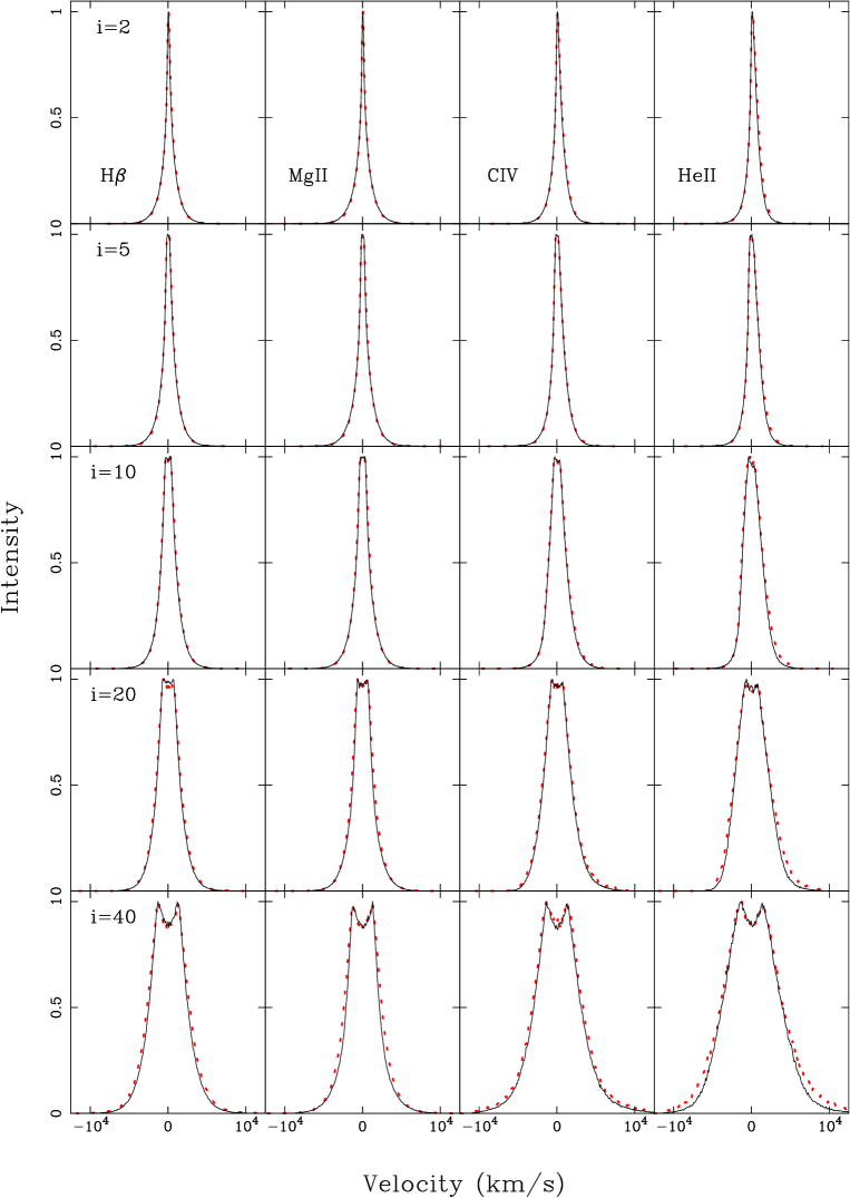
Figure 19: The corresponding variable emission-line profiles (solid black line) for figure 18. Shown in red is the equivalent variable line profile for emissivity-weighting only ($\eta(r)=constant$). All profiles have been normalised to their peak intensity to aid comparison.

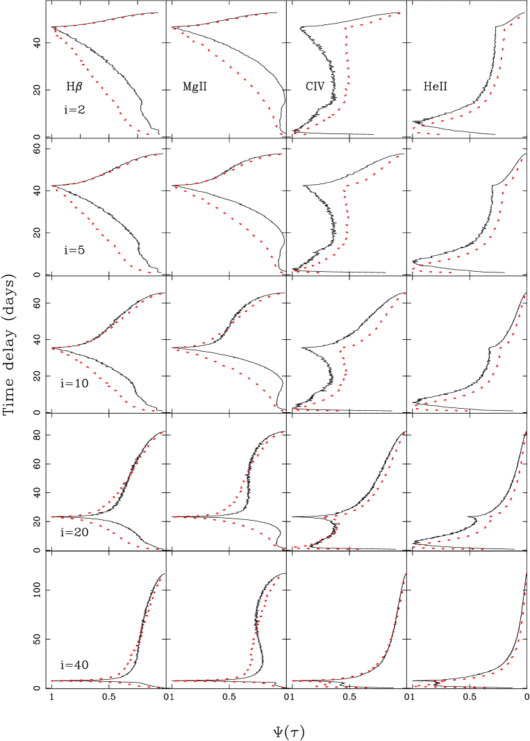
Figure 20: The corresponding 1-d responsivity-weighted response functions (solid black line) for figure 18. Shown in red is the equivalent emissivity-weighted (ie. $\eta(r)=constant$) 1-d response function. Response functions have been normalised to their peak intensities to aid comparison. Responsivity-weighting significantly modifies both the form and amplitude of the 1-d response.

Appendix B Anisotropic illumination

A strong assumption of our model is that the gas on the bowl-surface is illuminated by a continuum whose shape is independent of scale height. Yet, in the TOR model of Kawaguchi and Mori (2010,2011) the bowl-shaped geometry is formed because the disc emission is strongly anisotropic, thereby allowing dust grains to form at much smaller radii at low elevations (near to mid-plane of the disc). If an anisotropic continuum source is indeed responsible for shaping the bowl geometry, then it will almost certainly have a strong effect on the shape of the 1-d and 2-d responsivity-weighted response function and variable emission-line profile. Here we look at 3 alternative models for the disc continuum emission : strong, intermediate and weak anisotropy. For each we model the broad band continuum as the sum of a varying UV component and a constant X-ray component, the relative fractions of which are determined by the dependence of the intensity of the UV component on the polar angle.

To represent the strong anisotropy dependence we adopt the disc-illumination function first proposed by Netzer (1987), ie.

$$I(\phi)=\frac{I_{\rm uv}}{3}\cos\phi\left(1+2\cos\phi\right)+I_{\rm x}\,,$$ (7)

where $I_{uv}$ and $I_{x}$ are the relative intensities (or ionising photon fluxes) of the UV and X-ray components, and $\phi$ is the polar angle. The weak anisotropy function is taken from Nemmen and Brotherton (2010), for which we assume

$$I(\phi)=I_{\rm uv}\sin\left[\left(\frac{\pi}{2}\times\frac{\phi_{0}}{\phi}\right)^{10}\right]+I_{\rm x}\,,$$ (8)

for polar angles $\phi\geq\phi_{0}=72$ degrees, and

$$I(\phi)=I_{\rm uv}+I_{\rm x}\,,$$ (9)

otherwise. Finally, we model an intermediate anisotropic illumination function with a simple cosine dependence, ie.

$$I(\phi)=I_{\rm uv}\cos\phi+I_{\rm x}\,.$$ (10)

Note we do not calculate new photoionisation model grids for a broad range of continuum shapes. Instead as a first approximation, we assume that we can use our original emissivity grids (line flux as a function of radial distance $R$ and hydrogen ionising photon flux $\Phi_{\rm H}$) as a look-up table. That is we use the line flux at a given radial distance to find the corresponding hydrogen ionising photon flux $\Phi_{H}$. $\Phi_{\rm H}$ is then modified according to equations B1–B4, and a new flux determined from the same model grid. In figure 21 we illustrate the modified H$\beta$ radial emissivity distribution for each of the disc illumination functions. Figure 22 illustrates the 1-d responsivity-weighted response functions (upper panel) and variable emission-line profiles (lower panel) resulting from the modified radial emissivity distributions as described above for our fiducial model and $i=30$ degrees. For each model we assume that the UV continuum comprises 99% of the total ionising continuum intensity, ie. $I_{\rm uv}=0.99I_{\rm totl}$.

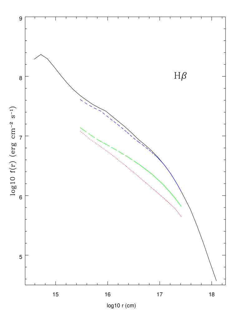
Figure 21: The radial surface line emissivity distributions for our disc illumination functions: Isotropic continuum – black solid line, Netzer’s disc illumination function – red dotted line, a disc illumination pattern approximating that of Nemmen and Brotherton (2010) – blue dashed line, and a disc illumination function with simple cosine dependence – green long-dashed line.

Figure 22: 1-d responsivity-weighted response functions and variable emission-line profiles for the disc illumination functions described in the text for our fiducial bowl-shape BLR geometry, turbulence parameter $b_{turb}=2$, and observed at inclination $i=30$ degrees. Isotropic continuum – solid line, Netzer’s disc illumination function – dotted line, a disc illumination pattern approximating that of Nemmen and Brotherton (2010) – dashed line (nearly coincident with the solid line), and a disc illumination function with a simple cosine dependence – long-dashed line.

Appendix C The driving continuum light-curve

The X-ray light curves of AGN show correlated variability over a broad range in timescales. This variability is normally quantified in terms of the variability power, $P$, as a function of temporal frequency $\nu$, the power spectral density (PSD) distribution. For AGN, the X-ray PSD is approximated by a power-law in frequency ($P\propto\nu^{-\alpha}$) with slope $\alpha=1$ at low frequencies, breaking to a slope of $2$ at the highest frequencies (McHardy et al. 2004) appropriate for a red-noise process.

At optical wavelengths, poor temporal sampling has often negated the use of the PSD in determining the optical continuum variability. Instead, variability is generally characterised in terms of the first order structure function $S(\tau)$ (Collier and Peterson 2001), where

$$S(\tau)=\frac{1}{N(\tau)}\sum_{i<j}[f(t_{i})-f(t_{j})]^{2}\,,$$ (11)

where $f$($t_{i}$) is the flux measured at time $t_{i}$, $N(\tau)$ is the number of pairs of points, and the sum is over all pairs for which $\tau=t_{j}-t_{i}$. Paltani (1999) showed that the first order structure function is related to the one-sided power density spectrum $P(f)$ via:

$$S(\tau)=2\left[\int_{0}^{\infty}P(f)df-\int_{0}^{\infty}\cos(2\pi f\tau)df\right]\,.$$ (12)

The form of the structure function can also be approximated by a power-law on intermediate timescales, breaking to a flatter slope on both short timescales ($\tau_{min}$), where its value approaches twice the noise variance ($\sigma_{n}^{2}$), and on long-timescales ($\tau_{max}$), where its value approaches twice the signal variance ($\sigma_{var}^{2}$).

Collier and Peterson (2001) performed a structure function analysis of the UV and optical light-curves of a small sample (13) of AGN, including NGC 5548, observed as part of the ’AGN Watch’ and OSU AGN monitoring programmes. They showed that the UV and optical SFs are similar on timescales of 5–60 days. In particular, for NGC 5548, the UV and optical power-law slope $b$ of the SF on intermediate timescales is approximately 1.5, and flattens on a characteristic timescale $\tau_{char}=40$ days. For stationary time series, the power-law slope of the structure function $b$ is related to the power-law slope of the PSD $\alpha$, by $\alpha=b+1$. Thus, for NGC 5548, the slope of the UV and optical SF suggests $\alpha\approx 2.5$. However, we caution that non-stationary effects can steepen the derived power-law slope while deviations from a strictly power-law slope may be introduced by bias resulting from binning and irregular sampling of the data (Collier and Peterson 2001). For a stationary random process $S(\tau)$ is simply related to the autocorrelation function $ACF(\tau$), such that

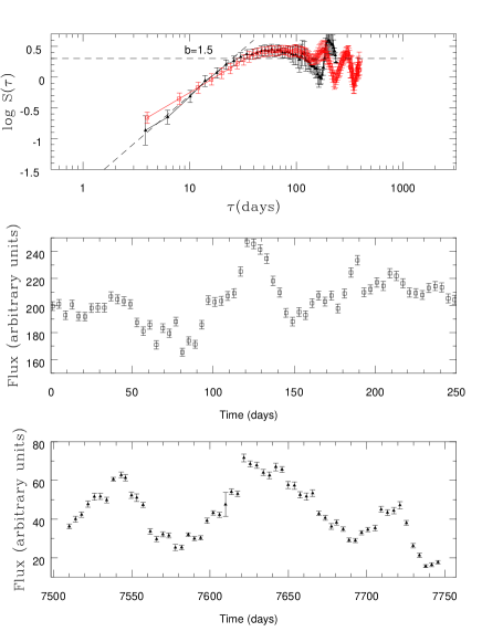
Figure 23: Upper panel – a typical structure function for one of our simulated light-curves (open squares). Also shown is the structure function derived for the GEX extracted 1337Åcontinuum from the 1989 IUE monitoring campaign of NGC 5548. Middle-panel – the corresponding simulated light-curve sampled at 4 day intervals. Lower-panel – the 1337Åcontinuum light-curve from the 1989 monitoring campaign of NGC 5548.

$$S(\tau)=2\left[\sigma^{2}-ACF(\tau)\right]\,\ .$$ (13)

Thus the form of the SF can vary from one observing season to the next even when the process responsible for the variability remains the same. Similar critiques have been made concerning the use of structure functions in quantifying Blazar variability (Emmanoulopoulos et al. 2010), and in particular when assigning characteristic timescales to features observed in the SF on long timescales where the SF is poorly defined.

In figure 23 (top panel) we indicate a typical structure function calculated from one of our model light-curves (open squares). Also shown is the structure function derived from the GEX extracted 1337Å continuum light-curve (filled triangles) of NGC 5548 taken from the 1989 IUE monitoring campaign (Clavel et al. 1991). The dashed diagonal line indicates the slope of the structure function over the region of interest. In the middle panel we show the simulated light-curve sampled at 4 day intervals (to match the sampling of the light-curve in the IUE campaign). The lower panel, shows the continuum light-curve from the 1989 IUE monitoring campaign.