Combining F-Term Hybrid Inflation With a Peccei-Quinn Phase Transition

Abstract:

We consider an inflationary model based only on renormalizable superpotential terms in which a superheavy scale F-term hybrid inflation (FHI) is followed by a Peccei-Quinn (PQ) phase transition. We show that the field which triggers the PQ phase transition influences drastically the inflationary dynamics and that the Universe undergoes a secondary phase of reheating after the PQ phase transition. Confronting FHI with the current observational data we find that, for the central value of the spectral index, the grand unification scale can assume its supersymmetric value for more or less natural values for the remaining model parameters. On the other hand, the final reheat temperature after the PQ phase transition turns out to be low enough to avoid the gravitino problem.

Published in  PoS (CORFU2011) 028.

1 Introduction

In this talk, which is based on Ref. [1], we describe how we can achieve a cosmological scenario in which a superheavy F-term hybrid inflation (FHI) is followed by a Peccei-Quinn phase transition (PQPT) using two similar renormalizable superpotential terms. Below, we first briefly review the basic ingredients of our construction in Sec. 1.1 and Sec. 1.2 and outline the structure of our proposal in Sec. 1.3.

1.1 F-term Hybrid Inflation

One of the most natural, popular and well-motivated inflationary model is the supersymmetric (SUSY) FHI [2, 3, 4]. It can be realized adopting the superpotential

$$W_{\rm FHI}=\kappa S\left(\bar{\Phi}\Phi-M^{2}\right),$$ (1)

which is consistent with a continuous $R$-symmetry [3] under which

$$S\ \to\ e^{i\alpha}\,S,~{}\bar{\Phi}\Phi\ \to\ \bar{\Phi}\Phi,~{}W_{\rm FHI}\to\ e^{i\alpha}\,W_{\rm FHI}.$$ (2)

Here, $S$ is a left-handed (LH) superfield, singlet under a grand unified theory (GUT) gauge group $G$; $\bar{\Phi}$ and $\Phi$ is a pair of LH superfields belonging to non-trivial conjugate representations of $G$, and reducing its rank by their vacuum expectation values (v.e.vs); $\kappa$ and $M$ are parameters which can be made positive by field redefinitions.

The SUSY potential induced by $W_{\rm FHI}$ in Eq. (1) along the D-flat direction $|\bar{\Phi}|=|\Phi|$ is

$$V_{\rm FHI}=\kappa^{2}\left|\bar{\Phi}\Phi-M^{2}\right|^{2}+\kappa^{2}|S|^{2}\left(|\bar{\Phi}|^{2}+|\Phi|^{2}\right).$$ (3)

$W_{\rm FHI}$ gives rise to FHI, since there is a F-flat direction, with $\bar{\Phi}=\Phi=0$ and constant potential energy $V_{\rm F}\simeq\kappa^{2}M^{4}$, which is a local minimum of $V_{\rm F}$ for $S>M$. Also, $W_{\rm FHI}$ leads to the spontaneous breaking of $G$, since the SUSY vacuum lies at

$$\langle S\rangle=0~{}~{}\mbox{and}~{}~{}|\langle\bar{\Phi}\rangle|=|\langle\Phi\rangle|=M,$$ (4)

with the non-zero v.e.vs of $\bar{\Phi}$ and $\Phi$ developed along the Standard Model (SM) singlet directions.

One of the shortcomings of FHI is the tension which, in general, exists between the predicted (scalar) spectral index $n_{\rm s}$ and the recent seven-year results [5] from the Wilkinson microwave anisotropy probe (WMAP7) satellite. Indeed, it is well-known that the realization of FHI within minimal Supergravity (SUGRA) leads to $n_{\rm s}$ which is just marginally consistent with the fitting of the WMAP7 data by the standard power-law cosmological model with cold dark matter and a cosmological constant ($\Lambda$CDM). One possible resolution of this problem is [6] the addition to the Kähler potential of a non-minimal quatric term of the inflaton field with a convenient choice of its sign. As a consequence, a negative mass term for the inflaton is generated. In the largest part of the parameter space, the inflationary potential acquires a local maximum and minimum. Then, FHI of the hilltop type [7] can occur as the inflaton rolls from this maximum down to smaller values. Therefore, $n_{\rm s}$ can become consistent with data, but only at the cost of an extra indispensable mild tuning [6] of the initial conditions. Another possible complication is that the system may get trapped near the minimum of the inflationary potential and, consequently, no FHI takes place.

1.2 Supersymmetrizing the PQ Solution to the Strong CP Problem

Due to the non-perturbative structure of the vacuum of $SU(3)_{\rm C}$ the lagrangian of quantum chromodynamics (QCD) includes a CP-violating term, involving the strong coupling constant, $g_{3}$, the gluon field-strength tensor, ${\mathcal{G}}$, and its dual, $\widetilde{\mathcal{G}}$. I.e.,

$${\cal L}_{\rm QCD}={g_{3}^{2}\over 32\pi^{2}}\bar{\theta}\ {\mathcal{G}}^{\rm a\mu\nu}\ \widetilde{\mathcal{G}}^{\rm a}_{\mu\nu}+\cdots~{}~{}\mbox{with}~{}~{}\bar{\theta}\lesssim 5\cdot 10^{-10},$$ (5)

since $\bar{\theta}$ is involved in the computation of the neutron electric dipole moment which is experimentally determined, with result

$$d_{\rm n}\simeq 4.5\cdot 10^{-16}\ \bar{\theta}<2.9\cdot 10^{-26}~{}\mbox{e-cm~{}~{}~{}at~{}~{}90\% c.l.}$$ (6)

The smallness of $\bar{\theta}$ consists the infamous strong CP problem. The most promising solution, proposed [8] by Peccei and Quinn, is to introduce a global color anomalous $U(1)_{\rm PQ}$ symmetry which is spontaneously broken at an energy scale $f_{a}\simeq(10^{9}-10^{12})~{}{\mbox{\rm GeV}}$, known as PQ energy scale. The Goldstone boson, $a(x)$, associated with such symmetry breaking is called axion. The Lagrangian term resulting after the spontaneous symmetry breaking of the $U(1)_{\rm PQ}$ symmetry reads:

$${\cal L}_{a}={1\over 2}\partial^{\mu}a\partial_{\mu}a+c_{a}{g_{3}^{2}\over 32\pi^{2}}{a\over f_{a}}{\mathcal{G}}^{\rm a}_{\mu\nu}\widetilde{\mathcal{G}}_{\rm a\mu\nu},$$ (7)

where $c_{a}$ is a model-dependent parameter. When considering the total lagrangian parts of Eqs. (5) and (7), an effective potential for $a$ appears, whose minimum is reached when the so-called (axion) misalignment angle vanishes, i.e.,

$$\theta=\bar{\theta}+c_{a}{a\over f_{a}}=0~{}~{}\mbox{or}~{}~{}<a>=-\bar{\theta}{f_{a}\over c_{a}}\>\cdot$$ (8)

Therefore, minimizing the potential with respect to $a$ sets the offending CP-violating term to zero. Essentially, $\bar{\theta}$ is promoted to a dynamical variable that evolves to its CP-conserving minimum, $\theta=0$, where $\theta$ can be seen as the phase of a new complex scalar field, named PQ field.

Within a SUSY framework, the spontaneous breaking of $U(1)_{\rm PQ}$ can be obviously realized adopting [9] a renormalizable superpotential, $W_{\rm PQ}$, similar to that of Eq. (1) where $S$ is replaced by another $G$ and PQ singlet LH superfield, $P$, with the same $R$ charge, while $\Phi$ and $\bar{\Phi}$ are replaced by a pair of $G$ singlet oppositely PQ-charged LH superfields, $\bar{Q}$ and $Q$. Indeed, the superpotential

$$W_{\rm PQ}=\kappa_{a}P\left(\bar{Q}Q-f_{a}^{2}/4\right),$$ (9)

is invariant under the $U(1)_{\rm PQ}$ transformations

$$P\ \to\ P,\>Q\ \to\ e^{i\alpha}\,Q,\bar{Q}\ \to\ e^{-i\alpha}\,Q$$ (10)

and lead to the F-term SUSY potential

$$V_{\rm PQF}=\kappa_{a}^{2}\left|\bar{Q}Q-f^{2}_{a}/4\right|^{2}\ +\ \kappa^{2}_{a}\left|P\right|^{2}\left(|\bar{Q}|^{2}+|Q|^{2}\right),$$ (11)

from where we can infer that $U(1)_{\rm PQ}$ can be spontaneously broken due to the following v.e.vs:

$$\langle{P}\rangle\simeq 0~{}~{}\mbox{and}~{}~{}\langle{\phi_{Q}}\rangle=f_{a}~{}~{}~{}\mbox{with}~{}~{}~{}2Q=2{\bar{Q}}=\phi_{Q}$$ (12)

– since the sum of the arguments of $\langle{\bar{Q}}\rangle$ and $\langle{Q}\rangle$ must be $0$, $\bar{Q}$ and $Q$ can be brought to the real axis by an appropriate PQ transformation. In reality, however, the total potential of the PQ fields is

$$V_{{\rm PQ}a}=V_{\rm PQF}+V_{a},~{}~{}~{}\mbox{where}~{}~{}~{}V_{a}=m^{2}_{a}(T)f_{a}^{2}(1-\cos\theta)$$ (13)

(with $m_{a}$ the temperature, $T$, dependent $a$ mass) comes from nonperturbative QCD effects associated with instantons [10], that break explicitly $U(1)_{\rm PQ}$ down to a $\mathbb{Z}_{N}$ discrete subgroup, where $N$ is the sum of the PQ charges of the $SU(3)_{\rm C}$ triplets and antitriplets of the model. Therefore, the breakdown of $\mathbb{Z}_{N}$ by the v.e.vs in Eq. (12) may lead [10] to cosmologically catastrophic domain walls which, however, can be avoided [11] by introducing extra matter superfields – see Sec. 2.3.

A by-product of the $U(1)_{\rm PQ}$ spontaneous breaking is that we can achieve [12] a resolution of the $\mu$-problem of MSSM by considering, e.g., a non-renormalizable superpotential term of the form $\bar{Q}^{2}H_{u}H_{d}/m_{\rm P}$, which after the spontaneous breakdown of $U(1)_{\rm PQ}$ leads to the $\mu$ term of the MSSM, with $|\mu|\sim\lambda_{\mu}\left|\langle{\bar{Q}}\rangle\right|^{2}/m_{\rm P}$, which is of the right magnitude if $\left|\langle{\bar{Q}}\rangle\right|=f_{a}/2\simeq 5\cdot 10^{11}~{}{\rm GeV}$ and $\lambda_{\mu}\simeq(0.001-0.01)$ – here, $m_{\rm P}\simeq 2.44\cdot 10^{18}~{}{\rm GeV}$ is the reduced Planck scale; $H_{u}$ and $H_{d}$ are the electroweak Higgses of MSSM which couple to up- and down-type quarks respectively.

1.3 Outline

The key point of our attempt in combining both ingredients (FHI and PQPT) described in Sec. 1.1 and 1.2 is that $P$ can be regarded as the linear combination of the $G\times U(1)_{\rm PQ}$ singlets with the $R$ charge of the superpotential that does not couple to $\bar{\Phi}\Phi$ – cf. Ref. [13]. As a consequence, an unavoidable superpotential coupling $S\bar{Q}Q$ and a $S-P$ mixing in the Kähler potential arise – see Sec. 2. These facts influence drastically the inflationary set-up described in Sec. 3. In addition, the value of $P$ after FHI is to be kept larger than $f_{a}/2$ so as to achieve an instantaneous domination of the PQ system over radiation in order to alleviate the gravitino ($\widetilde{G}$) problem [14, 15]. These effects are presented in Sec. 4. We end up testing our model against observations in Sec. 5 and summarizing our results in Sec. 6.

2 Model Description

We below describe the structure of our model in Sec. 2.1, we sketch its cosmological consequences in Sec. 2.2 and explain how we avoid the formation of domain walls in Sec. 2.3.

2.1 The General Set-up

In order to explore our scenario, we identify $G$ with the left-right symmetric gauge group $G_{\rm LR}=SU(3)_{\rm C}\times SU(2)_{\rm L}\times SU(2)_{\rm R}\times U(1)_{B-L}$, which can be broken down to the SM gauge group $G_{\rm SM}=SU(3)_{\rm C}\times SU(2)_{\rm L}\times U(1)_{Y}$ through the v.e.vs acquired by a conjugate pair of $SU(2)_{\rm R}$ doublet Higgs, $\bar{\Phi}$ and $\Phi$. As a consequence, no cosmic strings are produced in the end of FHI and, therefore, no extra restrictions on the parameters have to be imposed – c.f. Ref. [16]. The model possesses also three global $U(1)$ symmetries. Namely, a (color) anomalous $R$ symmetry ${U(1)_{R}}$, an anomalous PQ symmetry ${U(1)}_{\rm PQ}$ and the baryon number symmetry ${U(1)}_{B}$. The representations under $G_{\rm LR}$ and the charges under the global symmetries of the various matter and Higgs superfields are presented in Table 1, which also contains $n$ extra matter superfields ($\bar{D}_{\rm a}-D_{\rm a}$ and $H_{\rm a}$) required for evading the domain-wall problem associated with PQPT together with a new imposed global ${U(1)}_{D}$ symmetry – see Sec. 2.3.

Super-	Represen-	Transfor-	Decom-	Global
fields	tations	mations	positions	Symmetries
	under $G_{\rm LR}$	under $G_{\rm LR}$	under $G_{\rm SM}$	$R$	PQ	$B$	$D$
Matter Fields
$l_{i}$	$({\bf 1,2,1},-1)$	$l_{i}U_{\rm L}^{\mbox{\sf\scriptsize T}}$	$l_{i}({\bf 1,2},-1/2)$	$0$	$-2$	$0$	$0$
$l^{c}_{i}$	$({\bf 1,1,2},1)$	$U_{\rm R}^{\ast}l^{c}_{i}$	$\nu_{i}^{c}({\bf 1,1},0)$	$2$	$0$	$0$	$0$
			$e_{i}^{c}({\bf 1,1},1)$
$q_{i}$	$({\bf 3,2,1},1/3)$	$q_{i}U_{\rm L}^{\mbox{\sf\scriptsize T}}\ U_{\rm C}^{\mbox{\sf\scriptsize T}}$	$q_{i}({\bf 3,2},1/6)$	$1$	$-1$	$1/3$	$0$
$q^{c}_{i}$	$({\bf\bar{3},1,2},-1/3)$	$U_{\rm C}^{\ast}\ U_{\rm R}^{\ast}q^{c}_{i}$	$u^{c}_{i}({\bf\bar{3},1},-2/3)$	$1$	$-1$	$-1/3$	$0$
			$d_{i}^{c}({\bf\bar{3},1},1/3)$
Extra Matter Fields
$\bar{D}_{\rm a}$	$({\bf\bar{3},1,1},2/3)$	$U_{\rm C}^{\ast}D_{\rm a}$	$\bar{D}_{\rm a}({\bf\bar{3},1},-1/3)$	$2$	$1$	$0$	$-1$
$D_{\rm a}$	$({\bf 3,1,1},-2/3)$	$D_{\rm a}U_{\rm C}^{\mbox{\sf\scriptsize T}}$	$D_{\rm a}({\bf 3,1},1/3)$	$2$	$1$	$0$	$1$
$H_{\rm a}$	$({\bf 1,2,2},0)$	$U_{\rm L}H_{\rm a}U_{\rm R}^{\mbox{\sf\scriptsize T}}$	$h_{\rm a}({\bf 1,2},1/2)$	$2$	$1$	$0$	$0$
			$\bar{h}_{\rm a}({\bf 1,2},-1/2)$
Higgs Fields
$S$	$({\bf 1,1,1},0)$	$S$	$S~{}({\bf 1,1},0)$	$4$	$0$	$0$	$0$
$\bar{\Phi}$	$({\bf 1,1,2},-1)$	$\bar{\Phi}U_{\rm R}^{\mbox{\sf\scriptsize T}}$	$\bar{\nu}_{\Phi}^{c}({\bf 1,1},0)$	$0$	$0$	$0$	$0$
			$\bar{e}^{c}_{\Phi}~{}({\bf 1,1},-1)$
$\Phi$	$({\bf 1,1,2},1)$	$U_{\rm R}^{\ast}\Phi$	$\nu_{\Phi}^{c}({\bf 1,1},0)$	$0$	$0$	$0$	$0$
			$e^{c}_{\Phi}~{}({\bf 1,1},1)$
$P$	$({\bf 1,1,1},0)$	$P$	$P~{}({\bf 1,1},0)$	$4$	$0$	$0$	$0$
$\bar{Q}$	$({\bf 1,1,1},0)$	$\bar{Q}$	$\bar{Q}~{}({\bf 1,1},0)$	$0$	$-2$	$0$	$0$
$Q$	$({\bf 1,1,1},0)$	$Q$	$Q~{}({\bf 1,1},0)$	$0$	$2$	$0$	$0$
$h$	$({\bf 1,2,2},0)$	$U_{\rm L}hU_{\rm R}^{\mbox{\sf\scriptsize T}}$	$H_{u}~{}({\bf 1,2},1/2)$	$2$	$2$	$0$	$0$
			$H_{d}~{}({\bf 1,2},-1/2)$

Table 1: The representations, the transformations under $G_{\rm LR}$, the decompositions under $G_{\rm SM}$ as well as the extra global charges of the superfields of our model. Here, $U_{\rm C}\in SU(3)_{\rm C},~{}U_{\rm L}\in SU(2)_{\rm L},~{}U_{\rm R}\in SU(2)_{\rm R}$ and T and $\ast$ stand for the transpose and the complex conjugate of a matrix respectively.

In particular, the superpotential, $W$, of our model reads:

$$W=W_{\rm FHI}+W_{\rm PQ}+\lambda S\bar{Q}Q\ +\ W_{\rm MSSM}+W_{\rm DW},$$ (14)

where $W_{\rm FHI}$ and $W_{\rm PQ}$ are given by Eqs. (1) and (9) respectively and the anticipated in Sec. 1.3 unavoidable coupling is included. In addition,

$\bullet$ $W_{\rm MSSM}$ is the part of $W$ which contains the usual terms of the Minimal SUSY SM (MSSM), supplemented by a mass term and Yukawa interactions for right-handed neutrinos, $\nu^{c}_{i}$:

$$W_{\rm MSSM}=\lambda_{\mu}{\bar{Q}^{2}h^{2}\over 2m_{\rm P}}+y_{\nu ij}{\bar{\Phi}l^{c}_{i}\bar{\Phi}l^{c}_{j}\over m_{\rm P}}+y_{lij}l_{i}hl^{c}_{j}+y_{qij}q_{i}hq^{c}_{j}\>.$$ (15)

Here, the $i$th generation $SU(2)_{\rm L}$ doublet LH quarks and leptons are denoted by $q_{i}$ and $l_{i}$ respectively, whereas the $SU(2)_{\rm R}$ doublet antiquarks and antileptons by $q^{c}_{i}$ and $l^{c}_{i}$ respectively. The electroweak Higgs are contained in a $SU(2)_{\rm L}\times SU(2)_{\rm R}$ bidoublet Higgs $h$. The first term in the right-hand side (RHS) of Eq. (15) generates the $\mu$ term of MSSM via the PQ breaking scale – see Sec. 1.2 –, while the second term generates intermediate scale masses for $\nu^{c}_{i}$ and, thus, seesaw masses [3] for the light neutrinos – the coupling constant matrix $y_{\nu ij}$ is considered diagonal.

$\bullet$ $W_{\rm DW}$ is the part of $W$ which gives intermediate scale masses via $\langle{\bar{Q}}\rangle$ – see Sec. 1.2 – to $\bar{D}_{\rm a}-D_{\rm a}$ and $H_{\rm a}$. Namely,

$$W_{\rm DW}=\lambda_{D\rm a}\bar{Q}\bar{D}_{\rm a}D_{\rm a}+\lambda_{H\rm a}\bar{Q}H_{\rm a}^{2},$$ (16)

where the coupling constant matrices $\lambda_{D\rm a}$ and $\lambda_{h\rm a}$ are considered diagonal. Although these matter fields acquire intermediate scale masses after the PQ breaking, the unification of the MSSM gauge coupling constants is not disrupted at one loop. In fact, if we estimate the contribution of $\bar{D}_{\rm a},D_{\rm a},$ and $\bar{H}_{\rm a}$ to the coefficients $b_{1},~{}b_{2},$ and $b_{3}$, controlling [17] the one loop evolution of the three gauge coupling constants $g_{1},g_{2},$ and $g_{3}$, we find that the quantities $b_{2}-b_{1}$ and $b_{3}-b_{2}$ (which are [17] crucial for the unification of $g_{1},g_{2},$ and $g_{3}$) remain unaltered.

The Kähler potential for our model can include interference terms of $S$ and $P$ even at the quadratic level, i.e., it has the form

$$K = |S|^{2}+|P|^{2}+{\mbox{\sl a}}(SP^{*}+S^{*}P)+b{|S|^{4}\over 4m_{\rm P}^{2}}+c{|P|^{4}\over 4m_{\rm P}^{2}}+d{|S|^{2}|P|^{2}\over m_{\rm P}^{2}}+\ {e|S|^{2}+f|P|^{2}\over 2m_{\rm P}^{2}}\left(SP^{*}+S^{*}P\right)$$ (17)

$$+ \ {{\rm g}\over 4m_{\rm P}^{2}}\left[\left(SP^{*}\right)^{2}+\left(S^{*}P\right)^{2}\right]+\ \cdots,$$

where all the coefficients ${\mbox{\sl a}},b,c,d,e,f$ and ${\rm g}$ are taken, for simplicity, real. The ellipsis represents terms involving the waterfall fields ($\Phi$, $\bar{\Phi}$, $Q$, and $\bar{Q}$) which have negligible impact on our analysis.

2.2 The Cosmological Scenario

The F–term SUGRA scalar potential, $V_{\rm SUGRA}$ of our model can be found by applying the well-known formula – see e.g. Ref. [2]:

$$V_{\rm SUGRA}=e^{K/m_{\rm P}^{2}}\left(F_{i^{*}}^{*}\left(K_{,ji^{*}}\right)^{-1}F_{j}-3\frac{|W|^{2}}{m_{\rm P}^{2}}\right)~{}~{}\mbox{with}~{}~{}F_{i}=W_{,i}+K_{,i}{W\over m_{\rm P}^{2}}\cdot$$ (18)

Here, a subscript $,i~{}[,i^{*}]$ denotes derivation with respect to the complex scalar field $i~{}[i\,^{*}]$. Taking the limit $m_{\rm P}\to\infty$, we can obtain the SUSY limit of $V_{\rm SUGRA}$, $V_{\rm F}$, which turns out to be

$$V_{\rm F} = {1\over(1-{\mbox{\sl a}}^{2})}\left(\left|\kappa\left(\bar{\Phi}\Phi-M^{2}\right)+\lambda\bar{Q}Q\right|^{2}+\ \kappa_{a}^{2}\left|\bar{Q}Q-M^{2}_{a}\right|^{2}\right)+\ \kappa^{2}|S|^{2}\left(|\bar{\Phi}|^{2}+|\Phi|^{2}\right)$$ (19)

$$+ \left|\lambda SQ+\kappa_{a}PQ+\lambda_{D\rm a}\bar{D}_{\rm a}D_{\rm a}+\lambda_{H\rm a}H_{\rm a}^{2}\right|^{2}+\ |\bar{Q}|^{2}\left(\left|\lambda S+\kappa_{a}P\right|^{2}+\lambda_{D\rm a}^{2}\left(|\bar{D}_{\rm a}|^{2}+|D_{\rm a}|^{2}\right)+\lambda_{H\rm a}^{2}|H_{\rm a}|^{2}\right)$$

$$- {{\mbox{\sl a}}\over(1-{\mbox{\sl a}}^{2})}\Big{[}{\kappa_{a}}\left(\bar{Q}^{*}Q^{*}-M^{2}_{a}\right)\big{[}\kappa\left(\bar{\Phi}\Phi-M^{2}\right)+\ \lambda\bar{Q}Q\big{]}+\mbox{c.c.}\Big{]},$$

where the complex scalar components of the superfields are denoted by the same symbol. From the potential in Eq. (19) and taking into account that $M\gg f_{a}$, we find that the SUSY vacuum lies at the directions – cf. Eqs. (4) and (12):

$$\langle{S}\rangle\simeq 0,~{}\langle{P}\rangle\simeq 0,~{}\langle{\bar{D}_{a}}\rangle=\langle{D_{a}}\rangle=\langle{H_{a}}\rangle=\langle{\bar{e}^{c}_{\Phi}}\rangle=\langle{e^{c}_{\Phi}}\rangle=0,$$ (20a)

$$\langle{\bar{\nu}^{c}_{\Phi}}\rangle=\langle{\nu^{c}_{\Phi}}\rangle=M~{}~{}\mbox{and}~{}~{}\langle{\phi_{Q}}\rangle={f_{a}}\>,$$ (20b)

where we have introduced the canonically normalized scalar field $\phi_{Q}=2Q=2\bar{Q}$ – cf. Eq. (12). As a consequence, $W$ leads to a spontaneous breaking of $G_{\rm LR}$ and ${U}(1)_{\rm PQ}$. In addition, $W$ gives rise to a stage of FHI and a PQPT, since $V_{\rm F}$ possesses two D– and F–flat directions for

$$~{}\bar{\nu}^{c}_{\Phi}=\nu^{c}_{\Phi}=\bar{e}^{c}_{\Phi}=e^{c}_{\Phi}=\bar{Q}=Q=\bar{D}_{a}=D_{a}=H_{a}=0$$ (21a)

and $$~{}S=\bar{e}^{c}_{\Phi}=e^{c}_{\Phi}=\bar{Q}=Q=0~{}~{}\mbox{and}~{}~{}\bar{\nu}^{c}_{\Phi}=\nu^{c}_{\Phi}=M,$$ (21b)

with a constant potential energy density respectively

$${\footnotesize\sf(a)}~{}~{}V_{\rm HI0}\simeq{\kappa^{2}M^{4}}/{(1-{\mbox{\sl a}}^{2})}~{}~{}~{}~{}\mbox{and}~{}~{}~{}~{}{\footnotesize\sf(b)}~{}~{}V_{\rm PQ0}=\kappa_{a}^{2}f_{a}^{4}/16.$$ (22)

By constructing the scalar spectrum along the direction of Eq. (21a) – see Table 2 –, we can deduce that it can be used as inflationary path since it corresponds to a classically flat valley of minima for

$${\sf(a)}~{}~{}|S|>{M\over\sqrt{1-{\mbox{\sl a}}^{2}}}~{}~{}~{}\mbox{and}~{}~{}~{}{\sf(b)}~{}~{}|\sigma_{a}|>{\sqrt{\kappa(\lambda-{\mbox{\sl a}}\kappa_{a})\over 1-{\mbox{\sl a}}^{2}}}M,~{}~{}\mbox{where}~{}~{}\sigma_{a}=\lambda S+\kappa_{a}P.$$ (23)

Since $V_{\rm PQ0}\ll V_{\rm HI0}$, $V_{\rm PQ0}$ can dominate over radiation after the end of FHI leading to a PQPT. This cosmological scenario can be attained if Eq. (23a) is violated before Eq. (23b), since, in this case, we obtain $\bar{\nu}^{c}_{\Phi}=\nu^{c}_{\Phi}=M~{}\mbox{and}~{}\bar{Q}=Q=0$ and not $\bar{\nu}^{c}_{\Phi}=\nu^{c}_{\Phi}=0~{}\mbox{and}~{}\bar{Q}=Q=f_{a}/2$.

Super-	Scalars	Mass	Fermions	Mass
fields	(12 real)	Squared	(6 Weyl)	Squared
$\bar{\Phi}$, $\Phi$	${\mbox{\sf\footnotesize Re}}\ \&\ {\mbox{\sf\footnotesize Im}}~{}[\bar{\nu}^{c}_{\Phi}\pm\nu^{c}_{\Phi}]$	$\kappa^{2}\left(|S|^{2}\pm\frac{M^{2}}{1-{\mbox{\footnotesize\sl a}}^{2}}\right)$	$\psi_{\nu\pm}={\psi_{\bar{\nu}}\pm\psi_{\nu}\over\sqrt{2}}$	$\kappa^{2}|S|^{2}$
	${\mbox{\sf\footnotesize Re}}\ \&\ {\mbox{\sf\footnotesize Im}}~{}[\bar{e}^{c}_{\Phi}\pm e^{c}_{\Phi}]$		${\psi_{\bar{e}}\pm\psi_{e}\over\sqrt{2}}$
$\bar{Q}$, $Q$	${\mbox{\sf\footnotesize Re}}\ \&\ {\mbox{\sf\footnotesize Im}}~{}[\bar{Q}\pm Q]$	$|\sigma_{a}|^{2}\pm\frac{\kappa(\lambda-{\mbox{\footnotesize\sl a}}\kappa_{a})M^{2}}{1-{\mbox{\footnotesize\sl a}}^{2}}$	$\psi_{Q\pm}={\psi_{\bar{Q}}\pm\psi_{Q}\over\sqrt{2}}$	$|\sigma_{a}|^{2}$

Table 2: The SUSY-breaking mass spectrum along the inflationary trajectory of Eq. (2.8a). Here, $\psi_{x}$ with $x=\bar{\nu},\nu,\bar{e},e,\bar{Q}$ and $Q$ denote the chiral fermions associated with the superfields $x=\bar{\nu}^{c}_{\Phi},\nu^{c}_{\Phi},\bar{e}^{c}_{\Phi},e^{c}_{\Phi},\bar{Q}$ and $Q$ respectively.

2.3 Evading the Domain-Wall Problem

Soft SUSY breaking and instanton effects explicitly break ${U(1)_{R}}\times{U(1)_{\rm PQ}}$ to a discrete subgroup, which can be found, for every $n$, by solving the system of equations:

$$\left.\begin{matrix}e^{irR(W)}=1\hfill\cr e^{ir\sum_{i}R(i)+p\sum_{i}PQ(i)}=1\hfill\cr\end{matrix}\right\}\Rightarrow\left\{\begin{matrix}4r=0~{}\left(\mbox{\footnotesize\sf mod}~{}2\pi\right)\hfill\cr-12r+2(n-6)p=0~{}\left(\mbox{\footnotesize\sf mod}~{}2\pi\right)\hfill\cr\end{matrix}\right.~{}~{}\mbox{where}~{}~{}\left\{\begin{matrix}e^{irR}\in U(1)_{R}\hfill\cr e^{ipPQ}\in U(1)_{\rm PQ},\hfill\cr\end{matrix}\right.$$ (24)

with $r$ [$p$] being a $U(1)_{R}$ [$U(1)_{\rm PQ}$] rotation and the sum over $i$ is applied over all ${SU(3)_{\rm C}}$ ${\bf 3}$ and ${\bf\bar{3}}$ of the model. We conclude that the unbroken subgroup is $\mathbb{Z}_{4}\times\mathbb{Z}_{2(n-6)}$. It is then important to ensure that this subgroup is not spontaneously broken by $\langle{Q}\rangle$ and $\langle{\bar{Q}}\rangle$, i.e., the equations

$$e^{2ip_{s}}\langle{Q}\rangle=\langle{Q}\rangle~{}~{}\mbox{and}~{}~{}e^{-2ip_{s}}\langle{\bar{Q}}\rangle=\langle{\bar{Q}}\rangle~{}~{}\Rightarrow~{}~{}2p_{s}=0~{}\left(\mbox{\footnotesize\sf mod}~{}2\pi\right).$$ (25)

are satisfied identically – otherwise, cosmologically disastrous domain walls are produced [10] at PQPT. This goal can be accomplished by choosing $n=5$ or $n=7$. Therefore, for these $n$’s, the domain-wall production during PQPT can be eluded.

3 The Inflationary Era

Below, we describe the salient features of the inflationary potential in Sec. 3.1 and we analyze the inflationary dynamics in Sec. 3.2.

3.1 The Inflationary Potential

The inflationary potential along the trajectory of Eq. (21a) can be written as

$$V_{\rm HI}=V_{\rm HI0}+V_{\rm HIs}+V_{\rm HIc},~{}~{}\mbox{where}$$ (26)

$\bullet$ $V_{\rm HI0}$ is the dominant contribution to $V_{\rm HI}$ along the F-flat direction, given in Eq. (22a).

$\bullet$ $V_{\rm HIs}$ is the SUGRA corrections to $V_{\rm HI}$ which can be found by expanding $V_{\rm SUGRA}$ in Eq. (18) along the trajectory of Eq. (21a). Namely,

$$V_{{\rm HIs}} \simeq {V_{\rm HI0}\over(1-{\mbox{\sl a}}^{2})m^{2}_{\rm P}}\Big{[}A_{1}|S|^{2}+A_{12}\left(S^{*}P+PS^{*}\right)+A_{2}|P|^{2}\Big{]}+{V_{\rm HI0}\over 4(1-{\mbox{\sl a}}^{2})^{2}m^{4}_{\rm P}}\Big{[}B_{1}|S|^{4}+B_{2}|P|^{4}$$ (27a)

$$+ \ B_{3}|S|^{2}|P|^{2}+\left(B_{4}|S|^{2}+B_{5}|P|^{2}\right)\left(S^{*}P+PS^{*}\right)+B_{6}\left(\left(S^{*}P\right)^{2}+\left(P^{*}S\right)^{2}\right)\Big{]}$$

$$= {V_{\rm HI0}\over 2m_{\rm P}^{2}}\left(m^{2}_{+}\left(s^{2}+q^{2}\right)+m^{2}_{-}\sigma^{2}\right)+\cdots,\>\>$$

where the coefficients $$A_{1}-A_{3} B_{1}-B_{6} {\mbox{\sl a}},...,{\rm g} \sigma,s q m^{2}_{\pm} V_{\rm HIs} K_{SP} K$$ and , given in Ref. [1], are functions of the coefficients in Eq. (17); the real fields and are the eigenvectors (corresponding to the eigenvalues ) of the matrix involved in the quadratic part of . This can be worked out [1] after the quadratic part, , of in Eq. (17) has been brought into a canonical form, i.e., we obtain also

$$K_{SP}=|S|^{2}+|P|^{2}+{\mbox{\sl a}}(SP^{*}+S^{*}P)=\left(\sigma^{2}+s^{2}+q^{2}\right)/2.$$

Since $$m^{2}_{-}\simeq 0 \sigma K m^{2}_{-}\leq 0 n_{\rm s} {\mbox{\sl a}}\neq 0 b=c=d=e=f={\rm g}=0 m^{2}_{-}=0$$, its corresponding eigenvector, , can be qualified as the inflaton. Note that we need the higher order terms of in Eq. (17) so that we obtain and therefore, observationally acceptable ’s – see Sec. 5. Indeed, for and we get .

$\bullet$ $V_{\rm HIc}$ represents the contribution to $V_{\rm HI}$ from one-loop radiative corrections, due to SUSY-breaking mass spectrum presented in Table 2, which can be calculated [18] to be

$$V_{\rm HIc}\simeq{\kappa^{2}V_{\rm HI0}\over 8\pi^{2}(1-{\mbox{\sl a}}^{2})}\left(\ln{\kappa^{2}xM^{2}\over(1-{\mbox{\sl a}}^{2})\Lambda^{2}}+{3\over 2}\right)+{(\lambda-{\mbox{\sl a}}\kappa_{a})^{2}V_{\rm HI0}\over 16\pi^{2}(1-{\mbox{\sl a}}^{2})}\left(\ln{\kappa(\lambda-{\mbox{\sl a}}\kappa_{a})x_{a}M^{2}\over(1-{\mbox{\sl a}}^{2})\Lambda^{2}}+{3\over 2}\right)~{},$$ (27b)

with $x=|S|^{2}(1-{\mbox{\sl a}}^{2})/M^{2}$ and $x_{a}=|\sigma_{a}|^{2}(1-{\mbox{\sl a}}^{2})/\kappa(\lambda-{\mbox{\sl a}}\kappa_{a})M^{2}$. Here, we take into account that the dimensionality of the representations to which $\bar{\Phi}$ and $\Phi$ [$\bar{Q}$ and $Q$] belong is 2 [1] – see Table 1.

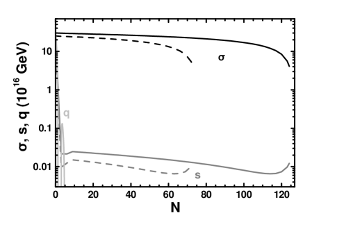
Figure 1: The evolution of $\sigma$ (black lines), $s$ (gray lines), and $q$ (light gray lines) as functions of $N$ for the values of the parameters shown in Eq. (5.4), $\kappa=0.0023,~{}{\mbox{\sl a}}=-0.011,~{}b=-0.01$ and $f_{\rm HIi}=3\cdot 10^{17}~{}{\mbox{\rm GeV}}$ (solid lines) or $f_{\rm HIi}=2.5\cdot 10^{17}~{}{\mbox{\rm GeV}}$ (dashed lines). For the employed values of parameters, the requirements of Sec. 5.1 are fulfilled.

3.2 The Inflationary Dynamics

The equations of motion (e.o.m) of the various fields are ($~{}~{}\dot{}=d/dt$ with $t$ the cosmic time):

$$\ddot{f}+3H\dot{f}+V_{{\rm HI},f}=0~{}\Rightarrow~{}H^{2}f^{\prime\prime}+3H^{2}f^{\prime}+V_{{\rm HI},f}=0~{}~{}\mbox{with}~{}~{}f=\sigma,~{}s,~{}\mbox{and}~{}q~{}$$ (28)

and ${}^{\prime}=d/dN$ where $N=\ln\left(R/R_{\rm HIi}\right)$. Here $R(t)$ is the scale factor of the universe and the subscript “HIi” denotes values at the onset of FHI. We impose the following initial conditions (at $N=0$):

$$f_{\rm HIi}=f(0)=(1.5-4.5)\cdot 10^{17}~{}{\mbox{\rm GeV}}~{}~{}\mbox{and}~{}~{}f^{\prime}(0)=0~{}~{}\mbox{with}~{}~{}f=\sigma,~{}s,~{}\mbox{or}~{}q.$$ (29)

When $f_{\rm HIi}$ is large enough, $s$ reaches an attractor and our results are independent of the precise value of $f_{\rm HIi}$, as can be clearly deduced from Fig. 1, where we plot $\sigma$ (black lines), $s$ (gray lines), and $q$ (light gray lines) as functions of $N$ for $f_{\rm HIi}=3\cdot 10^{17}~{}{\mbox{\rm GeV}}$ (solid lines) or $f_{\rm HIi}=2.5\cdot 10^{17}~{}{\mbox{\rm GeV}}$ (dashed lines). In both cases, we adopt the values of the parameters shown in Eq. (45), $\kappa=0.0045,~{}b=-0.01$ and ${\mbox{\sl a}}=-0.011$ which fulfill the requirements of Sec. 5.1. For both choices of $f_{\rm HIi}$’s, we obtain $m_{-}^{2}=-0.0126$, $m_{+}^{2}=1.83$, $n_{\rm s}=0.968$, $N_{\rm HI*}=52$, $\sigma_{\rm HIf}=4.08\cdot 10^{16}~{}{\mbox{\rm GeV}}$ and $s_{\rm HIf}=1.3\cdot 10^{14}~{}{\mbox{\rm GeV}}$ although in the first [second] case we obtain $N_{\rm HI}=87.1$ [$N_{\rm HI}=175.5$] – $N_{\rm HI}$ and $N_{\rm HI*}$ are defined below Eq. (38) in Sec. 5.1. We observe that immediately after the onset of FHI, $q$ decreases sharply, whereas the value of $s$ at the end of FHI, $s_{\rm HIf}$, turns out to be just mildly, and not drastically reduced compared to $\sigma$ – in sharp contrast to the situation of Ref. [19]. This is due to the participation of $s$ in both Eqs. (27a) and (27b).

4 The Post-Inflationary Era

We below describe the post-inflationary evolution of our model, presenting the dynamics of the two fields, $\sigma$ and $s$, in Sec. 4.1 and this of the two reheating processes in Sec. 4.2. For later convenience, we arrange in Table 3 the mass spectrum of our model at the SUSY vacuum of Eqs. (20a) and (20b).

Eigenstates		Eigenvalues	Eigenstates		Eigenvalues
Bosons	Fermions	(Masses)	Bosons	Fermions	(Masses)
$S,{\delta\bar{\nu}^{c}_{\Phi}+\delta\nu^{c}_{\Phi}\over\sqrt{2}}$	${\psi_{S}\pm\psi_{\nu+}\over\sqrt{2}}$	$m_{\rm I}=\sqrt{2}\kappa M$	$P,{\delta\bar{Q}+\delta Q\over\sqrt{2}}$	${\psi_{P}\pm\psi_{Q+}\over\sqrt{2}}$	$m_{\rm PQ}=\lambda_{a}{f_{a}\over\sqrt{2}}$
${\mbox{\sf\footnotesize Re}}[\bar{\nu}^{c}_{\Phi}-\nu^{c}_{\Phi}]$	${\psi_{\bar{\nu}}-\psi_{\nu}\over\sqrt{2}}$	$\sqrt{5/2}gM$	${\delta\bar{Q}-\delta Q\over\sqrt{2}}$	${\psi_{\bar{Q}}-\psi_{Q}\over\sqrt{2}}$	$0$
$\begin{matrix}{\mbox{\sf\footnotesize Re}}[\bar{e}^{c}_{\Phi}-e^{c}_{\Phi}]\cr{\sf\footnotesize Im}{\footnotesize[\bar{e}^{c}_{\Phi}+e^{c}_{\Phi}]}\cr\end{matrix}$	$\psi_{e},\psi_{\bar{e}}$	$gM$	$\tilde{\nu}^{c}_{i}$	$\nu^{c}_{i}$	$2y_{\nu i}M^{2}/m_{\rm P}$
${A^{1}_{\rm R}\pm iA^{2}_{\rm R}\over\sqrt{2}}$	${\uplambda^{1}_{\rm R}\pm i\uplambda^{2}_{\rm R}\over\sqrt{2}}$	$gM$	$D_{{\rm a}},~{}\bar{D}_{{\rm a}}$	$\psi_{D_{{\rm a}}},~{}\psi_{\bar{D}_{{\rm a}}}$	$\lambda_{D{\rm a}}f_{a}/2$
${A^{3}_{\rm R}\pm A_{B-L}\over\sqrt{2}}$	${\uplambda^{3}_{\rm R}\pm\uplambda_{B-L}\over\sqrt{2}}$	$0,\sqrt{5/2}gM$	$H_{{\rm a}}$	$\psi_{H_{{\rm a}}}$	$\lambda_{H{\rm a}}f_{a}/2$

Table 3: The mass spectrum of the model at the SUSY vacuum of Eq. (2.7a) and (2.7b). Here, $A_{\rm R}^{m}$ $[\uplambda_{\rm R}^{m}]$ with $m=1,2,3$ are gauge bosons [gauginos] associated with the $SU(2)_{\rm R}$, while these corresponding to $U(1)_{B-L}$ are denoted by $A_{B-L}$ $[\uplambda_{B-L}]$. Also, $\psi_{x}$ with $x=S,\bar{\nu},\nu,\bar{e},e,P,\bar{Q},Q,\bar{D}_{\rm a},D_{\rm a}$ and $H_{\rm a}$ denote the Weyl spinors associated with the superfields $x=S,\bar{\nu}^{c}_{\Phi},\nu^{c}_{\Phi},\bar{e}^{c}_{\Phi},e^{c}_{\Phi},P,\bar{Q},Q,\bar{D}_{\rm a},D_{\rm a}$ and $H_{\rm a}$ respectively.

4.1 The Dynamics of Scalars

When FHI is over, the inflaton system with mass $m_{\rm I}$ – see Table 3 – consisting of the two complex scalar fields $S$ and $(\delta\nu^{c}_{\Phi}-\delta\bar{\nu}^{c}_{\Phi})/\sqrt{2}$ – where $\delta\nu^{c}_{\Phi}=\nu^{c}_{\Phi}-M$ and $\delta\bar{\nu}^{c}_{\Phi}=\bar{\nu}^{c}_{\Phi}-M$ – settles into a phase of damped oscillations and decays reheating the universe to a temperature

$$T_{\rm 1rh}=\left(72\over 5\pi^{2}g_{{\rm 1rh}*}\right)^{1/4}\sqrt{\Gamma_{1}m_{\rm P}},~{}~{}~{}~{}\mbox{where}~{}~{}~{}~{}\Gamma_{1}={1\over 16\pi}\lambda^{2}\,m_{\rm I}$$ (30)

is the decay width emerging from the third term in the RHS of Eq. (14). Here, $g_{\rm 1rh*}\simeq 438.75$ [$g_{\rm 1rh*}\simeq 513.75$] for $n=5$ [$n=7$] counts the relativistic degrees of freedom of the model.

For $\lambda\simeq(0.05-0.1)$, we get $T_{\rm 1rh}>V_{\rm PQ0}^{1/4}$. Therefore, we obtain matter domination (MD) for $T\geq T_{\rm 1rh}$ and radiation domination (RD) for $V_{\rm PQ0}^{1/4}\lesssim T\lesssim T_{\rm 1rh}$. During MD, $s$ [19, 20] acquires an effective mass equal to $\sqrt{3/2}H$. Solving its e.o.m for $N>N_{\rm HI}$, we can extract its value, $s_{\rm PQi}$, – and the corresponding value of $P$, $P_{\rm PQi}$ – at $T=T_{\rm 1rh}$ which coincides with its value at the onset of PQPT since, during the subsequent RD era, $s$ remains [19, 20] frozen. Namely we find

$$P_{\rm PQi}=A_{P}s_{\rm PQi}\>\>\>\>\mbox{with}\>\>\>\>s_{\rm PQi}\simeq\left({\rho_{\rm 1rh}\over V_{\rm HI0}}\right)^{1/4}s_{\rm HIf}\>\>\>\>\mbox{and}\>\>\>\>\rho_{\rm 1rh}={\pi^{2}\over 30}g_{\rm 1rh*}T_{\rm 1rh}^{4},$$ (31)

where $A_{P}$ is a function [1] of the coefficients of $K$ in Eq. (17).

For $T\lesssim V_{\rm PQ0}^{1/4}$, $W$ in Eq. (14) is dominated by $W_{\rm PQ}$ in Eq. (9) and the relevant F-term scalar potential is given in Eq. (11) which along the flat direction of Eq. (21b) gives rise to the constant potential energy density of Eq. (22b). Assuming gravity mediated soft SUSY breaking, the potential along the direction of Eq. (21b) for $|P|\geq f_{a}/2$ has the form:

$$V_{\rm PQ}\simeq V_{\rm PQ0}+m^{2}_{P}\,|P|^{2}-\sqrt{2V_{\rm PQ0}}\;|{\rm a}_{P}||P|+{\kappa_{a}^{2}V_{\rm PQ0}\over 16\pi^{2}}\left(\ln{\kappa_{a}^{2}|P|^{2}\over\Lambda^{2}}+{3\over 2}\right),$$ (32)

where the 2nd and 3rd contributions arise from soft SUSY breaking effects and the forth contribution represents the 1-loop corrections [18] due to the SUSY breaking [1]. Mainly due to this last contribution, $V_{\rm PQ}$ does not give rise to another FHI, since the $\eta$-criterion is spoiled. Nonetheless, when $|P|<f_{a}/2$, an instability occurs along the $|P|$-axis triggering thereby a PQPT. If, in addition, $|P_{\rm PQi}|>f_{a}/2$ we obtain an out-of-equilibrium decay of the PQ system, i.e., a secondary reheating.

During this latter phase, the PQ system with mass $m_{\rm PQ}$ – see Table 3 – comprised of the complex fields $P$ and $(\delta\bar{Q}+\delta Q)/\sqrt{2}$ – where $\delta Q=Q-f_{a}/2$ and $\delta\bar{Q}=\bar{Q}-f_{a}/2$ – enters a phase of oscillations reheating the universe to the temperature

$$T_{\rm 2rh}=\left(72\over 5\pi^{2}g_{\rm 2rh*}\right)^{1/4}\sqrt{\Gamma_{2}m_{\rm P}},~{}~{}~{}~{}\mbox{where}~{}~{}~{}~{}\Gamma_{2}={1\over 2\pi}\lambda_{\mu}^{2}\left({f_{a}\over 2m_{\rm P}}\right)^{2}m_{\rm PQ}$$ (33)

is the decay width emerging from the first term in the RHS of Eq. (15). Also, $g_{\rm 2rh*}=232.5$ counts the relativistic degrees of freedom of MSSM plus the content of the axion supermultiplet.

4.2 The Dynamics of Reheating Processes

A more accurate description of the reheating dynamics can be obtained by solving the relevant Boltzmann equations. In particular, the energy density, $\rho_{1}$ [$\rho_{2}$], of the oscillatory system which reheats the universe at the temperature $T_{1\rm rh}$ [$T_{2\rm rh}$], the energy density of produced radiation, $\rho_{\rm R}$, and the number density of $\widetilde{G}$, $n_{\widetilde{G}}$, satisfy the equations [1]:

$$\left.\begin{matrix}\dot{\rho}_{1}+3H\rho_{1}+\Gamma_{1}\rho_{1}=0,\hfill\cr\dot{\rho}_{2}+3H\rho_{2}+\Gamma_{2}\rho_{2}=0,\hfill\cr\dot{\rho}_{\rm R}+4H\rho_{\rm R}-\Gamma_{1}\rho_{1}-\Gamma_{2}\rho_{2}=0,\hfill\cr\dot{n}_{\widetilde{G}}+3Hn_{\widetilde{G}}-C_{\widetilde{G}}\left(n^{\rm eq}\right)^{2}=0,\hfill\cr\end{matrix}\right\}~{}~{}~{}~{}\mbox{with}~{}~{}~{}~{}\left\{\begin{matrix}H=\left(\rho_{1}+\rho_{2}+\rho_{\rm R}\right)^{1/2}/\sqrt{3}m_{\rm P},\hfill\cr C_{\widetilde{G}}=3\pi\sum_{i=1}^{3}c_{i}g_{i}^{2}\ln\left({k_{i}/g_{i}}\right)/16\zeta(3)m_{\rm P}^{2},\hfill\cr n^{\rm eq}={\zeta(3)T^{3}/\pi^{2}},~{}T=30\rho_{\rm R}/g_{*}\pi^{2}.\hfill\cr\end{matrix}\right.$$ (34)

Here, $(k_{i})=(1.634,1.312,1.271)$, $(c_{i})=(33/5,27,72)$ and $g_{*}(T)=g_{1\rm rh*}$ [$g_{*}(T)=g_{2\rm rh*}$] for $T\geq T_{\rm PQ}$ [$T<T_{\rm PQ}$] where $T_{\rm PQ}$ is defined as the solution of the equation $\rho_{\rm R}\left(T_{\rm PQ}\right)=V_{\rm PQ0}$. We use the following initial conditions – the quantities below are considered as functions of the independent variable $\bar{N}=\ln\left(R/R_{\rm HIf}\right)$ with $R_{\rm HIf}$ being the value of the scale factor at the end of FHI:

$$\rho_{1}(0)=V_{\rm HI0},~{}\rho_{\rm R}(0)=n_{\widetilde{G}}(0)=0,~{}\mbox{and}~{}\rho_{2}(\bar{N}_{\rm PQ})=V_{\rm PQ0},$$ (35)

where $\bar{N}_{\rm PQ}$ is the value of $\bar{N}$ corresponding to the temperature $T_{\rm PQ}$.

In Fig. 2, we illustrate the cosmological evolution of the quantities $\log\rho_{i}$ with $i=1$ (dotted gray line), $i=2$ (dashed gray line), and $i={\rm R}$ (gray line), $\log V_{\rm PQ0}$ (black dashed line), and $\log Y_{\widetilde{G}}$ (black solid line) as functions of $\log T$ for the values of the parameters adopted in Fig. 1. We observe that FHI is followed successively by a MD era, which lasts until $T=6\cdot 10^{13}~{}{\mbox{\rm GeV}}\simeq T_{1\rm rh}$ (where $\rho_{1}=\rho_{\rm R}$), a RD epoch, terminated at $T_{\rm PQ}=1.4\cdot 10^{10}~{}{\mbox{\rm GeV}}$, a MD era, completed at $T=3.1\cdot 10^{4}~{}{\mbox{\rm GeV}}\simeq T_{2\rm rh}$ (where $\rho_{2}=\rho_{\rm R}$) and followed by the conventional RD epoch. We also see that the $\widetilde{G}$ abundance immediately after FHI is $Y_{1\widetilde{G}}=5.5\cdot 10^{-9}$ which can be estimated by [14, 15]

$$Y_{1\widetilde{G}}={n_{\widetilde{G}}\over{\sf s}}(T_{\rm 1rh})\simeq 1.9\cdot 10^{-12}\left({T_{\rm 1rh}\over 10^{10}~{}{\rm GeV}}\right)~{}~{}\mbox{with}~{}~{}{\sf s}={2\pi^{2}\over 45}g_{*}T^{3}.$$ (36)

However, the $\widetilde{G}$ abundance decreases sharply to $Y_{2\widetilde{G}}=1.6\cdot 10^{-14}$ which can be approximated by

$$Y_{2\widetilde{G}}={n_{\widetilde{G}}\over{\sf s}}(T_{\rm 2rh})\simeq\left({\pi^{2}\over 30}g_{\rm 1rh*}\right)^{1/4}{T_{\rm 2rh}\over V_{\rm PQ0}^{1/4}}Y_{1\widetilde{G}}.$$ (37)

We observe that $Y_{2\widetilde{G}}$ is suppressed relative to $Y_{1\widetilde{G}}$ by the ratio $T_{\rm 2rh}/V_{\rm PQ0}^{1/4}\ll 1$ due to the entropy released during the out-of-equilibrium decay of the PQ system. Interestingly enough, the dilution of $Y_{1\widetilde{G}}$ is independent of $\kappa_{a}$ – see Eqs. (22b) and (33).

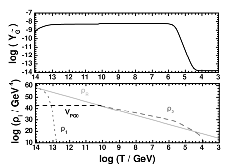
Figure 2: The evolution of the quantities $\log\rho_{i}$ with $i=1$ (gray dotted line), $i=2$ (gray dashed line), $i={\rm R}$ (gray line), $\log V_{\rm PQ0}$ (black dashed line), and $\log Y_{\widetilde{G}}$ (black solid line) as functions of $\log T$ for $\kappa=0.0023,{\mbox{\sl a}}=-0.011,~{}b=-0.01$ and the values of the remaining parameters shown in Eq. (5.4). For the employed vales of parameters, the requirements of Sec. 5.1 are fulfilled.

5 Testing Against Observations

We below exhibit the constraints that we impose on our cosmological set-up in Sec. 5.1 and delineate the allowed parameter space of our model in Sec. 5.2.

5.1 Observational Constraints

The parameters of our model can be restricted imposing the following requirements – note that in the point (v) below we adopt an updated, compared to our analysis in Ref. [1], version of the relevant constraint :

• The violation of the instability conditions in Eq. (23) occurs according to the desired order.

• The number of $e$-foldings $N_{\rm HI*}$ that the scale $k_{*}=0.002/{\rm Mpc}$ suffered during FHI has to be sufficient to resolve the horizon and flatness problems of Standard Big Bang cosmology:

  $$N_{\rm HI*}=N_{\rm HI}-N_{*}\simeq 23+{2\over 3}\ln{V^{1/4}_{\rm HI0}\over{1~{}{\rm GeV}}}-{1\over 3}\ln{V^{1/4}_{\rm PQ0}\over{1~{}{\rm GeV}}}+{1\over 3}\ln{T_{\rm 1rh}T_{\rm 2rh}\over{1~{}{\rm GeV}^{2}}}\>,$$ (38)

  where $N_{*}$ and $N_{\rm HI}$ are the values of $N$ from the onset of FHI until $k_{*}$ crossed outside the horizon of FHI and the end of FHI, respectively. $N_{\rm HI}$ is the largest $N$ at which we obtain violation of Eq. (23a) or of the condition:

  $${\sf max}\{\epsilon(\sigma(N)),|\eta(\sigma(N))|\}\leq 1,~{}~{}\mbox{with}~{}~{}\epsilon\simeq{m^{2}_{\rm P}\over 2}\left(\frac{V_{\rm HI,\sigma}}{V_{\rm HI}}\right)^{2}~{}~{}\mbox{and}~{}~{}\eta\simeq m^{2}_{\rm P}~{}\frac{V_{\rm HI,\sigma\sigma}}{V_{\rm HI}}\>\cdot$$ (39)

• The power spectrum of the curvature perturbation at $k=k_{*}$ is to be confronted with the WMAP7 data:

  $$\Delta_{\cal R*}=\left.V_{\rm HI}^{3/2}\over{2\sqrt{3}\,\pi m^{3}_{\rm P}}|V_{{\rm HI},\sigma}|\right|_{N=N_{*}}\simeq 4.93\cdot 10^{-5}.$$ (40)

• The mass, $gM$, of the lightest gauge boson at the SUSY vacuum – see Table 3 – is to take the value dictated by the unification of the gauge coupling constants within MSSM, i.e.,

  $${gM}\simeq 2\cdot 10^{16}~{}{\mbox{\rm GeV}}\>\Rightarrow\>M\simeq 2.86\cdot 10^{16}~{}{\mbox{\rm GeV}}~{}~{}\mbox{with}~{}~{}g\simeq 0.7,$$ (41)

  being the value of the unified gauge coupling constant - not to be confused with the coefficient ${\rm g}$ appearing in Eq. (17). Note that $G_{\rm LR}$ is considered embedded in the $SO(10)$.

• The spectral index, $n_{\rm s}$, is to be consistent with the fitting of the WMAP7 results by the $\Lambda$CDM model (with negligible running $\alpha_{\rm s}\simeq 0$), i.e.,

  $$n_{\rm s}=1-6\epsilon(N_{*})\ +\ 2\eta(N_{*})=0.968\pm 0.024~{}\Rightarrow~{}0.944\lesssim n_{\rm s}\lesssim 0.992~{}~{}\mbox{at 95\% c.l.}$$ (42)

• In order for the PQPT to take place after a short temporary domination of $V_{\rm PQ0}$, we require:

  $$\left|P_{\rm PQi}\right|>f_{a}/2~{}\Rightarrow~{}s_{\rm PQi}>f_{a}/A_{p}.$$ (43)

• Assuming unstable $\widetilde{G}$, we impose an upper bound on $Y_{2\widetilde{G}}$ in order to avoid problems with the standard Big Bang nucleosynthesis [15]:

  $$Y_{2\widetilde{G}}\lesssim\left\{\begin{matrix}10^{-14}\hfill\cr 10^{-13}\hfill\cr\end{matrix}\right.~{}~{}~{}~{}\mbox{for $\widetilde{G}$\ mass}~{}~{}~{}~{}m_{\widetilde{G}}\simeq\left\{\begin{matrix}0.69~{}{\rm TeV}\hfill\cr 10.6~{}{\rm TeV.}\hfill\cr\end{matrix}\right.$$ (44)

5.2 Numerical Results

As can be seen from the analysis above, our cosmological set-up depends on the following parameters: $\kappa,~{}\kappa_{a},~{}\lambda,~{}f_{a},~{}\lambda_{\mu},~{}n,~{}{\mbox{\sl a}},~{}b,~{}c,~{}d,~{}e,~{}f,~{}\mbox{and g}.$ We fix throughout our computation:

$$\lambda=0.1,~{}f_{a}=10^{12}~{}{\mbox{\rm GeV}},~{}\kappa_{a}=\lambda_{\mu}=0.01,~{}n=5~{}~{}\mbox{and}~{}~{}c=d=e=f={\rm g}=0.1.$$ (45)

The chosen $f_{a}$ and $\lambda_{\mu}$ result to $\mu\simeq 1~{}{\rm TeV}$ via the first term of the RHS of Eq. (15). Also, the selected $\kappa_{a}$ and $\lambda$ play a crucial role in the determination of $T_{\rm 1rh}$ and $T_{\rm 2rh}$ – via Eq. (30) and (33) and facilitate the violation of the conditions in Eq. (23) in the desired order. Their variation, thought, does not cause drastic changes in the inflationary predictions. The same is also valid for the fixed in Eq. (45) parameters of $K$, in Eq. (17) which – contrary to a and $b$ – do not influence the computation of $m^{2}_{+}$ and $m^{2}_{-}$. As we show below, the selected values above give us a wide and natural allowed region of the remaining fundamental inflationary parameters ($\kappa,{\mbox{\sl a}},$ and $b$).

Besides the parameters above, in our computation, we use as input parameters the quantities $N_{*}$ and $f_{\rm HIi}$ with $f=\sigma,~{}s,$ and $q$. We set $f_{\rm HIi}\simeq(1.5-3.5)\cdot 10^{17}~{}{\mbox{\rm GeV}}$ so as to obtain $N_{\rm HI}\simeq 70-140$. We then restrict $M$ and $N_{*}$ so that Eqs. (38) and (40) are fulfilled. It is gratifying that our model supports solutions which simultaneously fulfill Eqs. (40) and (41) contrary to most realizations of FHI – cf. Ref. [6] – which requires, via Eq. (40), $M$’s lower than those indicated in Eq. (41). We finally check if the preferred hierarchy in the violation of Eqs. (23a) and (23b) is achieved and proceed imposing the requirements (v) - (vii) of Sec. 5.1.

Letting a vary for a number of fixed values of $b$, we can depict the values allowed by all the constraints of Sec. 5 in the $\kappa-{\mbox{\sl a}}$ plane – see the left plot of Fig. 3. The various lines terminate at low [high] $\kappa$’s due to the saturation of Eq. (42) from below [above]. We readily conclude that the allowed $({\mbox{\sl a}},b)$’s for fixed $n_{\rm s}$ are almost $\kappa$-independent. This is because $m^{2}_{-}$ is fixed too. In particular, for $n_{\rm s}=0.944,~{}0.968$ and $0.992$, we have $-m^{2}_{-}\simeq 0.0179,~{}0.0125$ and $0.0078$ and $\kappa=0.00125,0.002$ and $0.0037$, respectively. In all cases, $m^{2}_{+}\simeq 1.82$, $Y_{1\widetilde{G}}\simeq 5\cdot 10^{-9}$ and $Y_{2\widetilde{G}}\simeq 2\cdot 10^{-14}$. Therefore, our scenario can be realized for both signs of a and $b$, contrary to the cases studied in Ref. [6] where negative $b$’s are necessitated. Also, compared the extracted $Y_{2\widetilde{G}}$’s with the bounds of Eq. (44), we infer that $\widetilde{G}$ with masses even lower than $10~{}{\rm TeV}$ become observationally safe.

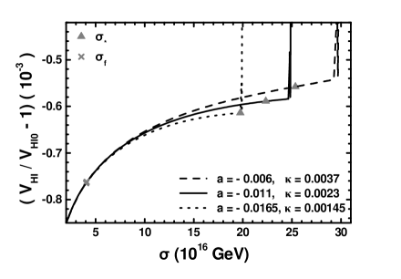
Figure 3: Allowed values by the requirements of Sec. 5.1 in the $\kappa-{\mbox{\sl a}}$ plane for various $b$’s indicated on the curves (left) and the variation of $V_{\rm HI}$ as a function of $\sigma$ for $b=-0.01$ and $({\mbox{\sl a}},\kappa)$’s indicated in the graph (right). In both graphs we use the values of the parameters shown in Eq. (5.4). For the right graph we set $f_{\rm HIi}=3\cdot 10^{17}~{}{\mbox{\rm GeV}}$ ($n_{\rm s}=0.992$, dashed line) or $f_{\rm HIi}=2.5\cdot 10^{17}~{}{\mbox{\rm GeV}}$ ($n_{\rm s}=0.968$, solid line) or $f_{\rm HIi}=2\cdot 10^{17}~{}{\mbox{\rm GeV}}$ ($n_{\rm s}=0.944$, dotted line). The values corresponding to $\sigma_{*}$ and $\sigma_{\rm f}$ are also depicted.

One of the outstanding features of our proposal is that the reduction of $n_{\rm s}$ can be attained without disturbing the monotonicity of the potential – cf. Ref. [6]. This fact is highlighted in the right plot of Fig. 3, where we present the variation of the inflationary potential $V_{\rm HI}$ as a function of $\sigma$, for $b=-0.01$ and three pairs of a and $\kappa$’s, shown in the graph, corresponding to $n_{\rm s}=0.944$ (dotted line), $0.968$ (solid line) and $0.992$ (dashed line). The values corresponding to $\sigma_{*}$ and $\sigma_{\rm f}$ are also designed. We observe that for large $\sigma$’s, $V_{\rm HI}$ develops an oscillatory behavior due to the initial oscillations of $s$ and $q$ – see Fig. 1. However, $V_{\rm HI}$ for lower $\sigma$’s remains monotonic and, therefore, no complications arise in the realization of FHI.

6 Conclusions

We showed that, combining FHI with a PQPT based on renormalizable superpotential terms, we can obtain: (i) Observationally viable FHI at the SUSY GUT scale with natural values, $\pm(0.01-0.1)$, for the model parameters; (ii) a simultaneous resolution of the strong CP and $\mu$ problems of MSSM; (iii) a second stage of reheating after PQPT, which leads to observationally safe values of the $\widetilde{G}$ abundance. An important prerequisite for all these is that the field, which triggers PQPT, remains after FHI well above the PQ scale thanks to (i) its participation in the SUGRA and logarithmic corrections during FHI and (ii) the high reheat temperature after the same period. A noteworthy open issue of our scenario is this of baryogenesis which cannot be processed via non-thermal leptogenesis [4] since the produced lepton asymmetry after FHI is efficiently diluted.

References

- [1] G. Lazarides and C. Pallis, F-term hybrid inflation followed by a Peccei-Quinn phase transition, Phys. Rev. D 82, 063535 (2010) [arXiv:1007.1558].
- [2] E.J. Copeland et al., False vacuum inflation with Einstein gravity, Phys. Rev. D 49, 6410 (1994) [astro-ph/9401011].
- [3] G.R. Dvali, Q. Shafi, and R.K. Schaefer, Large scale structure and supersymmetric inflation without fine tuning, Phys. Rev. Lett. 73, 1886 (1994) [hep-ph/9406319].
- [4] G. Lazarides, R.K. Schaefer, and Q. Shafi, Supersymmetric inflation with constraints on superheavy neutrino masses, Phys. Rev. D 56, 1324 (1997) [hep-ph/9608256].
- [5] E. Komatsu et al. Seven-year Wilkinson Microwave Anisotropy Probe (WMAP) observations: cosmological interpretation, Astrophys. J. Suppl. 192, 18 (2011) [arXiv:1001.4538].
- [6] B. Garbrecht, C. Pallis, and A. Pilaftsis, Anatomy of F(D)-term hybrid inflation, JHEP 12, 038 (2006) [hep-ph/0605264]; M. Bastero-Gil, S.F. King, and Q. Shafi, Hybrid inflation with non-minimal Kahler potential, Phys. Lett. B 651, 345 (2007) [hep-ph/0604198].
- [7] L. Boubekeur and D. Lyth, Hilltop inflation, JCAP 07, 010 (2005) [hep-ph/0502047].
- [8] R.Peccei and H.Quinn,CP conservation in the presence of instantons, Phys. Rev. Lett. 38,1440 (1977).
- [9] J.E. Kim, A common scale for the invisible axion, local SUSY GUTs and saxino decay, Phys. Lett. B 136, 378 (1984); T. Goto and M. Yamaguchi, Is axino dark matter possible in supergravity?, Phys. Lett. B 276, 103 (1992).
- [10] P. Sikivie, Axions, domain walls, and the early Universe, Phys. Rev. D 48, 1156 (1982).
- [11] H. Georgi and M.B. Wise, Hiding the invisible axion, Phys. Lett. B 116, 123 (1982).
- [12] J.E. Kim and H.P. Nilles, The mu problem and the strong CP problem, Phys. Lett. B 138, 150 (1984).
- [13] C. Panagiotakopoulos and N. Tetradis, Two stage inflation as a solution to the initial condition problem of hybrid inflation, Phys. Rev. D 59, 083502 (1999) [hep-ph/9710526].
- [14] M. Bolz, A. Brandenburg, and W. Buchmüller, Thermal production of gravitinos, Nucl. Phys. B606, 518 (2001); ibid. B790, 336 (2008) (E) [hep-ph/0012052].
- [15] M. Kawasaki, K. Kohri and T. Moroi, Hadronic decay of late - decaying particles and Big-Bang nucleosynthesis, Phys. Lett. B 625, 7 (2005) [astro-ph/0402490].
- [16] J. Rocher and M. Sakellariadou, Supersymmetric grand unified theories and cosmology, JCAP 03, 004 (2005) [hep-ph/0406120]; R. Jeannerot and M. Postma, Confronting hybrid inflation in supergravity with CMB data, JHEP 05, 071 (2005) [hep-ph/0503146].
- [17] M.E. Peskin, Supersymmetry in elementary particle physics, arXiv:0801.1928.
- [18] S. Coleman and E. Weinberg, Radiative corrections as the origin of spontaneous symmetry breaking, Phys. Rev. D 7, 1888 (1973).
- [19] K.I. Izawa, M. Kawasaki, and T. Yanagida, Dynamical tuning of the initial condition for new inflation in supergravity, Phys. Lett. B 411, 249 (1997) [hep-ph/9707201]; M. Kawasaki and T. Yanagida, Primordial black hole formation in supergravity, Phys. Rev. D 59,043512 (1999) [hep-ph/9807544].
- [20] D.H. Lyth and T. Moroi, The masses of weakly coupled scalar fields in the early universe, JHEP 05, 004 (2004) [hep-ph/0402174].