Efficient implementations of minimum-cost flow algorithms
Abstract
This paper presents efficient implementations of several algorithms for solving the minimum-cost network flow problem. Various practical heuristics and other important implementation aspects are also discussed. A novel result of this work is the application of Goldberg’s recent partial augment-relabel method in the cost-scaling algorithm. The presented implementations are available as part of the LEMON open source C++ optimization library (http://lemon.cs.elte.hu/). The performance of these codes is compared to well-known and efficient minimum-cost flow solvers, namely CS2, RelaxIV, MCF, and the corresponding method of the LEDA library. According to thorough experimental analysis, the presented cost-scaling and network simplex implementations turned out to be more efficient than LEDA and MCF. Furthermore, the cost-scaling implementation is competitive with CS2. The RelaxIV algorithm is often much slower than the other codes, although it is quite efficient on particular problem instances.
Dept. of Computer Science and
MTA-ELTE Egerváry Research Group
Eötvös Loránd University
Budapest, Hungary
email: kiraly@cs.elte.hu
ChemAxon Ltd. and
Dept. of Algorithms and Applications
Eötvös Loránd University
Budapest, Hungary
email: kpeter@inf.elte.hu
1 Introduction
Network flow theory comprises a wide range of optimization models, which have countless applications in various fields. One of the most fundamental network flow problems is the minimum-cost flow (MCF) problem. It seeks a minimum-cost transportation of a specified amount of a commodity from a set of supply nodes to a set of demand nodes in a directed network with capacity constraints and linear cost functions defined on the arcs. This problem directly arises in various real-world applications in the fields of transportation, logistics, telecommunication, network design, resource planning, scheduling, and many other industries. Moreover, it also arises as a subproblem in more complex optimization tasks, such as multicommodity flow problems. For a comprehensive study of the theory, algorithms, and applications of network flows, see the book of Ahuja, Magnanti, and Orlin [3].
The MCF problem and its solution methods have been the object of intensive research for decades and they have enormous literature. Numerous algorithms have been developed and studied both from theoretical and practical aspects (see the books [26, 13, 48, 3, 64, 52]). Efficient implementation and profound experimental analysis of these algorithms are also of high interest to the operations research community (for example, see [10, 41, 8, 57, 33, 11, 28]). Nowadays, several commercial and non-commercial MCF solvers are available under different license terms.
The primary goal of our research is to provide highly efficient and robust open source implementations of different MCF algorithms and to compare their performance in practice. Preliminary work was published in [49]. This paper presents a more detailed discussion of our implementations along with extensive benchmark testing on a wide range of problem instances.
In order to achieve a comprehensive study, the following algorithms were implemented: SCC: a simple cycle-canceling algorithm; MMCC: minimum-mean cycle-canceling algorithm; CAT: cancel-and-tighten algorithm; SSP: successive shortest path algorithm; CAS: capacity-scaling algorithm; COS: cost-scaling algorithm in three different variants; and NS: primal network simplex method with five different pivot strategies. All of these methods are generally known and well-studied algorithms, our contribution is their efficient implementation with some new heuristics and practical considerations.
According to the authors knowledge, our implementation of the cost-scaling algorithm is the first to apply Goldberg’s recent partial augment-relabel method, which was originally developed to solve the maximum flow problem efficiently [34]. Its utilization in MCF algorithms was also suggested, but was not investigated by Goldberg. According to our tests, this new idea turned out to be a considerable improvement in the cost-scaling MCF algorithm similarly to Goldberg’s results on the maximum flow algorithm.
This paper also presents an empirical evaluation of our implementations and their variants. Numerous benchmark tests were performed on many kinds of large-scale networks containing up to millions of nodes and arcs. These problem instances were created either using well-known random generators, namely NETGEN and GOTO, or based on networks arising in real-life problems. The presented results demonstrate the relative performance of the solution methods and give some guidelines for selecting an MCF algorithm that is suitable for a desired application domain.
Our fastest implementations were also compared to four highly regarded minimum-cost flow solvers: CS2 code of Goldberg and Cherkassky [33, 16], an efficient authoritative implementation of the cost-scaling push-relabel algorithm that has served as a benchmark for a long time; the LEDA library [54], which also implements the cost-scaling algorithm; Löbel’s MCF code [57, 58], which implements the network simplex algorithm; and RelaxIV [27], a C++ translation of the authoritative FORTRAN implementation of the relaxation algorithm due to Bertsekas and Tseng [8, 7]. We henceforth refer to the MCF code as MCFZIB in order to differentiate it from the problem itself. The experiments we conducted show that our cost-scaling implementation is more efficient than LEDA and performs similarly to or slightly slower than CS2. Our network simplex code clearly outperforms MCFZIB and it is the fastest implementation for solving relatively small problem instances (up to a few thousands of nodes). For large networks, however, the cost-scaling codes are usually more efficient than the network simplex algorithms. The performance of RelaxIV turned out to be fluctuating: it is one of the fastest implementations for solving certain kinds of problem instances, but it is very slow for other instances. The detailed experimental results can be found in Section 4.
The implementations presented in this paper are available with full source codes as part of the LEMON optimization library [55]. LEMON is an abbreviation of Library for Efficient Modeling and Optimization in Networks. It is an open source C++ template library with focus on combinatorial optimization tasks related mainly to graphs and networks. It provides easy-to-use and highly efficient implementations of graph algorithms and related data structures, which help solving complex real-life optimization problems. The LEMON project is maintained by the MTA-ELTE Egerváry Research Group on Combinatorial Optimization (EGRES) [25] at the Department of Operations Research, Eötvös Loránd University, Budapest, Hungary. The library is also a member of the COIN-OR initiative [14], a collection of open source projects related to operations research. LEMON applies a very permissive licensing scheme that makes it favorable for commercial and non-commercial software development as well as for research activities. For more information about LEMON, the readers are referred to the introductory paper [21] and to the web site of the library: http://lemon.cs.elte.hu/.
The rest of this paper is organized as follows. Section 2 briefly introduces the MCF problem along with the used notations and theorems. Section 3 describes the implemented algorithms and their variants. Section 4 presents the main experimental results. Finally, the conclusions are drawn in Section 5.
2 The minimum-cost flow problem
2.1 Definitions and notations
The minimum-cost flow (MCF) problem is defined as follows. Let be a weakly connected directed graph consisting of nodes and arcs. We associate with each arc a capacity (upper bound) and a cost , which denotes the cost per unit flow on the arc. Each node has a signed supply value . If , then node is called a supply node with a supply of ; if , then node is called a demand node with a demand of ; and if , then node is referred to as a transshipment node. We assume that all data are integer and we wish to find an integer-valued flow of minimum total cost satisfying the supply-demand constraints at all nodes and the capacity constraints on all arcs. The solution of the problem is represented by flow values assigned to the arcs. Therefore, the MCF problem can be stated as
| (1a) | |||
| subject to | |||
| (1b) | |||
| (1c) | |||
We refer to (1b) as flow conservation constraints and (1c) as capacity constraints. A solution vector is called feasible if it satisfies all constraints defined in (1b) and (1c), and it is called optimal if it also minimizes the total flow cost (1a) over the feasible solutions.
The flow conservation constraints (1b) imply that the sum of the node supply values is required to be zero, that is, , in order to have a feasible solution to the MCF problem:
Without loss of generality, we may further assume that all arc capacities are finite, all arc costs are nonnegative, and the problem has a feasible solution [3].
There are several other problem formulations that are equivalent to the above definition, for instance, the minimum-cost circulation problem, the uncapacitated minimum-cost flow problem, and the transportation problem. However, this definition is quite common in the literature.
Flow algorithms and related theorems usually rely on the concept of residual networks [26, 13, 3, 64, 52]. For a given feasible flow , the corresponding residual network is defined as follows. Let be a directed graph that contains forward and backward arcs on the original node set . A forward arc corresponds to each original arc for which the residual capacity is positive. A backward arc corresponds to each original arc for which the residual capacity is positive. The cost of a forward arc is defined as , while the cost of a backward arc is .
The concept of pseudoflows is also important for several flow algorithms. A pseudoflow is a function defined on the arcs that satisfies only the nonnegativity and capacity constraints (1c) but might violate the flow conservation constraints (1b). A feasible flow is also a pseudoflow. In case of a pseudoflow , a node might have a certain amount of undelivered supply or unfulfilled demand, which is called the excess or deficit of the node, respectively. Formally, the signed excess value of a node with respect to a pseudoflow is defined as
| (2) |
If , node is referred to as an excess node with an excess of ; and if , node is called a deficit node with a deficit of . Note that , that is, the total excess of the nodes equals to the total deficit. The residual network corresponding to a pseudoflow is defined in the same way as in case of a feasible flow.
The running time of an MCF algorithm is measured as a function of the size of the network and the magnitudes of the input data. Let henceforth denote the largest node supply or arc capacity:
| (3) |
and let denote the largest arc cost:
| (4) |
An algorithm is referred to as pseudo-polynomial if its running time is bounded by a polynomial function in the dimensions of the problem and the magnitudes of the numerical data, namely, , , , and . These algorithms technically run in exponential time with respect to the size of the input and they are therefore not considered polynomial. A (weakly) polynomial algorithm is one that runs in time polynomial in the input size, namely, , , , and . Furthermore, an algorithm is called strongly polynomial if its running time depends upon only on the inherent dimensions of the problem, that is, it runs in time polynomial in and regardless of the numerical input data.
2.2 Optimality conditions
In the followings, we formulate optimality conditions for the MCF problem in terms of the residual network as well as the original network. These fundamental theorems are useful in several aspects. Not only do they provide simple methods for verifying the optimality of a certain solution, but they also suggest algorithms for solving the problem. These results are discussed in [26, 13, 3, 64, 52].
Theorem 1 (Negative cycle optimality conditions)
A feasible solution of the MCF problem is optimal if and only if the residual network contains no directed cycle of negative total cost.
This theorem is a consequence of the observation that any feasible flow can be decomposed into a finite set of augmenting paths and cycles.
We also introduce two equivalent formulations of optimality conditions that rely on the notions of node potentials and reduced costs. We associate with each node a signed value , which is referred to as the potential of node . Actually, can be viewed as the linear programming dual variable corresponding to the flow conservation constraint of node (see [3]). With respect to a given potential function , the reduced cost of an arc is defined as
| (5) |
Note that measures the relative cost of the arc with respect to the potentials of its end-nodes.
This concept allows us to formulate the following optimality conditions.
Theorem 2 (Reduced cost optimality conditions)
A feasible solution of the MCF problem is optimal if and only if for some node potential function , the reduced cost of each arc in the residual network is nonnegative:
| (6) |
Note that the total reduced cost of a directed cycle with respect to any potential function equals to the original cost of the cycle. Therefore, the conditions of Theorem 2 obviously imply the negative cycle optimality conditions defined in Theorem 1. Furthermore, a constructive proof exists for the converse result. For an optimal flow , corresponding optimal node potentials can be obtained by solving a shortest path problem in the residual network.
Theorem 2 can be restated in terms of the original network as follows.
Theorem 3 (Complementary slackness optimality conditions)
A feasible solution of the MCF problem is optimal if and only if for some node potential function , the following complementary slackness conditions hold for each arc of the original network:
| (7a) | |||
| (7b) | |||
| (7c) | |||
In addition to these exact optimality conditions, the characterization of approximate optimality is also of particular importance. Several algorithms rely on the concept of -optimality. For a given , a feasible flow or a pseudoflow is called -optimal if for some node potential function , the reduced cost of each arc in the residual network is at least , that is,
| (8) |
These conditions are the relaxations of the reduced cost optimality conditions defined in Theorem 2 and are equivalent to them when . The -optimality conditions can also be restated in terms of the original network to obtain the relaxations of the complementary slackness optimality conditions defined in Theorem 3.
The following lemma formulates two simple observations that are related to -optimality.
Lemma 4
Any feasible solution of the MCF problem is -optimal if . Moreover, if the arc cost are integer and , then an -optimal feasible flow is an optimal solution.
Note that an -optimal flow is also -optimal for all and hence the approximate optimality of is best indicated by the smallest value for which is -optimal. This minimum value is referred to as . The following theorem reveals an inherent connection between and the minimum-mean cycles of the residual network. The mean cost of a directed cycle is defined as its total cost divided by the number of arcs in the cycle.
Theorem 5
For a non-optimal feasible solution of the MCF problem, equals to the negative of the minimum-mean cost of a directed cycle in the residual network . For an optimal solution , .
Therefore, can be computed by finding a directed cycle of minimum-mean cost, which can be carried out in time [46]. Another related problem is to find an appropriate potential function for an -optimal flow or pseudoflow so that they satisfy the -optimality conditions. Similarly to the problem of finding optimal node potentials, this problem can also be solved by performing a shortest path computation in but with a modified cost function for which for each arc in . See, for example, [3, 29] for the proof of all these results related to -optimality.
2.3 Solution methods
The MCF problem and its solution methods have a rich history spanning more than fifty years. Researchers first studied a classical special case of the MCF problem, the so-called transportation problem, in which the network consists only of supply and demand nodes. Dantzig was the first to solve the transportation problem by specializing his famous linear programming method, the simplex algorithm. Later, he also applied this approach to the MCF problem and developed a solution method that is known as the network simplex algorithm. These results are discussed in Dantzig’s book [18].
Ford and Fulkerson developed the first combinatorial algorithms for the uncapacitated and capacitated transportation problems by generalizing Kuhn’s remarkable Hungarian Method [53]. Ford and Fulkerson later proposed a similar primal–dual algorithm for the MCF problem, as well. Their results are presented in the book [26].
In the next few years, other algorithmic approaches were also suggested, namely, the successive shortest path algorithm, the out-of-kilter algorithm, and the cycle-canceling algorithm. These methods, however, do not run in polynomial time. Therefore, both theoretical and practical expectations motivated further research on developing more efficient algorithms. Edmonds and Karp [24] introduced the scaling technique and developed the first weakly polynomial-time algorithm for solving the MCF problem. Later, other researchers also recognized the significant value of this approach and proposed various scaling algorithms. The problem of finding a strongly polynomial-time MCF algorithm, however, remained a challenging open question for several years. Tardos [67] developed the first such algorithm, which was followed by many other methods providing improved running time bounds.
Besides theoretical aspects, efficient implementation and computational evaluation of MCF algorithms have also been an object of intensive research. The network simplex algorithm became quite popular in practice when efficient spanning tree labeling techniques were developed to improve its performance. Later, other algorithms also turned out to be quite efficient. Implementations of relaxation and cost-scaling algorithms were reported to be competitive with the fastest network simplex codes.
Detailed discussion and complexity survey of MCF algorithms can be found in, for example, [3, 64, 52]. Table 1 provides a brief summary of the MCF algorithms having best theoretical running time. Recall from Section 2.1 that and denote the number of nodes and arcs in the network, respectively; denotes the maximum of supply values and arc capacities; and denotes the largest arc cost. Furthermore, let denote the running time of any algorithm solving the single-source shortest path problem in a directed graph with nodes, arcs, and a nonnegative length function. Dijkstra’s algorithm with Fibonacci heaps provides an bound for [64, 15, 52].
| Edmonds and Karp [24]; Tomizawa [70] | |
| successive shortest path | |
| Edmonds and Karp [24] | |
| capacity-scaling | |
| Orlin [60] | |
| enhanced capacity-scaling | |
| Goldberg and Tarjan [38] | |
| generalized cost-scaling | |
| Ahuja, Goldberg, Orlin, and Tarjan [1] | |
| double scaling | |
| Gabow and Tarjan [30] | |
| Gabow and Tarjan [30] |
3 Implemented algorithms
This section discusses the algorithms we implemented as well as the most important heuristics and other practical improvements. All of these methods are well-studied in the literature. Their profound theoretical analysis with the proof of correctness and running time can be found in [3] and in other papers and books cited later in this section. The contribution of this paper is the efficient implementation and empirical analysis of several variants of these algorithms. For further details of our implementations, the readers are referred to the documentation and the source code of the LEMON library [55].
Table 2 provides an overview of the implemented algorithms and their worst-case running time. The same notations are used as in the previous section. Two of these algorithms perform shortest path computations with nonnegative length functions. Our implementations use Dijkstra’s algorithm with binary heaps by default, hence . Note that some of these algorithms have other variants with better theoretical running time, but our research especially focused on the practical performance of them. The given running time bounds correspond to the actual implementations.
| Alg. | Name | Running time |
|---|---|---|
| SCC | simple cycle-canceling | |
| MMCC | minimum-mean cycle-canceling | |
| CAT | cancel-and-tighten | |
| SSP | successive shortest path | |
| CAS | capacity-scaling | |
| COS | cost-scaling | |
| NS | network simplex |
3.1 Cycle-canceling algorithms
Cycle-canceling is one of the simplest methods for solving the MCF problem. This algorithm applies a primal approach based on Theorem 1. A feasible flow is first established, which can be carried out by solving a maximum flow problem. After that, the algorithm throughout maintains feasibility of the solution and gradually decreases its total cost. At each iteration, a directed cycle of negative cost is identified in the residual network and this cycle is canceled by pushing the maximum possible amount of flow along it. When the residual network contains no negative-cost directed cycle, the algorithm terminates and Theorem 1 implies that the solution is optimal.
The cycle-canceling algorithm was proposed by Klein [50]. Its generic version does not specify the order of selecting negative cycles to be canceled, but it runs in pseudo-polynomial time for the MCF problem with integer data. Since the total flow cost is decreased at each iteration and is clearly an upper bound of the flow cost, the algorithm performs iterations if all data are integer. Klein used a label-correcting shortest path algorithm that identifies a negative cycle in time, thus his algorithm runs in time. Later, numerous other variants of the cycle-canceling method were also developed by applying different rules for cycle selection, for example [4, 37, 66]. These algorithms have quite different theoretical and practical behavior. Some of them run in polynomial or even strongly polynomial time.
We implemented three cycle-canceling algorithms, which are discussed in the followings.
Simple cycle-canceling algorithm.
This is a simple version of the cycle-canceling method using the Bellman–Ford algorithm for identifying negative cycles. We henceforth denote this implementation as SCC.
It is well-known that the Bellman–Ford algorithm is capable of detecting a negative-cost directed cycle after performing iterations or detecting that such a cycle does not exist [15]. However, it is not required to perform iterations in most cases. If negative cycles exist in the graph, one or more of them typically appear in the subgraph identified by the predecessor pointers of the nodes after much less iterations. Unfortunately, we do not know the sufficient limit for the number of iterations in advance and searching for cycles using the predecessor pointers at an intermediate step of the algorithm is a relatively slow operation. Therefore, our SCC implementation performs such checking after a successively increasing number of iterations of the Bellman–Ford algorithm. According to our tests, it turned out to be practical to search for negative cycles after executing iterations for each until this limit reaches . It is also beneficial to cancel all node-disjoint negative cycles that can be found at once when Bellman–Ford algorithm is stopped. The worst case time complexity of the SCC algorithm is .
Minimum-mean cycle-canceling algorithm.
This famous special case of the cycle-canceling method was developed by Goldberg and Tarjan [37]. It selects a negative cycle of minimum mean cost to be canceled at each iteration, which yields the simplest MCF algorithm running in strongly polynomial time. We denote this method and our implementation as MMCC.
Recall from Section 2.2 that the mean cost of a directed cycle is defined as its total cost divided by the number of arcs in the cycle. The MMCC algorithm iteratively identifies a directed cycle of minimum-mean cost in the current residual network. If the cost of is negative, then the cycle is canceled and another iteration is performed, otherwise the algorithm terminates with an optimal solution found. It has been proved that this algorithm performs iterations for arbitrary real-valued arc costs and iterations for integer arc costs. The proof of these bounds relies on the concept of -optimality and is rather involved, see [37, 3, 52], although the algorithm is very simple to state.
The MMCC algorithm relies on finding minimum-mean directed cycles in a graph. This optimization problem has also been studied for a long time and several efficient algorithms have been developed for solving it [46, 42, 20, 19, 31]. The best strongly polynomial-time bound for a minimum-mean cycle algorithm is and thus the overall running time of the MMCC algorithm is for the MCF problem with integer data.
We implemented three known algorithms for finding minimum-mean cycles: Karp’s original algorithm [46]; an improved version of this method that is due to Hartmann and Orlin [42]; and Howard’s policy-iteration algorithm [43, 19]. The first two methods run in strongly polynomial time . In contrast, Howard’s algorithm is not known to be polynomial, but it is one of the fastest solution methods in practice [20, 19].
Our experiments also verified that Howard’s algorithm is orders of magnitude faster than the other two methods we implemented. This algorithm gradually approximates the optimal solution by performing linear-time iterations. Relatively few iterations are typically sufficient to find a minimum-mean cycle, but no polynomial upper bound is known. Therefore, we developed a combined method in order to achieve the best performance in practice while keeping the strongly polynomial upper bound on the running time. Howard’s algorithm is run with an explicit limit on the number of iterations. If this limit is reached without finding the optimal solution, we stop Howard’s algorithm and execute the Hartmann–Orlin algorithm. We set this iteration limit to , and hence the overall running time of this combined method is , which equals to the best strongly polynomial bound. In our experiments, the iteration limit was indeed never reached. Thus, the combined method was practically identical to Howard’s algorithm but with a guarantee of worst-case running time .
Cancel-and-tighten algorithm.
This algorithm can be viewed as an improved version of the MMCC algorithm, which is also due to Goldberg and Tarjan [37]. It is faster than MMCC both in theory and practice. This algorithm is henceforth denoted as CAT.
The improvement of the CAT algorithm is based on a more flexible selection of cycles to be canceled. The previously studied cycle-canceling algorithms are pure primal methods in a sense that they do not consider the dual solution at all. In contrast, the CAT algorithm explicitly maintains node potentials, which make the detection of negative residual cycles easier and faster. The key idea of the algorithm is to cancel cycles that consist entirely of negative-cost arcs. Note that the sum of the reduced arc costs along a cycle with respect to any potential function is exactly the same as the original cost of the cycle. Therefore, the algorithm can consider the reduced costs with respect to the current node potentials instead of the original costs. A residual arc is called admissible if its reduced cost is negative; the subgraph of the residual network consisting only of the admissible arcs is called the admissible network; and a directed cycle in the admissible network is referred to as an admissible cycle.
The CAT algorithm performs two main steps at every iteration until the current solution becomes optimal. In the cancel step, admissible cycles are successively canceled until such a cycle does not exist. In the tighten step, the node potentials are modified in order to make more arcs admissible. Despite the MMCC algorithm, this method explicitly utilizes the concept of -optimality. Recall the corresponding definitions and theorems from Section 2.2. The CAT algorithm ensures -optimality of the solution for successively smaller values of . In the tighten step, the potentials are modified so as to satisfy the -optimality conditions for a smaller that is at most times its former value.
The cancel step is the dominant part of the computation. We implemented a straightforward method for this step based on a depth-first traversal of the admissible network. This implementation runs in time as canceling a cycle takes time and at most admissible cycles can be successively canceled without modifying the potential function. Goldberg and Tarjan [37] also showed that using dynamic tree data structures [65], the running time of this step can be reduced to (amortized time per cycle cancellation). However, we did not invest effort in implementing this variant because the cycle-canceling algorithms turned out to be relatively slow in our experimental tests (see Section 4).
The tighten step can be performed in time based on a topological ordering of the nodes with respect to the admissible network. This implementation, however, does not ensure that the overall running time of the algorithm is strongly polynomial. To overcome this drawback, Goldberg and Tarjan [37] suggested to carry out the tighten step in a stricter way after every iterations of the algorithm. In these cases, a minimum-mean cycle computation is performed to exactly determine the smallest value for which the current flow is -optimal (see Theorem 5). Node potentials are also recomputed to correspond to this value. Note that the amortized running time of the tighten step is not affected by this modification. Our implementation, however, performs this stricter tighten step more often, namely after every iterations, because it turned out to be more efficient in practice. This means that the amortized running time of the tighten step becomes , but it is still less than the time of our implementation of the cancel step. The minimum-mean cycle computations are carried out using the same combined algorithm that was applied in the MMCC algorithm.
This algorithm is strongly polynomial. It runs in time for the MCF problem with arbitrary arc costs and in time for integer arc costs, see [37].
The experimental results for these algorithms are presented in Section 4. It turned out that their relative performance depends upon the problem instance, but the CAT algorithm is usually much more efficient than both SCC and MMCC. However, all three of these cycle-canceling algorithms turned out to be slower than the cost-scaling and network simplex methods.
3.2 Augmenting path algorithms
Another fundamental approach for solving the MCF problem is the so-called successive shortest path method. It is a dual ascent algorithm that successively augments flow along shortest paths of the residual network to send the required amount of flow from the supply nodes to the demand nodes. In this sense, this method can be viewed as a generalization of the well-known augmenting path algorithms solving the maximum flow problem, namely the Ford–Fulkerson and Edmonds–Karp algorithms [26, 24, 3, 15].
The successive shortest path algorithm in its inital form was developed independently by Jewell [45], Iri [44], and Busacker and Gowen [12]. They showed that the MCF problem can be solved by a sequence of shortest path computations. Later, Edmonds and Karp [24] and Tomizawa [70] independently suggested the utilization of node potentials in the algorithm to maintain nonnegative arc costs for the shortest path problems. This technique greatly improves both the theoretical and the practical performance of the algorithm. Edmonds and Karp [24] also developed a capacity-scaling variant of this method that runs in polynomial time.
We implemented the standard successive shortest path algorithm applying node potentials as well as the capacity-scaling method. These algorithms and the most important aspects of their implementations are discussed below.
Successive shortest path algorithm.
This algorithm is henceforth denoted as SSP. In contrast to the cycle-canceling method, which maintains a feasible flow and attempts to achieve optimality, the SSP algorithm maintains an optimal pseudoflow and node potentials and attempts to achieve feasibility. Recall from Section 2.1 that a pseudoflow satisfies the nonnegativity and capacity constraints but might violate the flow conservation constraints at some nodes. Such a node has a certain amount of excess or deficit.
The SSP algorithm begins with constant zero pseudoflow and a constant potential function and proceeds by gradually converting into a feasible solution while throughout maintaining the reduced cost optimality conditions defined in Theorem 2. At every iteration, the algorithm selects a node with positive excess and sends flow from this node to an arbitrary deficit node along a shortest path of the residual network with respect to the reduced arc costs. After that, the node potentials are modified using the computed shortest path distances to preserve the reduced cost optimality conditions. These conditions not only verify the optimality of both the primal and the dual solutions, but they also ensure nonnegative arc costs for the consecutive shortest path computations. By sending flow from excess nodes to deficit nodes, the algorithm iteratively decreases the total excess of the nodes until the solution becomes feasible. At the beginning of the algorithm, the total excess is at most and each iteration decreases this value by at least one (in case of integer data), thus the SSP algorithm terminates after path augmentations. The flow conservation constraints are then satisfied at all nodes and hence the solution is both feasible and optimal.
We implemented the SSP algorithm as follows. At each iteration, flow is augmented from the current excess node to a deficit node whose shortest path distance from is minimal. The shortest path searches are carried out using Dijkstra’s algorithm with a heap data structure. We experimented with several heap variants provided by the LEMON library [56] and the standard binary heap structure turned out to be one of the fastest and most robust implementations. Therefore, our SSP implementation uses this data structure by default. This means that a single iteration is performed in time and the overall complexity of the algorithm is . However, one can easily switch to other data structures (for instance, Fibonacci heaps).
The practical performance of the SSP algorithm mainly depends on the shortest path computations. We applied a significant improvement related to these searches, which is discussed, for example, in [3]. At each iteration, it is not necessary to compute the shortest paths to all nodes from the current excess node , but the Dijkstra algorithm can be terminated once it permanently labels a deficit node . The node potentials can also be updated in an alternative way that does not require any modification for those nodes that were not permanently labeled during the shortest path computation. This improvement can be implemented quite easily, but it greatly improves the efficiency of the SSP algorithm in practice.
The representation of the residual network is another important aspect of the implementation. It is possible to implement the SSP algorithm using the original representation of the input network, but in this case, all outgoing and incoming arcs of the current node have to be checked at each step of the shortest path computations. Another possibility is to explicitly maintain the residual network containing only those arcs that have positive residual capacity. However, this implementation would require the updating of the graph structure after each path augmentations, which is time-consuming.
We applied an intermediate solution that turned out to be the most efficient. We store an auxiliary graph that contains all possible forward and backward arcs and also maintain their residual capacities explicitly. All shortest path computations run on by skipping those arcs whose current residual capacity is zero. The flow augmentations are carried out by decreasing the residual capacities of the arcs on the path and increasing the residual capacities of the corresponding reverse arcs. Therefore, we also store for each arc an index to its reverse arc (often referred to as sister arc). The major benefit of this implementation is that this auxiliary graph allows a quite efficient representation. Note that using , only the outgoing arcs of a node have to be traversed during the shortest path searches and is not modified throughout the algorithm. We can, therefore, represent the outgoing arcs of a node in by consecutive integers, which makes it possible to traverse these arcs quite efficiently without iterating over the elements of an array or a linked list.
The reduced arc costs are also required in the shortest path computations. Since these values are frequently modified by adjusting node potentials, it is better to store only the potentials and recompute reduced costs whenever they are needed. Furthermore, we also maintain a signed excess value for each node.
Capacity-scaling algorithm.
This algorithm, which we denote as CAS, is an improved version of the SSP method. It uses a capacity-scaling scheme that reduces the number of iterations from to . This algorithm was devised by Edmonds and Karp [24] as the first weakly polynomial-time solution method for the MCF problem. Our implementation is based on a slightly modified variant that is due to Orlin [60] and also discussed in [3].
The SSP algorithm has a substantial drawback that the shortest path augmentations might deliver relatively small amounts of flow, which results in a large number of iterations. This is overcome in the CAS algorithm by ensuring that each path augmentation carries a sufficiently large amount of flow and hence the number of augmentations is often reduced. The CAS algorithm performs scaling phases for successively smaller values of a parameter . In a -scaling phase, each path augmentation delivers exactly units of flow from a node with at least units of excess to a node with at least units of deficit. The shortest path searches are carried out in the so-called -residual network, which contains only those arcs whose residual capacities are at least . When no such augmenting path is found, the value of is halved and the algorithm proceeds with the next phase. Initially, is set to and the algorithm terminates at the end of the phase in which .
The CAS algorithm maintains the reduced cost optimality conditions only in the -residual network. Each -scaling phase begins with saturating those newly introduced arcs of the current -residual network that do not satisfy the optimality conditions with respect to the current node potentials. The saturations might increase the excess or deficit of some nodes, but these requirements are satisfied in the subsequent phases. At the end of the last phase, which corresponds to , the solution becomes both feasible and optimal since the -residual network then coincides with the residual network.
In order to ensure the weakly polynomial running time of the CAS algorithm, we need an additional assumption that a directed path of sufficiently large capacity exists between each pair of nodes. This condition, however, can easily be achieved by a simple extension of the underlying network as follows. Let denote a designated node of the network (or a newly introduced artificial node). For each other node , we can add new arcs and to the graph with sufficiently large capacities and costs. Under this additional assumption, the CAS algorithm is proved to solve the MCF problem in time [3].
We made some modifications to this version of the CAS algorithm in our implementation. First, it is possible to avoid the above extension of the input graph by allowing that more units of excess or deficit remain at the end of a -scaling phase. In this case, the polynomial running time bound is not proved, but our experiments show that this version does not perform more path augmentations and runs significantly faster in practice. Therefore, our implementation does not extend the input graph by default. Another modification utilizes that the path augmentations of each -scaling phase might be capable of delivering more than units of flow. We send the maximum possible amount of flow along each path similarly to the SSP algorithm. Furthermore, the scaling of the parameter can be carried out using a factor other than two. Let denote an integer scaling factor. is initially set to and divided by at the end of each phase. This means that more path augmentations might be required for the same excess or deficit node in a -scaling phase, but the number of phases is reduced. In our experiments, a factor of turned out to provide the best overall performance, thus this option is used by default.
The CAS algorithm has much in common with the SSP method, thus the practical improvements of the SSP implementation also applies to this algorithm. Our CAS code uses the same representations for the residual network and the associated data. In a -scaling phase, the -residual network is not constructed explicitly, but the arcs with residual capacity less than are skipped during the path searches. Moreover, our CAS implementation also terminates the shortest path computations once an appropriate deficit node is permanently labeled and updates the node potentials accordingly. This idea and the practical data representations substantially improve the performance of the CAS algorithm similarly to the SSP method.
The computational results presented in Section 4 show that the augmenting path algorithms, SSP and CAS, are not robust as their performance greatly depends upon the characteristics of the input. On general problem instances, these algorithms are typically slower than the cost-scaling and network simplex methods, but in certain cases, they turned out to be quite efficient. For example, if the total excess is relatively small and hence a few path augmentations are sufficient to solve the problem, the SSP algorithm is usually the fastest method.
3.3 Cost-scaling algorithm
The cost-scaling technique for the MCF problem was proposed independently by Röck [63] and Bland and Jensen [9]. Goldberg and Tarjan [38] developed an improved method based on these algorithms by also utilizing the concept of -optimality, which is due to Bertsekas [6] and, independently, Tardos [67]. The cost-scaling algorithm of Goldberg and Tarjan, which we henceforth refer to as COS, can be viewed as a generalization of their well-known push-relabel algorithm for the maximum flow problem [36]. The COS algorithm is one of the most efficient solution methods for the MCF problem, both in theory and practice.
The COS algorithm is a primal–dual method that applies a successive approximation scheme by scaling upon the costs. It iteratively produces -optimal primal–dual solution pairs for successively smaller values of . (Recall the definitions and results related to -optimality from Section 2.2.) Initially, and each phase preforms a refine procedure to transform an -optimal solution into an -optimal solution until . At this stage, the algorithm terminates and Lemma 4 implies that an optimal flow is found.
The refine procedure takes an -optimal primal–dual solution pair as input and improves the approximation as follows. First, it saturates each residual arc whose current reduced cost is negative and thereby produces a pseudoflow that is 0-optimal. This means that is also -optimal for any choice of , but it is not necessarily feasible. After this step, the current approximation parameter is halved and the pseudoflow is gradually transformed into a feasible solution again, but in a way that preserves -optimality for the new value of . This is achieved by performing a sequence of push and relabel operations similarly to the push-relabel algorithm for the maximum flow problem.
Let denote the residual capacity of an arc in the residual network corresponding to the current pseudoflow and let denote the signed excess value of node . We call a node active if its current excess is positive. Furthermore, a residual arc is called admissible if its current reduced cost is negative and the subgraph of the residual network consisting only of the admissible arcs is called the admissible network. The refine procedure throughout maintains -optimality and hence holds for each admissible arc . A basic operation selects an active node (i.e., ) and either pushes flow on an admissible residual arc or if no such arc exists, updates the potential of node , which is called relabeling.
A push operation on an admissible residual arc is carried out by sending units of flow from node to node and thereby decreasing and increasing by . This operation introduces the reverse arc into the residual network unless it already had positive residual capacity, but this arc is not admissible since . If an active node has no admissible outgoing arc, a relabel operation decreases its potential by . This means that the reduced cost of each outgoing residual arc of node is also decreased and the reduced cost of each incoming residual arc is increased by . Note that this modification preserves the -optimality conditions while creating new admissible outgoing arcs at node and thus allowing subsequent push operations to carry the excess of node . Consequently, the only operation that can introduce a new admissible arc is the relabeling of node . The refine procedure terminates when no active node remains in the network and hence an -optimal feasible solution is obtained.
It is proved that this generic version of the refine procedure performs relabel operations and push operations and hence runs in time [38, 3]. Furthermore, the number of -scaling phases is , as is initially set to and it is halved at each phase until it decreases below . Consequently, the generic COS algorithm runs in weakly polynomial time . Note, however, that the order in which the basic operations are performed is not specified. Goldberg and Tarjan [38] showed that applying particular selection rules and using complex data structures yield better theoretical running time. They also developed a generalized framework to obtain a strongly polynomial bound on the number of -scaling phases by utilizing the same idea that is exploited in the MMCC and CAT algorithms (see Section 3.1). The best variant they devised runs in time using dynamic trees [38, 65]. Moreover, the COS algorithm turned out to be quite efficient in practice and several complicated heuristics were also developed to improve its performance [33].
We implemented three variants of the COS method that perform the refine procedure rather differently.
Push-relabel variant.
This variant of the COS algorithm is based on the generic version discussed above and hence performs local push and relabel operations in the -scaling phases. We also applied several improvements and efficient heuristics in this implementation according to the ideas found in [38, 3, 35, 33, 11]. In fact, most of these improvements and heuristics are analogous to similar techniques devised for the push-relabel maximum flow algorithm.
The bottleneck of the COS algorithm corresponds to the searching of admissible arcs for the basic operations. Therefore, we applied the same graph representation that is used in the augmenting path algorithms (see Section 3.2) as it is intended to minimize the time required for iterating over the outgoing residual arcs of a node.
Similarly to the capacity-scaling algorithm, the COS method also allows us to use an arbitrary scaling factor . We found that the optimal value depends on the problem, but it was usually between 8 and 24 and the differences were moderate. The default scaling factor is in our implementation, which typically performed very well. Another practical modification targets the issue that the generic COS algorithm performs internal computations with non-integer values of and non-integer node potentials. This drawback can be overcome by multiplying all arc costs by for a given integer scaling factor and by scaling accordingly. Initially, is set to and is divided by in each phase until .
We applied some improvements in the implementation of the refine procedure, as well. For performing the basic operations, we need to check the outgoing residual arcs of each active node for admissibility. These examinations can be made more efficiently if we record a current arc for each active node and continue the search for an admissible outgoing arc from this current arc every time. If an admissible arc is found, we perform a push operation and when we reach the last outgoing arc of an active node without finding an admissible arc, the node is relabeled and its current arc is set to the first outgoing residual arc again. (Recall that the definition of the basic operations imply that only the relabeling of node can introduce a new admissible arc outgoing from node .) Furthermore, the relabel operations are performed in a stricter way. Instead of simply decreasing the potential of a relabeled node by , we decrease the potential by the largest possible amount that does not violate the -optimality conditions. A single relabel operation thereby usually introduce more admissible arcs. This modification significantly improves the overall performance of the algorithm (up to a factor of two).
The strategy for selecting an active node for the next basic operation is also important. The number of active nodes is typically small, thus it is beneficial to keep track of them explicitly. A particular variant of the COS algorithm, known as the wave implementation, selects the active nodes according to a topological ordering with respect to the admissible network. This choice is proved to yield an -time implementation of the refine procedure (instead of ). However, our experiments showed that a simple FIFO selection rule using a queue data structure usually results in less basic operations and better performance in practice, which is in accordance with [11] and [33].
In addition to the implementation aspects discussed so far, some effective heuristics can improve the practical performance of the COS algorithm to a higher extent. We implemented three such improvements out of the four proposed by Goldberg [33]. These heuristics are also discussed in [35] along with detailed experimental evaluation. Their practical effect depends on the problem instances as well as the actual implementation and the parameter settings (for example, the scaling factor ).
The potential refinement (or price refinement) heuristic is based on the observation that an -scaling phase may produce a solution that is not only -optimal, but also -optimal or even optimal. Therefore, an additional step is introduced at the beginning of each phase to check if the current solution is already -optimal. This heuristic attempts to adjust the potentials to satisfy the -optimality conditions, but without modifying the flow. If -optimality is verified, the refine procedure is skipped and another phase is performed. We implemented this potential refinement heuristic using an -time scaling shortest path algorithm [32] as suggested in [33]. Our experiments also verified that this improvement usually eliminates the need for the refine procedure in a few phases, especially the last ones. Furthermore, the potential updates performed in this heuristic step typically reduce the number of basic operations even in case the refine procedure can not be skipped. Consequently, this additional step significantly improves the overall performance of the algorithm in most cases.
Another possible implementation of this heuristic performs a minimum-mean cycle computation in each phase to determine the smallest for which the current flow is -optimal and computes corresponding node potentials. This computation may allow us to skip more than one phase at once, but it is usually slower, even using Howard’s efficient algorithm. Furthermore, this variant can be used to ensure a strongly polynomial bound on the number of phases and thus on the overall running time, as well. However, our experiments showed that the former variant of the potential refinement heuristic, which we use in our final implementation, is clearly superior to this one. This result contradicts the conclusions of [11].
The global update heuristic performs relabel operations on several nodes in one step. It iteratively applies the following set-relabel operation. Let denote a set of nodes such that it contains all deficit nodes, but at least one active node is in . If no admissible arc enters , then the potential of every node in can be increased by without violating the -optimality conditions. Furthermore, it is also shown in [33] that the theoretical running time of the COS algorithm remains unchanged if the global update heuristic is applied only after every relabel operations. In practice, this modification turned out to impose a huge improvement in the efficiency of the algorithm on some problem classes, although it does not help to much or even slightly worsens the performance on other instances. Our implementation of this heuristic follows the instructions presented in [11].
The push-look-ahead heuristic is another practical improvement for the COS algorithm. Its goal is to avoid pushing flow from node to node when a subsequent push operation is likely to send this amount of flow back to node . To achieve this, the maximum allowed amount of flow to be pushed into a node is limited by the sum of its deficit and the residual capacities of its admissible outgoing arcs. However, this idea requires the extension of the relabel operation to those nodes at which this limitation is applied regardless of their current excess values. This heuristic is rather effective in practice, it usually decreases the number of push operations significantly and hence the relabel operations dominate the running time of the COS algorithm. For more details about this heuristic, see [35, 33, 11].
Goldberg [33] also suggests an additional improvement, the arc fixing heuristic. The best version of this method speculatively fixes the flow values for the arcs on which it is not likely to be changed later in the algorithm. These arcs are excluded from the subsequent arc examinations, but in certain cases, they have to be unfixed again. We did not implement this heuristic yet, because it seems to be rather involved and sensitive to parameter settings. However, it would most likely improve the performance of our implementation.
We also remark that dynamic trees [65] can be used in the COS algorithm to perform a number of push operations at once, which improves the theoretical running time [38]. However, they are not likely to be practical due to the computational overhead that these data structures usually impose and because applying the above heuristics, the relabel operations become the bottleneck of the algorithm instead of pushes (see [35, 33]). Therefore, we did not implement this variant.
Augment-relabel variant.
This variant of the COS algorithm performs path augmentations instead of local push operations, but relabeling is heavily used to find augmenting paths. At each step of the refine procedure, this method selects an active node and performs a depth-first search in the admissible network to find an augmenting path to a deficit node. At an intermediate stage, the algorithm maintains an admissible path from an active node to the current node and attempts to extend this path. If node has an admissible outgoing arc , then the path is extended with this arc and node becomes the current node. Otherwise, node is relabeled and if , we step back to the previous node by removing the last arc of the current path. When this search process reaches a deficit node, an augmenting path is found.
The flow augmentation on these admissible paths can be performed in two different ways. The first way is to push the same amount of flow on each arc of an augmenting path, which is bounded by the smallest residual capacity on the path as well as the excess of the starting node . The other apparent implementation pushes the maximum possible amount of flow on every arc of the path. That is, for each arc of the path, units of flow is pushed on the arc, is decreased by , and is increased by . According to our experiments, this variant is slightly superior to the former one, thus it is applied in our implementation.
Note that these path search and flow augmentation methods correspond to a particular sequence of local push and relabel operations. However, the actual push operations are carried out in a delayed and more guided manner, in aware of an admissible path to a deficit node. This helps to avoid such problems for which the push-look-ahead heuristic is devised (see above), but a lot of work may be required to find augmenting paths, especially if they are long.
Since this algorithm can be viewed as a special version of the generic COS method, the same theoretical running time bound applies to it as well as most of the practical improvements. We used the same data representation, improvements and heuristics as for the push-relabel algorithm except for the push-look-ahead heuristic, which is obviously incompatible with this variant. These modifications provided similar performance gains to those measured for the push-relabel variant.
Partial augment-relabel variant.
The third variant of the COS algorithm can be viewed as an intermediate approach between the other two variants. It is based on the partial augment-relabel technique recently proposed by Goldberg [34] as an improvement for the push-relabel maximum flow algorithm. This method turned out to be more efficient and more robust than the classical push-relabel algorithm and Goldberg also suggested the utilization of the same idea in the MCF context. According to the authors knowledge, our implementation of the COS algorithm is the first to incorporate this technique.
The partial augment-relabel algorithm is quite similar to the augment-relabel variant, but it limits the length of the augmenting paths. The path search process is stopped either if a deficit node is reached or if the length of the path reaches a given parameter . In fact, the push-relabel and augment-relabel variants are special cases of this approach for and , respectively. Goldberg [34] suggests small values for the parameter in the maximum flow context, which turned out to apply to the COS algorithm, as well. In our experiments, the optimal value of this parameter was typically between 3 and 8 and the differences were not substantial for such small values of . Our default implementation uses , just like Goldberg’s maximum flow implementation, as it turned out to be quite robust.
Apart from the length limitation for the augmenting paths, this variant is exactly the same as the augment-relabel method. (Actually, they have a common implementation but with different values of the parameter .) However, the partial augment-relabel technique attains a good compromise between the former two approaches and turned out to be clearly superior to them, thus it is our default implementation of the COS algorithm. Unless stated otherwise, we refer to this implementation as COS in the followings.
Section 4 provides experimental results for the COS algorithm and its variants compared to other methods. The classical push-relabel algorithm and especially the partial augment-relabel variant using such heuristics and improvements are highly efficient and robust in practice. In contrast, the augment-relabel variant is often significantly slower.
3.4 Network simplex algorithm
The primal network simplex algorithm, which we henceforth refer to as NS, is one of the most popular solution methods for the MCF problem in practice. It is a specialized version of the well-known linear programming (LP) simplex method that exploits the network structure of the MCF problem and performs the basic operations directly on the graph representation. The LP variables correspond to the arcs of the graph and the LP bases are represented by spanning trees.
The NS algorithm is devised by Dantzig, the inventor of the LP simplex method. He first solved the uncapacitated transportation problem using this approach and later generalized the bounded variable simplex method to directly solve the MCF problem [18]. Although the generic version of the NS algorithm does not run in polynomial time, it turned out to be rather efficient in practice. Therefore, subsequent research focused on efficient implementation of the NS algorithm [10, 5, 48, 41, 57] as well as on developing special variants of both the primal and the dual network simplex methods that run in polynomial time [68, 39, 62, 61, 69]. Detailed discussion of the NS method considering both theoretical and practical aspects can be found in [3] and [47].
The fundamental concept on which the NS algorithm is based is the notion of spanning tree solutions. Such a solution is represented by a partitioning of the node set into three subsets such that each arc in has flow fixed at zero (lower bound), each arc in has flow fixed at the capacity of the arc (upper bound), and the arcs in form an (undirected) spanning tree of the network. The flow on these tree arcs also satisfy the nonnegativity and capacity constraints, but they are not restricted to any of the bounds. It can easily be seen that the flow values on the tree arcs are uniquely determined by the partitioning since there is no cycle in . Furthermore, it is proved that if an instance of the MCF problem has an optimal solution, then it also has an optimal spanning tree solution, which can be found by successively transforming a spanning tree solution to another (see [3]). Actually, these spanning tree solutions correspond to the LP basic feasible solutions of the problem. This observation allows us to implement the simplex method by performing all operations directly on the network, without maintaining the simplex tableau, which makes this approach very efficient.
The standard simplex method maintains a basic feasible solution and gradually improves its objective function value by small transformations, known as pivots. Accordingly, the NS algorithm throughout maintains a spanning tree solution of the MCF problem and successively decreases the total cost of the flow until it becomes optimal. Furthermore, node potentials are also maintained such that the reduced cost of each arc in the spanning tree equals to zero. At each step, a non-tree arc violating its complementary slackness optimality condition (see Theorem 3) is added to the current spanning tree, which uniquely determines a negative cost residual cycle. This cycle is then canceled by augmenting the maximum possible amount of flow on it and a tree arc corresponding to a saturated residual arc is selected to be removed from the tree. The node potentials are also adjusted to preserve the property that the reduced costs of each tree arc is zero and finally, the tree structure is updated. This whole operation transforming a spanning tree solution to another is called pivot. If no suitable entering arc can be found, the current flow is optimal and the algorithm terminates.
In fact, the NS algorithm can also be viewed as a particular variant of the cycle-canceling method (see Section 3.1). Due to the sophisticated method of maintaining spanning tree solutions, however, a negative cycle can be found and canceled much faster (in linear time). On the other hand, an additional technical issue, known as degeneracy, may arise in the NS algorithm. If the spanning tree contains an arc whose flow value equals to zero or the capacity of the arc, then a pivot step may detect a cycle of zero residual capacity. Such degenerate pivots only modify the spanning tree, but the flow itself remains unchanged. Consequently, it is possible that several consecutive pivots do not actually decrease the flow cost (known as stalling) or, which is even worse, the same spanning tree solution occurs multiple times and hence the algorithm does not necessarily terminate in a finite number of iterations (known as cycling). Experiments with certain classes of large-scale MCF problems showed that more than 90% of the pivots may be degenerate.
A simple and popular technique to overcome such difficulties is based on the concept of strongly feasible spanning tree solutions. A spanning tree solution is called strongly feasible if a positive amount of flow can be sent from each node to a designated root node of the spanning tree along the tree path without violating the nonnegativity and capacity constraints. Using an appropriate rule for selecting the leaving arcs, the NS algorithm can throughout maintain a strongly feasible spanning tree. This technique is proved to ensure that the algorithm terminates in a finite number of iterations [3]. Furthermore, it substantially decreases the number of degenerate pivots in practice and hence makes the algorithm faster.
It can be shown, using a perturbation technique, that the NS algorithm maintaining a strongly feasible spanning tree solution performs pivots for the MCF problem with integer data regardless of the selection rule of entering arcs [2]. An entering arc can be found in time and using an appropriate labeling technique, the spanning tree structure can be updated in time. Therefore, a single pivot takes time and the total running time of the NS algorithm is . However, this bound does not reflect to the typical performance of the algorithm in practice.
The implementation of the primal NS algorithm is based on a practical storage scheme of the spanning tree solutions that makes it possible to perform the basic operations of the algorithm efficiently. The book of Kennington and Helgason [48] discusses several such spanning tree data structures along with methods for updating them during the iterations of the algorithm. A quite popular approach, sometimes referred to as the ATI (Augmented Threaded Index) method, represents a spanning tree as follows. The tree has a designated root node and three indices is stored for each node in the tree: the depth of the node (i.e., the distance from the root node in the tree), the parent of the node in the tree, and a thread index which is used to define a depth-first traversal of the spanning tree. This storage scheme and its update mechanism are discussed in detail in [47] and [3]. The ATI technique has an improved version, which is due to Barr, Glover, and Klingman [5] and is usually referred to as the XTI (eXtended Threaded Index) method. The XTI scheme replaces the depth index by two indices for each node: the number of successors of the node in the tree and the last successor of the node according to the traversal defined by the thread index. Other approaches, for example the so-called API and XPI methods, are also often applied.
We implemented the primal NS algorithm using both ATI and XTI techniques. The latter one has two advantages over the ATI method. First, the XTI indices can be updated more efficiently since a tree alteration of a single pivot usually modifies the depth of several nodes in subtrees that are moved from a position to another, while the set of successors is typically modified only for a much smaller number of nodes. In addition, the XTI method also allow an improved updating process for the node potentials. Note that by removing the leaving arc, the current spanning tree is divided into two subtrees, which are then connected again by the entering arc. In order to preserve zero reduced costs for the tree arcs, we have to increase the potential of each node in one of the subtrees by a certain constant value or decrease the potential of each node in the other subtree by . The XTI scheme makes it possible to immediately determine which subtree is smaller and to perform the update process on the smaller subtree.
Although the XTI labeling method is not as widely known and popular as the simpler ATI method, our experiments showed that it is much more efficient than ATI on all problem instances. Therefore, the final version of our code only implements the XTI technique. The substantial performance gain of this approach is due to the first advantage mentioned above. In contrast, we found that the alternative potential update is not so important, because the subtree containing the root node turned out to be the bigger one in virtually all pivots. Moreover, we can easily avoid overflow problems related to node potentials and reduced costs if the potential of the root node is not modified throughout the algorithm. Therefore, we decided to update potentials in the subtree not containing the root node in every step. We also applied an important improvement in the implementation of the XTI method. An additional reverse thread index is also stored for each node and hence the depth-first traversal is represented by a doubly-linked list. This modification turned out to substantially improve the performance of the update process. In fact, the inventors of the XTI technique also discussed this improvement [5], but they did not applied it to reduce the memory requirements of the representation. (However, note that enormous progress has been made on the computers since the time when that paper was written.)
Another interesting aspect of the data representation for the NS algorithm is that we need not traverse the incident arcs of nodes throughout the algorithm, although such examinations are crucial in other algorithms. Therefore, we applied a quite simple and unusual graph representation to implement the NS algorithm. The nodes and arcs are represented by consecutive integers and we store the source and target nodes for each arc (in arrays), but we do not keep track of the incident arcs of a node at all.
The NS algorithm also requires an initial spanning tree solution to start with. It is possible to transform any feasible solution to a spanning tree solution such that the total cost of is less than or equal to the total cost of . Furthermore, the required spanning tree indices can also be computed by a depth-first traversal of the tree arcs. However, artificial initialization techniques are much more common in practice. An artificial root node with zero supply is typically added to the network as well as artificial arcs with sufficiently large capacities and costs. Recall that the signed supply value of node is denoted as . For each original node , we add a new arc to the network if and add a new arc otherwise. We can set the capacity of each new arc to and its cost to . In this extended network, we can easily construct a strongly feasible spanning tree solution as follows. For each original arc , let and for each original node , let if and let otherwise. The initialization of the tree indices and the node potentials is straightforward in this case. Furthermore, note that an optimal solution in the extended network does not send flow on artificial arcs due to their large costs unless the original problem is infeasible.
We experimented with both ways of initialization and it turned out that the artificial method usually provides better overall performance mainly because of two reasons. First, the artificial spanning tree solution can be constructed easily and quickly. Second, it allows efficient tree update for the first few pivots as the depth of the tree is rather small. Therefore, we decided to use only this variant in our final implementation. The strongly feasibility is preserved throughout the algorithm by carefully selecting the leaving arc whenever multiple residual arcs are saturated by a pivot step (see [47, 3] for details).
One of the most crucial aspects of the NS algorithm, which is not considered so far, is the selection the entering arcs. Recall that the reduced cost of each tree arc is zero and each non-tree arc has a flow value fixed either at zero or the capacity of the arc. Therefore, a non-tree arc allows flow augmentation only in one direction. If the reduced cost of the residual arc associated with this direction is negative, the arc can be selected to enter the tree. In this case, a negative-cost residual cycle is formed by this arc and the unique tree path connecting nodes and (these tree arcs have zero reduced costs). To implement the NS algorithm, we require a method for selecting such an entering arc at each iteration, which is usually referred to as pivot rule or pricing strategy. The applied method affects the “goodness” of the entering arcs and thereby the number of iterations as well as the average time required for selecting an entering arc, which is a dominant part of each iteration. Consequently, applying different strategies, we can obtain several variants of the NS algorithm with quite different theoretical and empirical behavior.
We implemented five pivot rules, which are discussed in the followings. Four of them are widely known and well-studied rules [47, 3], while the fifth one is an improved version of the candidate list rule. In the discussion of these methods, a non-tree arc is called eligible if it does not satisfy the complementary slackness optimality condition and hence can be selected as an entering arc. Let denote the current set of node potentials and let denote the reduced cost of an arc . An eligible arc either has zero flow and or has a flow equal to its capacity and . We refer to as the violation of an eligible arc .
Best eligible arc pivot rule.
This is one of the simplest and earliest pivot strategies, which was proposed by Dantzig and is also known as Dantzig’s pivot rule. At each iteration, this method selects an eligible arc with the maximum violation to enter the tree. This means that a residual cycle having the most negative total cost is selected to be canceled, which causes the maximum decrease of the objective function per unit flow augmentation. Computational studies showed that this selection rule usually results in fewer iterations than other strategies. However, it has to consider all non-tree arcs and recompute their reduced costs to select the best eligible arc at each iteration. Consequently, the overall performance of the NS algorithm with this pivot rule is rather poor despite the small number of iterations.
First eligible arc pivot rule.
Another straightforward idea is to select the first eligible arc at each iteration. The practical implementation of this rule examines the arcs cyclically by starting each search process at the position where the previous eligible arc is found. If we reach the end of the arc list, the examination is continued from the beginning of the list again. If a pivot operation examines all non-tree arcs without finding an eligible arc, the solution is optimal and the algorithm terminates. This strategy represents the other extreme way of selecting the entering arcs compared to the previous rule. It rapidly finds an entering arc at each iteration, but these arcs typically have relatively small violation and hence a lot of iterations are usually required.
Block search pivot rule.
Since the previous two rules do not perform well in practice, several other strategies have been devised to implement effective compromise between them. A simple block search approach is proposed by Grigoriadis [41]. This method cyclically examines blocks of arcs and selects the best eligible candidate among these arcs at each iteration. The search process starts from the position of the previous entering arc and checks a specified number of arcs by recomputing their reduced costs. If this block contains eligible arcs, then the one with the maximum violation is selected to enter the basis. Otherwise, we examine one or more subsequent blocks of arcs until an eligible arc is found.
The block size is an important parameter of this method. In fact, the previous two rules are special cases of this one with and . Several sources suggest to set proportionally to the number of arcs, for example, between 1% and 10% [41, 47]. However, our experiments clearly showed that much better overall performance can be achieved on virtually all problem classes if we set for small values of (for example, between 0.5 and 2). In our implementation, is used, which results in a highly efficient and robust pivot rule.
Candidate list pivot rule.
This is another classical pivot rule, which was proposed by Mulvey [59]. It occasionally builds a list of eligible arcs and selects the best arcs among these candidates at subsequent iterations. A so-called major iteration examines the arcs in a wraparound fashion similarly to the previous rules and builds a list containing at most eligible arcs. After a major iteration, we perform at most minor iterations, each of which scans this list and selects an eligible arc with maximum violation to enter the basis. If an arc is not eligible any more, it is removed from the list. When minor iterations are performed or the list becomes empty, another major iteration takes place.
This method is similar to the block search rule, but it considers the same subset of the arcs in several consecutive pivots, while the previous rule considers only the best arc of a block and then advances to the next block. We obtained the best average running time for this rule using and . However, this method usually performed worse than the simpler block search strategy.
Altering candidate list pivot rule.
This strategy was developed by us as an improved version of the candidate list rule. There are various other rules that exploit similar ideas, but the authors are not aware of another implementation of this method. It maintains a candidate list similarly to the previous rule, but it attempts to extend this list at each iteration and keeps only the several best candidates of the previous iterations. The candidate arcs are collected with the search process used in the block search rule.
This method has two parameters: a block size and the maximum length of the altering candidate list, which is denoted by . At the beginning of each iteration, we check the current candidate list and remove all arcs that are not eligible any more. After that, at least one arc block of size is examined to extend the candidate list with new eligible arcs. If a nonempty list is obtained, then an arc of maximum violation is selected from the list to enter that basis. The other arcs are then partially sorted and the list is truncated to contain at most of the best candidates in terms of their current violation. According to our experiments, this method is very efficient using and .
Numerous other rules have also been developed applying similar or more complicated partial pricing techniques. We also implemented several variants, but the block search pivot rule and the altering candidate list pivot rule turned out to provide the best overall performance. Since the block search rule is simpler and turned out to be slightly more robust, it is our default pivot strategy. Unless stated otherwise, we refer to this variant as NS in the followings.
We also developed an additional heuristic based on the artificial initialization procedure of the algorithm to make the first few pivots faster. The initialization of node potentials implies that an arc is eligible for the first pivot if and only if and . After such an arc enters the basis, new arcs incident to its source node may also become eligible. Therefore, we collect several arcs using a partial traversal of the graph starting from the demand nodes and using the reverse orientation of each arc. This arc list is then used by the first few pivots to select entering arcs from. Our computational results showed that this idea slightly improves the overall performance of the NS algorithm by making these pivots substantially faster.
Section 4 provides experimental results comparing the different pivot rules as well as comparing the NS algorithm to other solution methods. Our NS implementation turned out to be highly efficient, especially on relatively small and medium-sized networks, but it is typically outperformed by the cost-scaling codes on the largest problem instances.
4 Experimental study
This section presents an empirical study of the implemented algorithms and also compares them to other efficient MCF solvers. The contribution of these results is twofold. First, a great number of MCF algorithms are compared using the same benchmark suite, which provides insight into their relative performance on different classes of networks. Second, larger problem instances are also considered than that in previous experimental studies of MCF algorithms, which turned out to be important to draw reliable conclusions related to the asymptotic behavior of these algorithms.
The experiments were conducted on a machine with AMD Opteron Dual Core 2.2 GHz CPU and 16 GB RAM (1 MB cache), running openSUSE 11.4 operating system. All codes were compiled with GCC 4.5.3 using -O3 optimization flag.
4.1 Test instances
Our test suite contains numerous problem instances of variable size and characteristics. Most of these instances were generated with standard random generators, NETGEN and GOTO, while the others are based on either real-life road networks or maximum flow problems arising in computer vision applications. The largest networks contain millions of nodes and arcs.
NETGEN instances.
NETGEN [51] is a classical generator that produces random instances of the MCF problem and other network optimization problems. It is generally known to produce relatively easy MCF instances. The source code of NETGEN is available at the FTP site of the First DIMACS Implementation Challenge [22].
Our benchmark suite contains four problem families created with NETGEN.
-
•
NETGEN-8. This family contains sparse networks, for which the average outdegree of the nodes is 8 (i.e., ). The arc capacities and costs are selected uniformly at random from the ranges [1..1000] and [1..10000], respectively. The number of supply and demand nodes are both set to about and the average supply per supply node is 1000.
-
•
NETGEN-SR. This family contains relatively dense networks, for which the average outdegree is about (i.e., ). The other parameters are set the same way as for the NETGEN-8 family.
-
•
NETGEN-LO-8. This family is similar to NETGEN-8 with the only difference that the average supply per supply node is much lower, namely 10 instead of 1000. Therefore, the arc capacities incorporate only “loose” bounds for the feasible solutions.
-
•
NETGEN-DEG. In these instances, the number of nodes is fixed to and the average outdegree ranges from to . Other parameters are the same as of NETGEN-8 and NETGEN-SR instances.
GOTO instances.
GOTO is another well-known random generator for the MCF problem, which is intended to produce hard instances. It is developed by Goldberg and is described in [35]. The name of the generator stands for Grid On Torus, which reflects to the basic structure of the generated networks. Each GOTO problem instance has one supply node and one demand node and the supply value is adjusted according to the arc capacities. This generator is also available at [22].
We used two GOTO families in our experiments, which differ only in the density of the networks.
-
•
GOTO-8. This family consists of sparse networks with an average outdegree of 8. Similarly to the NETGEN families, the maximum arc capacity is set to 1000, while the maximum arc cost is set to 10000.
-
•
GOTO-SR. This family consists of relatively dense networks with an average outdegree of about . Other parameters are the same as of the GOTO-8 family.
ROAD instances.
We also experimented with MCF problems that are based on real-world road networks. To generate such instances, we used the TIGER/Line road network files of several states of the USA. These data files are available at the web site of the Ninth DIMACS Implementation Challenge [23].
In our experiments, we selected seven states with road networks of increasing size, namely DC, DE, NH, NV, WI, FL, and TX, and generated MCF problem instances as follows. The original undirected graphs are converted to directed graphs by replacing each edge with two oppositely directed arcs. The cost of an arc is set to the travel time on the corresponding road section and the arc capacities are uniformly set to one. This means that we are actually looking for a specified number of arc-disjoint directed paths from supply nodes to demand nodes having minimum total cost. The number of supply and demand nodes are both . These nodes are selected randomly and the supply-demand values are determined by a maximum flow computation that maximizes the total supply with respect to the fixed set of supply and demand nodes.
VISION instances.
This family consists of MCF instances based on large-scale maximum flow problems arising in computer vision applications. These maximum flow data files were made available at http://vision.csd.uwo.ca/data/maxflow/ by the Computer Vision Research Group at the University of Western Ontario. They are intended to be used for benchmarking maximum flow algorithms (for example, see [34]).
We used some of the segmentation instances related to medical image analysis. These instances are defined on three-dimensional grid networks. We selected those variants in which the underlying networks are 6-connected and the maximum arc capacity is 100 (namely, the bone_sub*_n6c100 files). These maximum flow instances were converted to minimum-cost maximum flow problems using random arc costs selected uniformly from the range [1..100]. The original networks also contain arcs of zero capacity, but we skipped these arcs during the transformation and hence did not preserve the 6-connectivity.
We also experimented with several other problem instances and generator parameters, but this collection turned out to be a representative benchmark suite of reasonable size. For all problem families, we generated three instances of each problem size with different random seeds. In all cases, we report the average running time over such three instances to provide more relevant results.
4.2 Comparison of the implemented algorithms
This subsection presents benchmark results for the implemented algorithms and their variants. Each table reports running time results in seconds. The size of a problem instance is indicated by the number of nodes and the average outdegree (i.e., ). The best running time is highlighted for each problem size. The codes were executed with an explicit timeout limit of one hour and a “” sign denotes the cases when this timeout limit was reached. Some charts are also presented showing running time as a function of the number of nodes in the network (logarithmic scale is used for both axes).
Figure 1 and Tables 3 and 4 present the running time results in seconds for NETGEN-8 and NETGEN-SR families. On these instances, the SCC algorithm was about 3 times faster than MMCC, while the CAT algorithm greatly outperformed both of them. It is quite interesting that the simple SSP algorithm was an order of magnitude faster than its capacity-scaling variant, CAS. The CAT algorithm performed similarly to SSP on NETGEN-8 instances, but was significantly slower on NETGEN-SR networks. The COS and NS algorithms were the most efficient on these instances. They turned out to be orders of magnitude faster than the other algorithms. COS showed better asymptotic behavior than NS (see Figure 1) and was significantly faster on the largest NETGEN-8 instances. On the other hand, NS was more efficient on the relatively small sparse networks and on all NETGEN-SR instances despite its worse asymptotic trends.
NETGEN-8 family ()
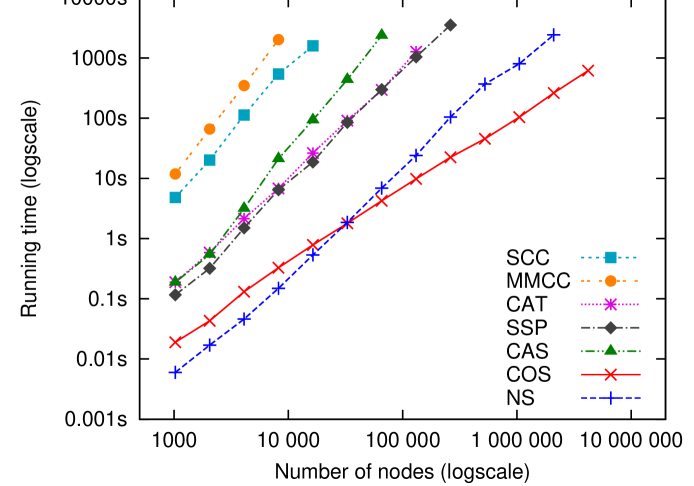
NETGEN-SR family ()
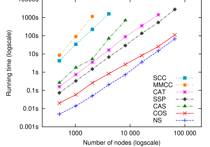
| SCC | MMCC | CAT | SSP | CAS | COS | NS | ||
|---|---|---|---|---|---|---|---|---|
| 8 | 4.81 | 11.85 | 0.19 | 0.12 | 0.19 | 0.02 | 0.01 | |
| 8 | 112.40 | 347.47 | 2.14 | 1.50 | 3.15 | 0.13 | 0.05 | |
| 8 | 1587.01 | 26.36 | 18.66 | 93.14 | 0.78 | 0.54 | ||
| 8 | 295.05 | 298.95 | 2360.21 | 4.24 | 6.88 | |||
| 8 | 3514.72 | 22.40 | 104.69 | |||||
| 8 | 103.83 | 799.26 | ||||||
| 8 | 615.42 |
| SCC | MMCC | CAT | SSP | CAS | COS | NS | ||
|---|---|---|---|---|---|---|---|---|
| 32 | 34.03 | 90.82 | 0.74 | 0.33 | 1.79 | 0.06 | 0.01 | |
| 45 | 224.79 | 1158.92 | 3.54 | 1.49 | 5.27 | 0.26 | 0.05 | |
| 64 | 1592.62 | 16.36 | 6.77 | 70.35 | 0.83 | 0.21 | ||
| 91 | 88.13 | 29.16 | 697.47 | 2.68 | 0.73 | |||
| 128 | 353.23 | 136.17 | 8.28 | 3.55 | ||||
| 181 | 1419.60 | 535.57 | 25.74 | 14.90 | ||||
| 256 | 2799.34 | 111.55 | 67.29 |
Table 5 contains performance results for the NETGEN-LO-8 family. As one would expect, these instances turned out to be easier to solve than NETGEN-8 instances of the same size. For this family, SSP was an order of magnitude faster than CAT, while CAS was even more efficient than the SSP algorithm by a factor between 2 and 3. Note that the relative performance of SSP and CAS is entirely different compared to the NETGEN-8 results. Nevertheless, the fastest methods were COS and NS just like for the NETGEN-8 family and their relationship was similar.
| SCC | MMCC | CAT | SSP | CAS | COS | NS | ||
|---|---|---|---|---|---|---|---|---|
| 8 | 0.82 | 2.52 | 0.14 | 0.02 | 0.01 | 0.01 | 0.00 | |
| 8 | 8.49 | 79.93 | 1.88 | 0.13 | 0.06 | 0.07 | 0.02 | |
| 8 | 73.83 | 1801.08 | 22.10 | 1.29 | 0.67 | 0.43 | 0.19 | |
| 8 | 668.00 | 183.06 | 17.79 | 6.67 | 2.65 | 2.11 | ||
| 8 | 2062.12 | 172.63 | 60.16 | 13.79 | 29.00 | |||
| 8 | 1342.73 | 519.06 | 68.41 | 293.49 | ||||
| 8 | 457.02 | 2482.50 |
Table 6 shows how the running time of the algorithms depends on the density of the network. NS was clearly the most efficient algorithm in these tests. COS and SSP were also relatively fast, while CAT turned out to be significantly slower and the other methods were not competitive. The CAS algorithm performed much worse than SSP on the dense instances.
| SCC | MMCC | CAT | SSP | CAS | COS | NS | ||
|---|---|---|---|---|---|---|---|---|
| 2 | 18.43 | 60.71 | 1.03 | 0.33 | 0.27 | 0.08 | 0.02 | |
| 8 | 112.40 | 347.47 | 2.14 | 1.50 | 3.15 | 0.13 | 0.05 | |
| 32 | 657.29 | 2655.80 | 7.41 | 4.40 | 35.54 | 0.43 | 0.13 | |
| 128 | 3523.55 | 32.03 | 12.73 | 273.76 | 1.98 | 0.39 | ||
| 512 | 147.58 | 35.58 | 2473.16 | 7.72 | 1.31 | |||
| 2048 | 624.44 | 99.49 | 47.08 | 6.68 |
Figure 2 and Tables 7 and 8 present the benchmark results for the GOTO families. These problems indeed turned out to be much harder than the NETGEN instances and the relative performance of the algorithms was also rather different than in case of the NETGEN families. Generally, COS and NS were the most efficient to solve these GOTO problems. COS was clearly the best method for the largest instances, even for the relatively dense GOTO-SR networks, which did not hold for the NETGEN-SR instances. Another notable difference compared to the NETGEN families is that CAS was orders of magnitude faster than SSP. It was quite efficient on GOTO-8 instances, although its performance was not stable. Among the cycle-canceling algorithms, CAT was clearly the most efficient similarly to the NETGEN problems. However, MMCC was 3-4 times faster than SCC, which is in contrast to the previous results.
GOTO-8 family ()
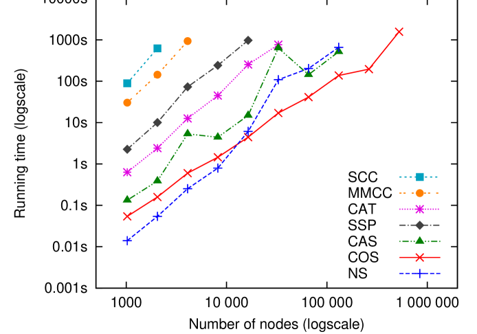
GOTO-SR family ()
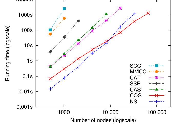
| SCC | MMCC | CAT | SSP | CAS | COS | NS | ||
|---|---|---|---|---|---|---|---|---|
| 8 | 88.85 | 30.39 | 0.63 | 2.27 | 0.13 | 0.05 | 0.01 | |
| 8 | 931.54 | 12.62 | 72.93 | 5.34 | 0.60 | 0.25 | ||
| 8 | 253.54 | 971.03 | 14.87 | 4.43 | 6.11 | |||
| 8 | 143.92 | 41.27 | 202.47 | |||||
| 8 | 195.36 | |||||||
| 8 |
| SCC | MMCC | CAT | SSP | CAS | COS | NS | ||
|---|---|---|---|---|---|---|---|---|
| 32 | 2474.46 | 584.35 | 2.30 | 35.66 | 2.81 | 0.30 | 0.08 | |
| 45 | 13.08 | 393.00 | 22.20 | 1.36 | 0.41 | |||
| 64 | 89.15 | 143.35 | 5.27 | 3.16 | ||||
| 91 | 415.69 | 1101.38 | 18.23 | 13.87 | ||||
| 128 | 2650.95 | 69.37 | 163.37 | |||||
| 181 | 358.44 | 1180.26 | ||||||
| 256 | 1279.72 |
Table 9 presents the results obtained for the ROAD family. As one would expect, the SSP algorithm was by far the fastest on these special instances. Our implementation of the CAS algorithm implies that it works exactly the same as SSP on this family since all capacities are set to one. Therefore, CAS is skipped in Table 9. The COS and NS algorithms performed an order of magnitude worse than SSP, while the cycle-canceling algorithms were drastically slower.
| SCC | MMCC | CAT | SSP | COS | NS | ||
|---|---|---|---|---|---|---|---|
| 9 559 | 3.11 | 2.29 | 372.91 | 2.17 | 0.01 | 0.14 | 0.04 |
| 49 109 | 2.46 | 37.25 | 47.65 | 0.10 | 1.47 | 0.69 | |
| 116 920 | 2.27 | 150.84 | 264.52 | 0.26 | 4.61 | 2.97 | |
| 261 155 | 2.38 | 1984.30 | 1373.49 | 0.96 | 15.23 | 14.14 | |
| 519 157 | 2.44 | 3.29 | 35.87 | 41.38 | |||
| 1 048 506 | 2.53 | 5.32 | 94.32 | 129.04 | |||
| 2 073 870 | 2.49 | 21.99 | 238.57 | 744.36 |
Finally, the performance results for the VISION family are presented in Table 10. We do not report running time for SCC and MMCC as they could not solve these problems within the timeout limit of one hour. COS performed clearly the best in these tests with the only exception of the first instance. Similarly to other families, the asymptotic behavior of NS was clearly worse than that of COS. CAS was superior to SSP, while CAT was even slower than SSP.
| CAT | SSP | CAS | COS | NS | ||
|---|---|---|---|---|---|---|
| 245 762 | 5.82 | 630.25 | 265.25 | 124.89 | 23.96 | 21.06 |
| 491 522 | 5.85 | 2304.01 | 970.49 | 622.22 | 61.25 | 108.64 |
| 983 042 | 5.88 | 1998.27 | 186.42 | 531.59 | ||
| 1 949 698 | 5.91 | 535.36 | 3420.76 | |||
| 3 899 394 | 5.92 | 1475.95 |
Recall from Sections 3.3 and 3.4 that the COS and NS algorithms have several variants. These variants were also compared systematically to determine the default options. Here we only present a representative selection of these results.
Tables 11 and 12 compare the variants of the COS algorithm on the NETGEN-8 and GOTO-8 families, respectively. COS-PR denotes the push-relabel variant, COS-AR denotes the augment-relabel variant, while COS denotes the partial augment-relabel variant, which is the default implementation. This latter technique was clearly faster than the other two approaches on all kinds of problem instances. The COS-AR variant performed similarly to COS-PR on some easy instances, such as the NETGEN-8 family, but was an order of magnitude slower on some other instances, such as the GOTO networks. These results show that COS-AR is not so robust than the other two methods, which is in accordance with Goldberg’s experiments in the maximum flow context [34].
| COS-PR | COS-AR | COS | ||
|---|---|---|---|---|
| 8 | 0.03 | 0.02 | 0.02 | |
| 8 | 0.17 | 0.14 | 0.13 | |
| 8 | 0.94 | 1.11 | 0.78 | |
| 8 | 6.37 | 5.72 | 4.24 | |
| 8 | 35.17 | 28.00 | 22.40 | |
| 8 | 176.87 | 179.13 | 103.83 | |
| 8 | 1064.62 | 901.07 | 615.42 |
| COS-PR | COS-AR | COS | ||
|---|---|---|---|---|
| 8 | 0.10 | 0.16 | 0.05 | |
| 8 | 0.89 | 2.48 | 0.60 | |
| 8 | 7.60 | 33.34 | 4.43 | |
| 8 | 78.55 | 911.05 | 41.27 | |
| 8 | 342.75 | 195.36 |
We implemented five pivot rules for the NS method, which significantly affect the efficiency of the algorithm. Tables 13 and 14 compare the overall performance of these strategies on the NETGEN-8 and GOTO-8 families, respectively. BE, FE, BS, CL, and AL denote the best eligible, first eligible, block search, candidate list, and altering candidate list pivot rules, respectively. These results and many other experiments show that the BS and AL rules are generally the most efficient. On GOTO instances, the FE and CL rules also performed similarly to these methods, but they were much slower in other cases, for example, on NETGEN instances. Since the BS rule turned out to be slightly more robust than AL, it was selected to be the default pivot strategy in our implementation. The BE rule resulted in the worst performance although it yielded less iterations than the other rules.
| NS-BE | NS-FE | NS-BS | NS-CL | NS-AL | ||
|---|---|---|---|---|---|---|
| 8 | 0.20 | 0.01 | 0.01 | 0.01 | 0.01 | |
| 8 | 3.40 | 0.14 | 0.05 | 0.06 | 0.04 | |
| 8 | 60.47 | 3.64 | 0.54 | 1.02 | 0.47 | |
| 8 | 1285.91 | 117.99 | 6.88 | 27.68 | 6.41 | |
| 8 | 104.69 | 808.10 | 98.97 | |||
| 8 | 799.26 | 800.36 |
| NS-BE | NS-FE | NS-BS | NS-CL | NS-AL | ||
|---|---|---|---|---|---|---|
| 8 | 0.50 | 0.01 | 0.01 | 0.01 | 0.02 | |
| 8 | 9.59 | 0.43 | 0.25 | 0.25 | 0.28 | |
| 8 | 151.92 | 6.84 | 6.11 | 5.90 | 6.16 | |
| 8 | 3024.80 | 251.48 | 202.47 | 216.21 | 220.16 |
4.3 Comparison to other solvers
The implementations presented in this paper were also compared to the following widely known MCF solvers. These codes were compiled using the same compiler and optimization level as we used for our implementations. The experiments were conducted using the default options of these solvers.
-
•
CS2. This is an authoritative implementation of the cost-scaling push-relabel algorithm. It was written by A.V. Goldberg and B. Cherkassky applying all improvements and heuristics described in [33]. CS2 has been widely used as a benchmark for solving the MCF problem for a long time. We used the latest version, CS2 4.6, which is available from the IG Systems, Inc. [16].
-
•
LEDA. This is a comprehensive C++ library [54], which also provides an MCF solver in its MIN_COST_FLOW() procedure. This method implements the cost-scaling push-relabel algorithm, as well. We used version 5.0 of the LEDA library in our experiments. In fact, LEDA 5.1.1 was also tested, but it turned out to be slower than version 5.0.
-
•
MCFZIB. This is the MCF code written by A. Löbel [57] at the Zuse Institute Berlin (ZIB). We denote this code as MCFZIB in order to differentiate it from the problem itself (similarly to the MCFClass project [27]). This solver features both a primal and a dual network simplex implementation, from which the former one is used by default as it is usually more efficient. We used the latest version 1.3, which is available at [58].
-
•
RelaxIV. This is a C++ translation of an authoritative implementation of the relaxation algorithm. The original FORTRAN code was written by D.P. Bertsekas and P. Tseng [8] and is available at [7]. The C++ translation was made by A. Frangioni and C. Gentile at the University of Pisa and is available as part of the MCFClass project [27]. This project provides a common C++ interface for several MCF solvers. Apart from RelaxIV, it also features CS2 and MCFZIB, but not their latest versions, thus we used these two solvers directly.
Our codes are part of an open source C++ optimization library, LEMON, which is available at http://lemon.cs.elte.hu/.
Tables 15, 16, 17, and 18 compare our implementations to the other four solvers on the NETGEN instances. As before, all codes were executed with a timeout limit of one hour and the average running time over three different random instances is reported for each problem size (in seconds). Our COS code performed similarly to CS2 on NETGEN-8 and NETGEN-SR families, while it was slightly slower on the other two NETGEN families. The solver of the LEDA library was about two times slower than these cost-scaling codes. Furthermore, it failed to solve the largest instances due to a number overflow error, which is denoted as “error” in the tables. Since LEDA has closed source, we could not eliminate this problem by replacing the number types used by the algorithm with larger ones. MCFZIB was typically slower than our NS code by a factor between 2 and 10, but they performed similarly on the NETGEN-LO-8 instances. RelaxIV was very efficient on these families. It was typically faster than all other codes for the largest instances, while NS was the most efficient on the smaller networks and on the NETGEN-DEG family.
| LEMON | Other implementations | ||||||||
|---|---|---|---|---|---|---|---|---|---|
| COS | NS | CS2 | LEDA | MCFZIB | RelaxIV | ||||
| 8 | 0.02 | 0.01 | 0.02 | 0.03 | 0.02 | 0.01 | |||
| 8 | 0.13 | 0.05 | 0.11 | 0.17 | 0.14 | 0.06 | |||
| 8 | 0.78 | 0.54 | 0.78 | 1.45 | 1.75 | 0.54 | |||
| 8 | 4.24 | 6.88 | 4.22 | 8.34 | 18.78 | 3.58 | |||
| 8 | 22.40 | 104.69 | 20.81 | error | 207.29 | 13.19 | |||
| 8 | 103.83 | 799.26 | 103.25 | error | 2985.08 | 89.90 | |||
| 8 | 615.42 | 566.32 | error | 419.38 | |||||
| LEMON | Other implementations | ||||||||
|---|---|---|---|---|---|---|---|---|---|
| COS | NS | CS2 | LEDA | MCFZIB | RelaxIV | ||||
| 32 | 0.06 | 0.01 | 0.05 | 0.08 | 0.05 | 0.03 | |||
| 45 | 0.26 | 0.05 | 0.18 | 0.38 | 0.20 | 0.26 | |||
| 64 | 0.83 | 0.21 | 0.59 | 1.41 | 0.68 | 1.30 | |||
| 91 | 2.68 | 0.73 | 2.04 | 5.07 | 3.28 | 1.94 | |||
| 128 | 8.28 | 3.55 | 7.86 | 19.61 | 21.68 | 4.53 | |||
| 181 | 25.74 | 14.90 | 29.00 | 72.48 | 111.74 | 13.98 | |||
| 256 | 111.55 | 67.29 | 104.25 | 274.06 | 634.38 | 44.37 | |||
| LEMON | Other implementations | ||||||||
|---|---|---|---|---|---|---|---|---|---|
| COS | NS | CS2 | LEDA | MCFZIB | RelaxIV | ||||
| 8 | 0.01 | 0.00 | 0.01 | 0.02 | 0.01 | 0.01 | |||
| 8 | 0.07 | 0.02 | 0.07 | 0.11 | 0.06 | 0.04 | |||
| 8 | 0.43 | 0.19 | 0.42 | 0.93 | 0.62 | 0.57 | |||
| 8 | 2.65 | 2.11 | 2.26 | 6.48 | 4.09 | 2.67 | |||
| 8 | 13.79 | 29.00 | 10.56 | error | 28.31 | 18.73 | |||
| 8 | 68.41 | 293.49 | 54.48 | error | 258.99 | 62.23 | |||
| 8 | 457.02 | 2482.50 | 299.15 | error | 2309.26 | 229.67 | |||
| LEMON | Other implementations | ||||||||
|---|---|---|---|---|---|---|---|---|---|
| COS | NS | CS2 | LEDA | MCFZIB | RelaxIV | ||||
| 2 | 0.08 | 0.02 | 0.04 | 0.08 | 0.05 | 0.04 | |||
| 8 | 0.13 | 0.05 | 0.11 | 0.17 | 0.14 | 0.06 | |||
| 32 | 0.43 | 0.13 | 0.31 | 0.70 | 0.42 | 0.37 | |||
| 128 | 1.98 | 0.39 | 1.12 | 2.91 | 1.32 | 1.40 | |||
| 512 | 7.72 | 1.31 | 5.15 | 12.56 | 4.74 | 3.20 | |||
| 2048 | 47.08 | 6.68 | 32.72 | 69.55 | 18.52 | 12.81 | |||
The performance results for the GOTO families are presented in Figure 3 and Tables 19 and 20. In these tests, COS and CS2 also performed similarly and they were the most efficient on the largest instances of both families. LEDA was also similarly efficient on GOTO-8 networks, but it was 2-3 times slower than CS2 and COS on the GOTO-SR family. NS turned out to be orders of magnitude faster than the other network simplex implementation, MCFZIB. Similarly to the NETGEN families, NS was the most efficient algorithm on the relatively small GOTO instances, but was substantially slower than the cost-scaling codes on the large networks. RelaxIV turned out to be very slow on these hard instances, which is in sharp contrast to its efficiency on the NETGEN instances.
GOTO-8 family ()
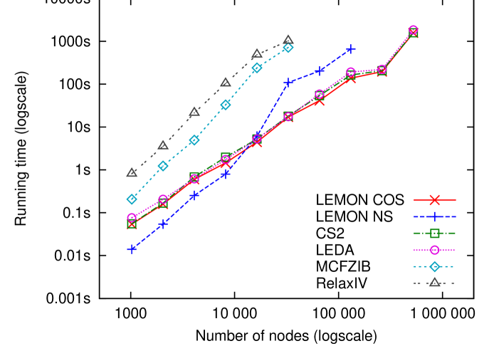
GOTO-SR family ()
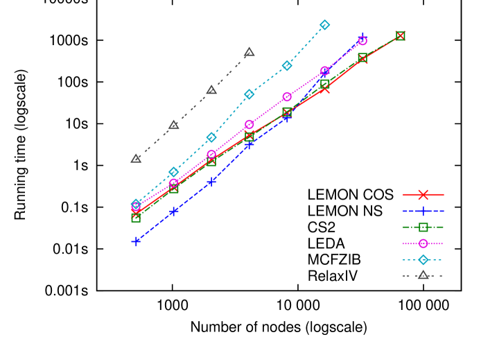
| LEMON | Other implementations | ||||||||
|---|---|---|---|---|---|---|---|---|---|
| COS | NS | CS2 | LEDA | MCFZIB | RelaxIV | ||||
| 8 | 0.05 | 0.01 | 0.06 | 0.08 | 0.21 | 0.81 | |||
| 8 | 0.60 | 0.25 | 0.69 | 0.62 | 4.94 | 21.29 | |||
| 8 | 4.43 | 6.11 | 5.23 | 5.24 | 239.67 | 487.23 | |||
| 8 | 41.27 | 202.47 | 54.05 | 58.50 | |||||
| 8 | 195.36 | 206.48 | 221.14 | ||||||
| 8 | |||||||||
| LEMON | Other implementations | ||||||||
|---|---|---|---|---|---|---|---|---|---|
| COS | NS | CS2 | LEDA | MCFZIB | RelaxIV | ||||
| 32 | 0.30 | 0.08 | 0.28 | 0.38 | 0.70 | 8.81 | |||
| 45 | 1.36 | 0.41 | 1.23 | 1.83 | 4.70 | 60.89 | |||
| 64 | 5.27 | 3.16 | 4.78 | 9.57 | 50.65 | 492.38 | |||
| 91 | 18.23 | 13.87 | 19.16 | 44.24 | 246.38 | ||||
| 128 | 69.37 | 163.37 | 89.32 | 184.97 | 2339.57 | ||||
| 181 | 358.44 | 1180.26 | 385.14 | 973.49 | |||||
| 256 | 1279.72 | 1259.63 | |||||||
Table 21 presents the results for the ROAD family. In this case, we also report the running time of our SSP implementation since it was by far the most efficient method for this special family. Apart from SSP, CS2 was typically the fastest to solve these instances. COS was slower than CS2 by a factor of at most two, while LEDA failed to solve the large instances due to overflow errors. NS and MCFZIB were significantly slower than CS2 and COS on the large networks. RelaxIV performed much worse than the other algorithms.
| LEMON | Other implementations | |||||||||
|---|---|---|---|---|---|---|---|---|---|---|
| SSP | COS | NS | CS2 | LEDA | MCFZIB | RelaxIV | ||||
| 9 559 | 3.11 | 0.01 | 0.14 | 0.04 | 0.12 | 0.14 | 0.14 | 0.58 | ||
| 49 109 | 2.46 | 0.10 | 1.47 | 0.69 | 0.84 | 1.07 | 1.62 | 22.41 | ||
| 116 920 | 2.27 | 0.26 | 4.61 | 2.97 | 2.67 | 3.19 | 6.09 | 168.03 | ||
| 261 155 | 2.38 | 0.96 | 15.23 | 14.14 | 7.53 | error | 27.25 | 2051.20 | ||
| 519 157 | 2.44 | 3.29 | 35.87 | 41.38 | 19.26 | error | 81.07 | |||
| 1 048 506 | 2.53 | 5.32 | 94.32 | 129.04 | 49.73 | error | 197.54 | |||
| 2 073 870 | 2.49 | 21.99 | 238.57 | 744.36 | 131.90 | error | 992.32 | |||
The benchmark results for the VISION family are presented in Table 22. In these tests, CS2 was clearly the most efficient and COS was about 1.5 times slower than it. All other algorithms performed significantly worse, including the third cost-scaling code, LEDA. NS was superior to MCFZIB and LEDA, but was less efficient than CS2 and COS for the large networks. Similarly to the GOTO and ROAD instances, RelaxIV was much slower than the other solvers.
| LEMON | Other implementations | ||||||||
|---|---|---|---|---|---|---|---|---|---|
| COS | NS | CS2 | LEDA | MCFZIB | RelaxIV | ||||
| 245 762 | 5.82 | 23.96 | 21.06 | 19.78 | 54.62 | 131.66 | 904.74 | ||
| 491 522 | 5.85 | 61.25 | 108.64 | 44.18 | 207.51 | 333.20 | 3518.20 | ||
| 983 042 | 5.88 | 186.42 | 531.59 | 139.05 | 1250.56 | ||||
| 1 949 698 | 5.91 | 535.36 | 3420.76 | 348.28 | |||||
| 3 899 394 | 5.92 | 1475.95 | 916.47 | ||||||
Finally, on behalf of a brief overview of our experiments, Table 23 presents running time results for one representation of each problem family. Those instances were selected that have about two million arcs. The first part of the table contains running time in seconds, while the second part reports normalized time results. In the cases when the execution of an algorithm reached the timeout limit of one hour, we report a lower bound on the ratio by which it would have been slower than the fastest implementation.
| Running time | |||||||||
|---|---|---|---|---|---|---|---|---|---|
| LEMON | Other implementations | ||||||||
| Family | COS | NS | CS2 | LEDA | MCFZIB | RelaxIV | |||
| NETGEN-8 | 2 097 152 | 22.40 | 104.69 | 20.81 | error | 207.29 | 13.19 | ||
| NETGEN-SR | 2 097 152 | 8.28 | 3.55 | 7.86 | 19.61 | 21.68 | 4.53 | ||
| NETGEN-LO-8 | 2 097 152 | 13.79 | 29.00 | 10.56 | error | 28.31 | 18.73 | ||
| NETGEN-DEG | 2 097 152 | 7.72 | 1.31 | 5.15 | 12.56 | 4.74 | 3.20 | ||
| GOTO-8 | 2 097 152 | 195.36 | 206.48 | 221.14 | |||||
| GOTO-SR | 2 097 152 | 69.37 | 163.37 | 89.32 | 184.97 | 2339.57 | |||
| ROAD | 2 653 624 | 94.32 | 129.04 | 49.73 | error | 197.54 | |||
| VISION | 2 877 382 | 61.25 | 108.64 | 44.18 | 207.51 | 333.20 | 3518.20 | ||
| Normalized time | |||||||||
| LEMON | Other implementations | ||||||||
| Family | COS | NS | CS2 | LEDA | MCFZIB | RelaxIV | |||
| NETGEN-8 | 2 097 152 | 1.70 | 7.94 | 1.58 | error | 15.72 | 1.00 | ||
| NETGEN-SR | 2 097 152 | 2.33 | 1.00 | 2.21 | 5.52 | 6.11 | 1.28 | ||
| NETGEN-LO-8 | 2 097 152 | 1.31 | 2.75 | 1.00 | error | 2.68 | 1.77 | ||
| NETGEN-DEG | 2 097 152 | 5.89 | 1.00 | 3.93 | 9.59 | 3.62 | 2.44 | ||
| GOTO-8 | 2 097 152 | 1.00 | 18 | 1.06 | 1.13 | 18 | 18 | ||
| GOTO-SR | 2 097 152 | 1.00 | 2.36 | 1.29 | 2.67 | 33.73 | 52 | ||
| ROAD | 2 653 624 | 1.90 | 2.59 | 1.00 | error | 3.97 | 38 | ||
| VISION | 2 877 382 | 1.39 | 2.46 | 1.00 | 4.70 | 7.54 | 79.63 | ||
Table 23 as well as the previous results clearly demonstrate that CS2 and COS are the most robust implementations and NS is the third one in terms of the overall performance. MCFZIB is considerably slower than NS, but it is still robust. LEDA performed well in several cases, but it often failed to solve the large instances due to numerical problems. RelaxIV is not robust at all as it turned out to be much slower than the other implementations on all problem families except for the NETGEN networks.
5 Conclusions
In this paper, we have considered the minimum-cost flow (MCF) problem and various solution methods along with experiments with their efficient implementations. The MCF problem plays a fundamental role in network flow theory and has a wide range of applications. Therefore, efficient implementations of MCF algorithms are essential in practice.
We implemented several algorithms for solving the MCF problem and thoroughly experimented with many variants of them as well as with various practical improvements and heuristics. This work provides insight into these details and gives some guidelines for implementing the considered algorithms efficiently. An interesting novel result is the application of Goldberg’s recent partial augment-relabel idea [34] in the cost-scaling algorithm, which turned out to be a significant improvement. Another widely used efficient algorithm is the network simplex method, which was implemented using a quite efficient data structure and various pivot strategies. Moreover, three cycle-canceling algorithms and two augmenting path algorithms were also implemented.
An extensive experimental evaluation was carried out to compare these algorithms. In general, the cost-scaling (COS) and the network simplex (NS) methods turned out to be the most efficient and the most robust. On relatively small instances (up to a few thousands of nodes), NS was clearly the fastest algorithm. However, COS significantly outperformed it on the largest networks due to its better asymptotic behavior in terms of the number of nodes. We also remark that NS usually performed better than other methods on rather dense networks, most likely because it is based on maintaining a spanning tree data structure and the tree update process depends only on the number of the nodes. Apart from COS and NS, the other algorithms usually performed worse and it turned out that their relative performance greatly depends on the characteristics of the problem instance. In certain cases, if the flow need not be split into many paths, however, the augmenting path algorithms are superior to other methods.
The presented implementations were systematically compared to publicly available efficient MCF solvers, as well. It turned out that our cost-scaling code is substantially more efficient and more robust than that of the LEDA library [54] and it performs similarly to or slightly slower than CS2 [33, 16], which is an authoritative implementation of this algorithm. Our implementation of the network simplex method turned out to be significantly faster than the other considered implementation of this algorithm, the MCF solver [57, 58]. Furthermore, another well-known MCF solver, RelaxIV [8, 7, 27] was also tested, but it did not turn out to be robust at all. It was orders of magnitude slower than the other codes on various problem families, although it was rather efficient on particular instances (namely, the NETGEN problems).
Our implementations are not standalone solvers, but they are part of a versatile C++ network optimization library, LEMON [55, 21] (http://lemon.cs.elte.hu/). Therefore, these codes have the additional advantage that they can easily be combined with various practical data structures and powerful algorithms related to network optimization. Furthermore, LEMON is an open source library that can be used in both commercial and non-commercial software development under a permissive license. The authors believe that this library with its great variety of efficient algorithms is a viable alternative to the MCFClass project [27], which features several publicly available MCF solvers under a common C++ interface.
Finally, we remark some ideas for future work. First, our implementation of the cost-scaling algorithm currently does not incorporate the speculative arc fixing heuristic, which was suggested by Goldberg [33]. We believe that the efficiency of this implementation could be further improved by also applying this complicated technique. Furthermore, a more comprehensive experimental study could be carried out considering more problem families and more publicly available implementations of MCF algorithms.
Acknowledgements
The authors are grateful to A.V. Goldberg and B. Cherkassky, D.P. Bertsekas and P. Tseng, and A. Löbel for developing CS2, RelaxIV, and MCF codes, respectively and for making these solvers available for academic use. We thank A. Frangioni and C. Gentile for developing the MCFClass project including the C++ translation of the RelaxIV solver, which was used in our experiments. We also thank A. Frangioni for his help in using the MCFClass project. Furthermore, we are grateful to A. Jüttner and B. Dezső for their useful suggestions related to the presented implementations.
Research was supported by grants (no. CNK 77780 and no. CK 80124) from the National Development Agency of Hungary, based on a source from the Research and Technology Innovation Fund, and by TÁMOP grant 4.2.1/B-09/1/KMR-2010-0003.
References
- [1] R.K. Ahuja, A.V. Goldberg, J.B. Orlin, R.E. Tarjan, Finding minimum-cost flows by double scaling, Math. Program. 53 (1992) 243–266.
- [2] R.K. Ahuja, T.L. Magnanti, J.B. Orlin, Network flows, in: G.L. Nemhauser, A.H.G. Rinnooy Kan, M.J. Todd (eds), Handbooks in Operations Research and Management Science, Vol. 1, pp. 211–369. Elsevier, 1989.
- [3] R.K. Ahuja, T.L. Magnanti, J.B. Orlin, Network Flows: Theory, Algorithms, and Applications, Prentice-Hall, Inc., 1993.
- [4] F. Barahona, É. Tardos, Note on Weintraub’s minimum-cost circulation algorithm, SIAM J. Comput. 18 (1989) 579–583.
- [5] R.S. Barr, F. Glover, D. Klingman, Enhancements to spanning tree labelling procedures for network optimization, INFOR 17 (1979) 16–34.
- [6] D.P. Bertsekas, A distributed algorithm for the assignment problem, Working Paper, Laboratory for Information and Decision Systems, MIT, Cambridge, MA, 1979.
- [7] D.P. Bertsekas, Network Optimization Codes, http://web.mit.edu/dimitrib/www/noc.htm, 1994.
- [8] D.P. Bertsekas, P. Tseng, RELAX-IV: A faster version of the relax code for solving minimum cost flow problems, Technical Report LIDS-P-2276, Dept. of Electrical Engineering and Computer Science, MIT, Cambridge, MA, 1994.
- [9] R.G. Bland, D.L. Jensen. On the computational behavior of a polynomial-time network flow algorithm, Math. Program. 54 (1982) 1–39.
- [10] G. Bradley, G. Brown, G. Graves, Design and implementation of large scale primal transshipment algorithms, Manag. Sci. 24 (1977) 1–34.
- [11] U. Bünnagel, B. Korte, J. Vygen, Efficient implementation of the Goldberg-Tarjan minimum-cost flow algorithm, Opt. Methods and Software 10 (1998) 157–174.
- [12] R.G. Busacker, P.J. Gowen, A procedure for determining a family of minimum-cost network flow patterns, Technical Report ORO-TP-15, Operations Research Office, The Johns Hopkins University, Bethesda, MD, 1960.
- [13] R.G. Busacker, T.L. Saaty, Finite Graphs and Networks: An Introduction with Applications, McGraw-Hill, New York, NY, 1965.
- [14] COIN-OR – Computational Infrastructure for Operations Research. http://www.coin-or.org/, 2012.
- [15] T.H. Cormen, C.E. Leiserson, R.L. Rivest, C. Stein, Introduction to Algorithms, The MIT Press, 3rd edition, 2009.
- [16] CS2 Software, Version 4.6. IG Systems, Inc., http://www.igsystems.com/cs2/, 2009.
- [17] W.H. Cunningham, Theoretical properties of the network simplex method, Math. Oper. Res. 4 (1979) 196–208.
- [18] G.B. Dantzig, Linear Programming and Extensions, Princeton University Press, Princeton, NJ, 1963.
- [19] A. Dasdan, Experimental analysis of the fastest optimum cycle ratio and mean algorithms, ACM Trans. Des. Autom. Electron. Syst. 9 (2004) 385–418.
- [20] A. Dasdan, R.K. Gupta, Faster maximum and minimum mean cycle algorithms for system performance analysis, IEEE Trans. Computer-Aided Design 17 (1998) 889–899.
- [21] B. Dezső, A. Jüttner, P. Kovács, LEMON – an open source C++ graph template library, Electron. Notes Theor. Comput. Sci. 264 (2011) 23–45.
- [22] DIMACS, Network Flows and Matching: First DIMACS Implementation Challenge, FTP site: ftp://dimacs.rutgers.edu/pub/netflow/, 2012.
- [23] DIMACS. Shortest Paths: Ninth DIMACS Implementation Challenge, WWW site: http://www.dis.uniroma1.it/~challenge9/, 2012.
- [24] J. Edmonds, R.M. Karp, Theoretical improvements in algorithmic efficiency for network flow problems, J. ACM 19 (1972) 248–264.
- [25] MTA-ELTE Egerváry Research Group on Combinatorial Optimization (EGRES), http://www.cs.elte.hu/egres/, 2012.
- [26] L.R. Ford, D.R. Fulkerson, Flows in Networks, Princeton University Press, Princeton, NJ, 1962.
- [27] A. Frangioni, C. Gentile, The MCFClass Project, http://www.di.unipi.it/di/groups/optimize/Software/MCF.html, 2011.
- [28] A. Frangioni, A. Manca, A computational study of cost reoptimization for min-cost flow problems, INFORMS J. Comput. 18 (2006) 61–70.
- [29] A. Frank, Connections in Combinatorial Optimization, Oxford Lecture Series in Mathematics and Its Applications, Vol. 38. Oxford University Press, 2011.
- [30] H.N. Gabow, R.E. Tarjan, Faster scaling algorithms for network problems, SIAM J. Comput. 18 (1989) 1013–1036.
- [31] L. Georgiadis, A.V. Goldberg, R.E. Tarjan, R.F. Werneck, An experimental study of minimum mean cycle algorithms, In I. Finocchi, J. Hershberger, editors, Proc. 6th International Workshop on Algorithm Engineering and Experiments, ALENEX 2009, pp 1–13, New York, NY, 2009. SIAM.
- [32] A.V. Goldberg, Scaling algorithms for the shortest paths problem, SIAM J. Comput. 24 (1995) 494–504.
- [33] A.V. Goldberg, An efficient implementation of a scaling minimum-cost flow algorithm, J. Algorithms 22, 1 1–29.
- [34] A.V. Goldberg, The partial augment-relabel algorithm for the maximum flow problem. In Proc. 16th Annual European Symposium on Algorithms, ESA ’08, pp. 466–477, Heidelberg, Germany, 2008. Springer-Verlag.
- [35] A.V. Goldberg, M. Kharitonov, On implementing scaling push-relabel algorithms for the minimum-cost flow problem, In D.S. Johnson, C.C. McGeoch (eds.) Network Flows and Matching: First DIMACS Implementation Challenge, DIMACS Series in Discrete Mathematics and Theoretical Computer Science, Vol. 12, pp. 157–198. AMS, 1993.
- [36] A.V. Goldberg, R.E. Tarjan, A new approach to the maximum-flow problem, J. ACM 35 (1988) 921–940.
- [37] A.V. Goldberg, R.E. Tarjan. Finding minimum-cost circulations by canceling negative cycles, J. ACM 36 (1989) 873–886.
- [38] A.V. Goldberg, R.E. Tarjan. Finding minimum-cost circulations by successive approximation. Math. Oper. Res. 15 (1990) 430–466.
- [39] D. Goldfarb, J. Hao, Polynomial simplex algorithms for the minimum cost network flow problem, Algorithmica 8 (1992) 145–160.
- [40] D. Goldfarb, J. Hao, S.-R. Kai, Anti-stalling pivot rules for the network simplex algorithm, Networks 20 (1990) 79–91.
- [41] M.D. Grigoriadis, An efficient implementation of the network simplex method, Math. Program. Stud. 26 (1986) 83–111.
- [42] M. Hartmann, J.B. Orlin, Finding minimum cost to time ratio cycles with small integral transit times, Networks 23 (1993) 567–574.
- [43] R.A. Howard, Dynamic Programming and Markov Processes, The MIT Press, 1960.
- [44] M. Iri, A new method for solving transportation-network problems, J. Oper. Res. Soc. Japan 3 (1960) 27–87.
- [45] W.S. Jewell, Optimal flow through networks, Technical Report Interim Technical Report No. 8, Operations Research Center, MIT, Cambridge, MA, 1958.
- [46] R.M. Karp, A characterization of the minimum cycle mean in a digraph, Discrete Math. 23 (1978) 309–311.
- [47] D.J. Kelly, G.M. O’Neill, The minimum cost flow problem and the network simplex solution method, Master’s thesis, University College, Dublin, 1991.
- [48] J.L. Kennington, R.V. Helgason, Algorithms for Network Programming, John Wiley & Sons, Inc., New York, NY, 1980.
- [49] Z. Király, P. Kovács, An experimental study of minimum cost flow algorithms, Proc. 8th International Conference on Applied Informatics, Vol. 2., pp 227–235, Eger, Hungary, 2010.
- [50] M. Klein, A primal method for minimal cost flows with applications to the assignment and transportation problems, Manag. Sci. 14 (1967) 205–220.
- [51] D. Klingman, A. Napier, J. Stutz, NETGEN: A program for generating large scale capacitated assignment, transportation, and minimum cost flow network problems, Manag. Sci. 20 (1974) 814–821.
- [52] B. Korte and J. Vygen, Combinatorial Optimization: Theory and Algorithms, Algorithms and Combinatorics, Vol. 21. Springer-Verlag, 5th edition, 2012.
- [53] H.W. Kuhn, The Hungarian Method for the assignment problem, Naval Res. Logist. Quart. 2 (1955) 83–97.
- [54] The LEDA library, Version 5.0. Algorithmic Solutions Software GmbH, http://www.algorithmic-solutions.com/leda/, 2004.
- [55] LEMON – Library for Efficient Modeling and Optimization in Networks, http://lemon.cs.elte.hu/, 2012.
- [56] LEMON Documentation, Version 1.2.3, http://lemon.cs.elte.hu/pub/doc/1.2.3/, 2012.
- [57] A. Löbel, Solving large-scale real-world minimum-cost flow problems by a network simplex method, Technical Report SC 96-7, Zuse Institute Berlin (ZIB), Berlin, Germany, 1996.
- [58] A. Löbel, MCF Version 1.3 – A network simplex implementation. www.zib.de, 2004.
- [59] J.M. Mulvey. Pivot strategies for primal-simplex network codes. J. ACM 25 (1978) 266–270.
- [60] J.B. Orlin, A faster strongly polynomial minimum cost flow algorithm, Oper. Res. 41 (1993) 338–350.
- [61] J.B. Orlin, A polynomial time primal network simplex algorithm for minimum cost flows, Math. Program. 78 (1997) 109–129.
- [62] J.B. Orlin, S.A. Plotkin, É. Tardos, Polynomial dual network simplex algorithms, Math. Program. 60 (1993) 255–276 1993.
- [63] H. Röck. Scaling techniques for minimal cost network flows, In U. Pape, editor, Discrete Structures and Algorithms, pp. 181–191, München, 1980. Carl Hanser.
- [64] A. Schrijver, Combinatorial Optimization: Polyhedra and Efficiency, Algorithms and Combinatorics, Vol. 24. Springer-Verlag, 2003.
- [65] D.D. Sleator, R.E. Tarjan, A data structure for dynamic trees, J. Comput. System Sci. 26 (1983) 362–391.
- [66] P.T. Sokkalingam, R.K. Ahuja, J.B. Orlin, New polynomial-time cycle-canceling algorithms for minimum-cost flows, Networks 36 (2000) 53–63.
- [67] É. Tardos, A strongly polynomial minimum cost circulation algorithm, Combinatorica 5 (1985) 247–255.
- [68] R.E. Tarjan, Efficiency of the primal network simplex algorithm for the minimum-cost circulation problem, Math. Oper. Res. 16 (1991) 272–291.
- [69] R.E. Tarjan, Dynamic trees as search trees via euler tours, applied to the network simplex algorithm, Math. Program. 78 (1997) 169–177.
- [70] N. Tomizawa, On some techniques useful for solution of transportation network problems, Networks 1 (1971) 173–194.
Received: March 15, 2012 Revised: May 20, 2012