Convergence of linear functionals of the Grenander estimator under misspecification

Abstract

Under the assumption that the true density is decreasing, it is well known that the Grenander estimator converges at rate $n^{1/3}$ if the true density is curved [Sankhyā Ser. A 31 (1969) 23–36] and at rate $n^{1/2}$ if the density is flat [Ann. Probab. 11 (1983) 328–345; Canad. J. Statist. 27 (1999) 557–566]. In the case that the true density is misspecified, the results of Patilea [Ann. Statist. 29 (2001) 94–123] tell us that the global convergence rate is of order $n^{1/3}$ in Hellinger distance. Here, we show that the local convergence rate is $n^{1/2}$ at a point where the density is misspecified. This is not in contradiction with the results of Patilea [Ann. Statist. 29 (2001) 94–123]: the global convergence rate simply comes from locally curved well-specified regions. Furthermore, we study global convergence under misspecification by considering linear functionals. The rate of convergence is $n^{1/2}$ and we show that the limit is made up of two independent terms: a mean-zero Gaussian term and a second term (with nonzero mean) which is present only if the density has well-specified locally flat regions.

t1Supported in part by an NSERC Discovery Grant.

1 Introduction

Shape-constrained nonparametric maximum likelihood estimators provide an intriguing alternative to kernel-based density estimators. For example, one can compare the standard histogram with the Grenander estimator for a decreasing density. Rules exist to pick the bandwidth (or bin width) for the histogram to attain optimal convergence rates, cf. Wasserman (2006). On the other hand, the Grenander estimator gives a piecewise constant density, or histogram, but the bin widths are now chosen completely automatically by the estimator. Furthermore, the bin widths selected by the Grenander estimator are naturally locally adaptive [Birgé (1987); Cator (2011)]. Similar comparisons can also be made between the log-concave nonparametric MLE and the kernel density estimator with, say, the Gaussian kernel.

The Grenander estimator was first introduced in Grenander (1956) and has been considered extensively in the literature since then. A recent review of the history of the problem appears in Durot, Kulikov and Lopuhaä (2012). The latter paper establishes that the Grenander estimator converges to a true strictly decreasing density at a rate of $(n/\log n)^{1/3}$ in the $L_{\infty}$ norm. Other rates have also been derived over the years, most notably, convergence at a point at a rate of $n^{1/3}$ if the true density is locally strictly decreasing [Prakasa Rao (1969); Groeneboom (1985)] and at a rate of $n^{1/2}$ if the true density is locally flat [Groeneboom (1983); Carolan and Dykstra (1999)].

As noted in Cule, Samworth and Stewart (2010); Dümbgen, Samworth and Schuhmacher (2011), the “success story” of maximum likelihood estimators is their robustness. Namely, let $\mathcal{F}$ denote the space of decreasing densities on ${\mathbb{R}}_{+}$. Next, let $f_{0}$ denote the true density and $\hat{f}_{0}$ denote the density closest to $f_{0}$ in the Kullback–Leibler sense. That is,

$$\hat{f}_{0}=\mathop{\operatorname{argmin}}_{g\in\mathcal{F}}\int_{0}^{\infty}f_{0}(x)\log\frac{f_{0}(x)}{g(x)}\,dx.$$ (1)

We will call the density $\hat{f}_{0}$ the KL projection density of $f_{0}$, or the KL projection for short. Note that if $f_{0}\in\mathcal{F}$ then $\hat{f}_{0}=f_{0}$. Patilea (2001) showed that the density $\hat{f}_{0}$ exists, and that the Grenander estimator converges to $\hat{f}_{0}$ when the observed samples come from the true density $f_{0}$, regardless if $f_{0}\in\mathcal{F}$. Similar results were proved for the log-concave maximum likelihood estimator in Cule and Samworth (2010); Cule, Samworth and Stewart (2010); Dümbgen, Samworth and Schuhmacher (2011); Balabdaoui et al. (2013).

In order to understand the local behavior of the Grenander estimator when $f_{0}\notin\mathcal{F}$, we first need to define regions where $f_{0}$ is considered to be miss- and well-specified. Let $\widehat{F}_{0}$ denote the cumulative distribution function of $\hat{f}_{0}$ defined in (1). The regions where $\widehat{F}_{0}\neq F_{0}$ are then the regions where $f_{0}$ is misspecified, and $f_{0}$ is considered to be well specified otherwise. Note that, if $f_{0}$ is misspecified in a region, it may still be decreasing on some portion of this region; see, for example, Figure 1.

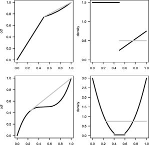
Figure 1: Two examples of $f_{0}$ and $\hat{f}_{0}=\operatorname{gren}(F_{0})$. The two left panels show the c.d.f. and density, for example, (4) while the two right panels show the c.d.f. and density, for example, (5). $F_{0}$ (resp., $f_{0}$) is shown in black, and $\widehat{F}_{0}$ (resp., $\hat{f}_{0}$) is shown in gray, but only if different from the truth (namely $F_{0}$ and $f_{0}$, resp.).

Let $\hat{f}_{n}$ denote the Grenander estimator of a decreasing density. We show here that at a point where the density is misspecified the rate of convergence of $\hat{f}_{n}$ to $\hat{f}_{0}$ is $n^{1/2}$, and we also identify the limiting distribution. This is not in contradiction with the results of Patilea (2001): the slower $n^{1/3}$ global convergence rate simply comes from locally curved well-specified regions. To be more specific, if the density $f_{0}$ is misspecified at a point, then $\widehat{F}_{0}$ must be linear (and $\hat{f}_{0}$ is flat), and in regions where $\hat{f}_{0}$ is flat the rate of convergence is $n^{1/2}$. In fact, the $n^{1/2}$ rate holds at all flat regions of $\hat{f}_{0}$, irrespective of whether these are miss- or well-specified. The complete result is given in Section 2, where some properties of $\hat{f}_{0}$ are also discussed.

Next, we consider convergence of linear functionals. Let

$$\hat{\mu}_{0}(g)=\int_{0}^{\infty}g(x)\hat{f}_{0}(x)\,dx\quad\mbox{and}\quad\hat{\mu}_{n}(g)=\int_{0}^{\infty}g(x)\hat{f}_{n}(x)\,dx.$$ (2)

In Section 3, we show that $n^{1/2}(\hat{\mu}_{n}(g)-\hat{\mu}_{0}(g))=O_{p}(1)$, and we again identify the limiting distribution. Notably, the limit is made up of two independent terms: a mean-zero Gaussian term and a second term with nonzero mean. Furthermore, the second term is present only if the density has well-specified locally flat regions. Our results apply to a wide range of KL projections with both strictly curved and flat regions. The work in the strictly curved case follows from the rates of convergence of $\widehat{F}_{n}(y)=\int_{0}^{y}\hat{f}_{n}(y)\,dy$ to the empirical distribution function established in Kiefer and Wolfowitz (1976). However, as mentioned above, this is only for the well-specified regions of $f_{0}$. A related work here is that of Kulikov and Lopuhaä (2008), who consider functionals in the strictly curved case but at the distribution function level.

In Section 4, we go beyond the linear setting, and consider convergence of the entropy functional in the misspecified case. The limit in this case is Gaussian, irrespective of the local properties of $\hat{f}_{0}$. Most proofs appear in Section 6 and some technical details are given in Jankowski (2014). Throughout, our results are illustrated by reproducible simulations. Code for these is available online at www.math.yorku.ca/ hkj/.

To our best knowledge, previous work on rates of convergence under misspecification in the shape-constrained context is limited to the rates established in van de Geer (2000) and Patilea (2001), as well as the more recent results of Balabdaoui et al. (2013). In Balabdaoui et al. (2013), the pointwise asymptotic distribution under misspecification was derived for the log-concave probability mass function.

The implications of the new results obtained here are as follows. First, we now understand that $\hat{f}_{0}$ will be made up of local well specified and misspecified regions, and that the rate of convergence in the misspecified regions is always $n^{1/2}$. We conjecture that this type of behavior will be seen in other situations, such as the log-concave setting for $d=1$. That is, the rate of convergence in misspecified regions will be $n^{1/2}$ whereas in well-specified regions the rate of convergence will depend on whether locally the density lies on the boundary or the interior of the underlying space. In the log-concave $d=1$ case, this “interior” rate is known to be $n^{2/5}$ [Balabdaoui, Rufibach and Wellner (2009)]. The interesting case of $d>1$ is more mysterious though, as the relationship between the slower boundary points and faster interior points is harder to identify.

Secondly, we show that linear functionals (as well as the nonlinear entropy functional) converge at rate $n^{1/2}$, and we also conjecture that this behavior will continue to hold for other shape constraints. Let $\mu_{0}(g)=\int_{0}^{\infty}g(x)f_{0}(x)\,dx$. Our results show that

$$\sqrt{n}\bigl{(}\hat{\mu}_{n}(g)-\mu_{0}(g)\bigr{)}=O_{p}(1)+\sqrt{n}\bigl{(}\hat{\mu}_{0}(g)-\mu_{0}(g)\bigr{)}.$$ (3)

Therefore, global rates of divergence are $n^{1/2}$ for linear functionals in the misspecified case. A similar statement also holds for the entropy functional, and here the random $O_{p}(1)$ term is always Gaussian. Such results are well understood in parametric settings, and are key in power calculations. The exact conditions necessary for (3) to hold are given in Section 3 for $\mu_{0}(g)$ and in Section 4 for the entropy. Our work can also be easily extended to locally misspecified settings such as those studied in Le Cam (1960).

Lastly, the fact that the limiting distribution of the linear functional $\hat{\mu}_{n}(g)$ depends on properties of $\hat{f}_{0}$, whereas the limiting distribution of the entropy functional is always Gaussian, makes the entropy functional potentially more appealing in terms of testing procedures. Hypothesis testing based on functionals was considered, for example, in Cule, Samworth and Stewart (2010) and Chen and Samworth (2013). The latter reference develops the “trace test” which depends on a nearly linear functional, the variance. Both, however, are developed in the context of log-concavity, and it would be of great interest to extend the results presented here to that setting, particularly for higher dimensions.

2 The Kullback–Leibler projection and pointwise convergence under misspecification

Properties of the KL projection onto the space of log-concave densities were studied in Dümbgen, Samworth and Schuhmacher (2011). When projecting onto the space of decreasing densities, the behavior is a little easier to characterize.

Theorem 2.1 ([Patilea (1997, 2001)])

Let $f_{0}$ be a density with support on $[0,\infty)$ with $F_{0}(x)=\int_{0}^{x}f_{0}(u)\,du$. Let $\widehat{F}_{0}$ denote the least concave majorant of $F_{0}$. Then the left derivative of $\widehat{F}_{0},\hat{f}_{0}$, satisfies the inequality $\int\log\frac{\hat{f}_{0}}{f}\,dF_{0}\geq 0$, for all decreasing densities $f$.

Remark 2.2.

The density $\hat{f}_{0}$ satisfying $\int\log\frac{\hat{f}_{0}}{f}\,dF_{0}\geq 0$ for all $f\in\mathcal{F}$ is called the “pseudo-true” density by Patilea (2001). If we additionally assume that $\sup_{f\in\mathcal{F}}\int\log f\,dF_{0}$ and $\int\log f_{0}\,dF_{0}$ are both finite, then this $\hat{f}_{0}$ is also the unique minimizer of the Kullback–Leibler divergence

$$\hat{f}_{0}=\mathop{\operatorname{argmin}}_{f\in\mathcal{F}}\int\log\frac{f_{0}}{f}\,dF_{0}.$$

See Patilea (2001), page 95, for more details. In what follows, we continue to refer to $\hat{f}_{0}$ as defined in Theorem 2.1, as the KL projection, even if it comes from the slightly more general definition of Patilea (2001).

Thus, in our setting, we have a complete graphical representation of the distribution function $\widehat{F}_{0}$ of the KL projection. This representation makes it possible to calculate $\hat{f}_{0}$ in many cases. It also allows us to easily visualize the various $F_{0}$ which yield the same $\hat{f}_{0}$. Moreover, the representation is key in understanding the behavior of the estimator, both on the finite sample and asymptotic levels. Therefore, for a function $g$ we define the operator $\operatorname{gren}(g)$ to denote the (left) derivative of the least concave majorant of $g$. When the least concave majorant is restricted to a set $[a,b]$, we will write $\operatorname{gren}_{[a,b]}(g)$.

Let $\mathcal{S}_{0}$ denote the support of $f_{0}$. We write $\mathcal{S}_{0}=\mathcal{M}\cup\mathcal{W}$, where $\mathcal{M}=\{x\geq 0\dvtx\widehat{F}_{0}(x)>F_{0}(x)\}$ and $\mathcal{W}=\{x\geq 0\dvtx\widehat{F}_{0}(x)=F_{0}(x)\}$. Since $f_{0}$ is a density, it follows that $F_{0}$ is continuous, as is $\widehat{F}_{0}$ and, therefore, $\mathcal{W}$ is a closed set and $\mathcal{M}$ is open. For a fixed point $x_{0}\in\mathcal{M}$, we thus know that $x_{0}$ lies in some open interval. Indeed, let $a_{0}=\sup\{x<x_{0}\dvtx\widehat{F}_{0}(x)=F_{0}(x)\}$ and $b_{0}=\inf\{x>x_{0}\dvtx\widehat{F}_{0}(x)=F_{0}(x)\}$. Then $x_{0}\in(a_{0},b_{0})$ with $(a_{0},b_{0})\subset\mathcal{M}$.

Two examples are given in Figure 1. For the first example, we have

$$f_{0}(x) = \cases{1.5,&\quad$x\in[0,0.5]$,\vspace*{2pt}\cr x-0.25,&\quad$x\in(0.5,1]$.}$$ (4)

Here, $\mathcal{M}=(0.5,1)$ and $\mathcal{W}=[0,0.5]\cup\{1\}$. For the second example, we have

$$f_{0}(x) = \cases{12(x-0.5)^{2},&\quad$x\in[0,0.4]\cup[0.6,1]$,\vspace*{2pt}\cr 0.04,&\quad$x\in(0.4,0.6)$.}$$ (5)

Here, $\mathcal{M}=(0.25,1)$ and $\mathcal{W}=[0,0.25]\cup\{1\}$.

The next proposition gives some additional properties of the KL projection.

Proposition 2.3

The density, $\hat{f}_{0}$, satisfies the following: [(2)]

Fix $x_{0}\in\mathcal{M}$ and define $a_{0},b_{0}$ as above. Then $b_{0}<\infty$, and $\hat{f}_{0}$ is constant on $(a_{0},b_{0}]$ and satisfies the mean-value property

$$\hat{f}_{0}(x_{0})=\frac{1}{b_{0}-a_{0}}\int_{a_{0}}^{b_{0}}f_{0}(x)\,dx.$$

Suppose that $\int_{0}^{\infty}f_{0}^{2}(x)\,dx<\infty$. Then

$$\hat{f}_{0}=\mathop{\operatorname{argmin}}_{g\in\mathcal{F}}\int_{0}^{\infty}\bigl{(}g(x)-f_{0}(x)\bigr{)}^{2}\,dx.$$

For any increasing function $h(x)$, $\int_{0}^{\infty}h(x)\hat{f}_{0}(x)\,dx\leq\int_{0}^{\infty}h(x)f_{0}(x)\,dx$.

Let $g_{0}\in\mathcal{F}$ and let $G_{0}(y)=\int_{0}^{y}g_{0}(x)\,dx$. Then

$$\sup_{x\geq 0}\bigl{|}\widehat{F}_{0}(x)-G_{0}(x)\bigr{|} \leq \sup_{x\geq 0}\bigl{|}F_{0}(x)-G_{0}(x)\bigr{|}.$$

Point (3) above tells us that if $g$ is increasing then $\mu_{0}(g)\geq\hat{\mu}_{0}(g)$. Point (4) is Marshall’s lemma [Marshall (1970)]. The proof of Proposition 2.3 appears in Jankowski (2014).

Suppose that $X_{1},\ldots,X_{n}$ are independent and identically distributed with density $f_{0}$ on ${\mathbb{R}}_{+}=[0,\infty)$. Let $\hat{f}_{n}$ denote the Grenander estimator of a decreasing density

$$\hat{f}_{n}=\mathop{\operatorname{argmax}}_{g\in\mathcal{F}}\int\log g(x)\,d{\mathbb{F}}_{n}(x),$$

where $\mathcal{F}$ denotes the class of decreasing densities on ${\mathbb{R}}_{+}$, and ${\mathbb{F}}_{n}(x)=n^{-1}\sum_{i=1}^{n}1_{(-\infty,x]}(X_{i})$ denotes the empirical distribution function. The next theorem is our first main result.

Theorem 2.4

Fix a point $x_{0}\in\mathcal{M}$, and let $[a,b]$ denote the largest interval $I$ containing $x_{0}$ such that $\widehat{F}_{0}(x)$ is linear on $I$. Let ${\mathbb{U}}$ denote a standard Brownian bridge process on $[0,1]$, and let ${\mathbb{U}}_{F_{0}}(x)={\mathbb{U}}(F_{0}(x))$ for $x\in\mathcal{S}_{0}$. Then

$$\sqrt{n}\bigl{(}\hat{f}_{n}(x_{0})-\hat{f}_{0}(x_{0})\bigr{)} \Rightarrow \operatorname{gren}_{[a,b]}\bigl{(}{\mathbb{U}}^{\mathrm{mod}}_{F_{0}}\bigr{)}(x_{0}),$$

where

$${\mathbb{U}}^{\mathrm{mod}}_{F_{0}}(u) = \cases{{\mathbb{U}}_{F_{0}}(u),&\quad$u\in[a,b]\cap\mathcal{W}$,\vspace*{2pt}\cr-\infty,&\quad$u\in[a,b]\cap\mathcal{M}$.}$$

If it happens that $[a,b]\cap\mathcal{W}=\{a,b\}$, then

$$\sqrt{n}\bigl{(}\hat{f}_{n}(x_{0})-\hat{f}_{0}(x_{0})\bigr{)} \Rightarrow \sigma Z,$$

where $Z$ is a standard normal random variable and

$$\sigma^{2} = \hat{f}_{0}(x_{0})\biggl{[}\frac{1}{b-a}-\hat{f}_{0}(x_{0})\biggr{]}.$$

Recall that Patilea (2001), Corollary 5.6, shows that the rate of convergence (in Hellinger distance) of $\hat{f}_{n}$ to $\hat{f}_{0}$ is $n^{1/3}$. The above theorem shows that the local rate of convergence will be $\sqrt{n}$ where the KL projection is flat. When the KL density is curved, the KL density and true density are actually equal, and hence the convergence rate from the correctly specified case applies. The next formulation of the limiting process is similar to that of Carolan and Dykstra (1999) for a density with a flat region on $[a,b]$.

Remark 2.5.

Let $p_{0}=F_{0}(b)-F_{0}(a)=\widehat{F}_{0}(b)-\widehat{F}_{0}(a)$. Since $\widehat{F}_{0}$ is linear on $[a,b]$ the limiting distribution may also be expressed as

$$\operatorname{gren}_{[a,b]}\bigl{(}{\mathbb{U}}^{\mathrm{mod}}_{F_{0}}\bigr{)}(x_{0}) = \frac{1}{b-a}\biggl{\{}Z+\sqrt{p_{0}}\operatorname{gren}\bigl{(}{\mathbb{U}}^{\mathrm{mod}}\bigr{)}\biggl{(}\frac{x_{0}-a}{b-a}\biggr{)}\biggr{\}},$$

where $Z$ is a mean zero normal random variable with variance $p_{0}(1-p_{0})$, ${\mathbb{U}}$ is an independent standard Brownian bridge, and

$${\mathbb{U}}^{\mathrm{mod}}(u) = \cases{{\mathbb{U}}(u),&\quad$u\in\bigl{(}[a,b]\cap\mathcal{W}-a\bigr{)}/(b-a)$,\vspace*{2pt}\cr-\infty,&\quad$u\in\bigl{(}[a,b]\cap\mathcal{M}-a\bigr{)}/(b-a)$.}$$

Notably, if $[a,b]\cap\mathcal{W}=\{a,b\}$, then $\operatorname{gren}({\mathbb{U}}^{\mathrm{mod}})(u)=0$.

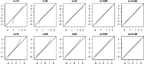
Figure 2: Empirical quantiles of $\sqrt{n}(\hat{f}_{n}(x_{0})-\hat{f}_{0}(x_{0}))$ vs. the true quantiles of the limiting $N(0,\sigma^{2})$ distributions at the point $x_{0}=0.75$ for $f_{0}$ given by (4) in the top row ($\sigma^{2}=3/4)$ and (5) in the bottom row ($\sigma^{2}=7/16$). The sample size varies from $n=10$ to $n={}$100,000. The straight line goes through the origin and has slope one. Each plot is based on $B=1000$ samples.

Figure 2 illustrates the theory. The convergence is surprisingly fast, although it appears to be a little slower in the second example (5). We conjecture that this difference is caused by the presence/absence of the strictly curved region of $f_{0}$.

Proof of Theorem 2.4 By the switching relation [Balabdaoui et al. (2011)], we have

$$P\bigl{(}\sqrt{n}\bigl{(}\hat{f}_{n}(x_{0})-\hat{f}_{0}(x_{0})\bigr{)}<t\bigr{)}$$

$$\qquad=P\Bigl{(}\mathop{\operatorname{argmax}}_{z\geq 0}\bigl{\{}{\mathbb{F}}_{n}(z)-\bigl{(}\hat{f}_{0}(x_{0})+n^{-1/2}t\bigr{)}z\bigr{\}}<x\Bigr{)}$$

$$\qquad=P\Bigl{(}\mathop{\operatorname{argmax}}_{z\geq 0}\bigl{\{}\sqrt{n}\bigl{(}{\mathbb{F}}_{n}(z)-{\mathbb{F}}_{n}(a)-\bigl{(}F_{0}(z)-F_{0}(a)\bigr{)}\bigr{)}$$

$$\hskip 83.0pt{}+\sqrt{n}\bigl{(}F_{0}(z)-F_{0}(a)-\hat{f}_{0}(x_{0})(z-a)\bigr{)}-tz\bigr{\}}<x\Bigr{)}.$$

We now look more closely at the “second” term. That is,

$$F_{0}(z)-F_{0}(a)-\hat{f}_{0}(x_{0})(z-a)$$

$$\qquad=-\bigl{\{}\widehat{F}_{0}(z)-F_{0}(z)\bigr{\}}+\bigl{\{}\widehat{F}_{0}(z)-\widehat{F}_{0}(a)-\hat{f}_{0}(x_{0})(z-a)\bigr{\}},$$

noting that $\widehat{F}_{0}(a)=F_{0}(a)$, since $a\in[a,b]\cap\mathcal{W}$. On the other hand, for all $z\in[a,b]\cap\mathcal{M}$, we have $\widehat{F}_{0}(z)>F_{0}(z)$. Furthermore, $\widehat{F}_{0}$ is concave with derivative $\hat{f}_{0}(x_{0})$ [at any point $z\in(a,b)$], and hence

$$\widehat{F}_{0}(z)-\widehat{F}_{0}(a)-\hat{f}_{0}(x_{0})(z-a)\leq 0$$

for all $z\geq 0$. For $z\in[a,b]\cap\mathcal{W}$ this is an equality, and a strict inequality otherwise. Therefore, the weak limit of

$$\sqrt{n}\bigl{\{}{\mathbb{F}}_{n}(z)-{\mathbb{F}}_{n}(a)-\bigl{(}F_{0}(z)-F_{0}(a)\bigr{)}\bigr{\}}-\sqrt{n}\bigl{(}F_{0}(z)-F_{0}(a)-\hat{f}_{0}(x_{0})(z-a)\bigr{)}$$

is ${\mathbb{U}}_{F_{0}}^{\mathrm{mod}}(z)-{\mathbb{U}}_{F_{0}}^{\mathrm{mod}}(a)={\mathbb{U}}_{F_{0}}^{\mathrm{mod}}(z)-{\mathbb{U}}_{F_{0}}(a)$, for all $z\in[a,b]$. For $z\notin[a,b]\cap\mathcal{W}$, the limit of this process is always $-\infty$ and, therefore, the maximum must occur inside of $[a,b]$. By the argmax continuous mapping theorem [van der Vaart and Wellner (1996), Theorem 3.2.2, page 287],

$$P\bigl{(}\sqrt{n}\bigl{(}\hat{f}_{n}(x_{0})-\hat{f}_{0}(x_{0})\bigr{)}<t\bigr{)}$$

$$\qquad\rightarrow P\Bigl{(}\mathop{\operatorname{argmax}}_{z\in[a,b]}\bigl{\{}{\mathbb{U}}_{F_{0}}^{\mathrm{mod}}(z)-tz\bigr{\}}<x\Bigr{)}=P\bigl{(}\operatorname{gren}_{[a,b]}\bigl{(}{\mathbb{U}}_{F_{0}}^{\mathrm{mod}}\bigr{)}(x_{0})<t\bigr{)}$$

by switching again. When $[a,b]\cap\mathcal{W}=\{a,b\}$, then the least concave majorant is simply the line joining ${\mathbb{U}}_{F_{0}}(a)$ and ${\mathbb{U}}_{F_{0}}(b)$, with slope equal to

$$\frac{{\mathbb{U}}_{F_{0}}(b)-{\mathbb{U}}_{F_{0}}(a)}{b-a},$$

a Gaussian random variable with mean zero and variance

$$\frac{1}{(b-a)^{2}}\bigl{(}F_{0}(b)-F_{0}(a)\bigr{)}\bigl{[}1-\bigl{(}F_{0}(b)-F_{0}(a)\bigr{)}\bigr{]}$$

$$\qquad=\hat{f}_{0}(x_{0})\biggl{[}\frac{1}{b-a}-\hat{f}_{0}(x_{0})\biggr{]}.$$

Proof of Remark 2.5 Recall that $\widehat{F}_{0}$ is linear on $[a,b]$. Therefore, for $x\in[a,b]$, we can write ${\mathbb{U}}(\widehat{F}_{0}(x))-{\mathbb{U}}(\widehat{F}_{0}(a))=\frac{x-a}{b-a}{\mathbb{W}}+{\mathbb{V}}(x)$, where

$${\mathbb{W}} = {\mathbb{U}}\bigl{(}\widehat{F}_{0}(b)\bigr{)}-{\mathbb{U}}\bigl{(}\widehat{F}_{0}(a)\bigr{)},$$

$${\mathbb{V}}(x) = {\mathbb{U}}\bigl{(}\widehat{F}_{0}(x)\bigr{)}-{\mathbb{U}}\bigl{(}\widehat{F}_{0}(a)\bigr{)}-\frac{\widehat{F}_{0}(x)-\widehat{F}_{0}(a)}{\widehat{F}_{0}(b)-\widehat{F}_{0}(a)}{\mathbb{W}}$$

$$= {\mathbb{U}}\bigl{(}\widehat{F}_{0}(x)\bigr{)}-{\mathbb{U}}\bigl{(}\widehat{F}_{0}(a)\bigr{)}-\frac{x-a}{b-a}{\mathbb{W}}.$$

Since all variables are jointly Gaussian, a careful calculation of the covariances reveals that ${\mathbb{W}}$ and ${\mathbb{V}}(x)$ are independent (also as processes), and ${\mathbb{W}}$ is mean-zero Gaussian with variance $p_{0}(1-p_{0})$. Furthermore,

$${\mathbb{V}}(s)\stackrel{{\scriptstyle d}}{{=}}\sqrt{p_{0}}{\mathbb{U}}\biggl{(}\frac{s-a}{b-a}\biggr{)}.$$

This decomposition is similar to that of Shorack and Wellner (1986), Exercise 2.2.11, page 32. Now, note that the Grenander operator satisfies $\operatorname{gren}_{[a,b]}(g)(x)=\beta+\frac{\gamma}{b-a}\operatorname{gren}_{[0,1]}(h)(\frac{t-a}{b-a})$ if $g(t)=\alpha+\beta t+\gamma h(\frac{t-a}{b-a})$. It follows that

$$\operatorname{gren}_{[a,b]}({\mathbb{U}}_{\widehat{F}_{0}})(x_{0}) = \frac{1}{b-a}Z+\frac{\sqrt{p_{0}}}{b-a}\operatorname{gren}({\mathbb{U}})\biggl{(}\frac{x_{0}-a}{b-a}\biggr{)}$$

with $Z,{\mathbb{U}}$ defined as in the remark. The full result follows since, ${\mathbb{U}}^{\mathrm{mod}}_{F_{0}}(x)={\mathbb{U}}^{\mathrm{mod}}_{\widehat{F}_{0}}(x)=\frac{x-a}{b-a}{\mathbb{W}}+{\mathbb{V}}^{\mathrm{mod}}(x)$.

3 $\sqrt{n}$-convergence of linear functionals

Consider a density $f_{0}$ with support $\mathcal{S}_{0}$ and let $\hat{f}_{0}$ denote its KL projection. We write $\mathcal{S}_{0}=\mathcal{S}_{c}\cup\mathcal{S}_{f}$, where $\mathcal{S}_{c}$ denotes the portion of the support where $\hat{f}_{0}$ is curved and $\mathcal{S}_{f}$ denotes the portion of the support where $\hat{f}_{0}$ is flat. By definition of $S_{f}$ as well as Proposition 2.3, the KL projection can be written as

$$\hat{f}_{0}(x) = \sum_{j=1}^{J}\hat{q}_{j}1_{I_{j}}(x)$$ (6)

on $S_{f}$, where the intervals are disjoint and each is of the form $I_{j}=(a_{j},b_{j}]$. Our results for linear functionals hold under the following assumptions:

[(C)]

The support, $\mathcal{S}_{0}$, of $f_{0}$ is bounded.

When the KL projection is curved, $\sup_{x\in\mathcal{S}_{c}}|f^{\prime}_{0}(x)|<+\infty$.

The true density is strictly positive: $\inf_{x\in S_{0}}f_{0}(x)>0$.

When the KL projection is flat, $J$ is finite in (6). Let $g\dvtx\mathcal{S}_{0}\mapsto{\mathbb{R}}$ and define $\hat{\mu}_{n}(g)$ by (2). Then we require that $g$ satisfy the following conditions: [(G2)]

$\int_{\mathcal{S}_{c}}|g^{\prime}(x)|\,dx<\infty$.

$g\in L_{\beta}(\mathcal{S}_{f})$ for some $\beta>2$.

In order to state our main result for linear functionals, we need to define the following functions:

$$g_{j}(u) = g\bigl{(}(b_{j}-a_{j})u+a_{j}\bigr{)},\qquad u\in[0,1],$$

$$\bar{g}_{j} = (b_{j}-a_{j})^{-1}\int_{a_{j}}^{b_{j}}g(x)\,dx$$

and

$$\bar{g}(x)=\cases{g(x),&\quad$x\in\mathcal{S}_{c}$,\vspace*{2pt}\cr\bar{g}_{j},&\quad$x\in I_{j},j=1,\ldots,J$.}$$ (8)

Thus, $\bar{g}_{1},\ldots,\bar{g}_{J}$ are the local averages of the function $g$, and each $g_{j}(u)$ is a localized version of $g$.

Theorem 3.1

Suppose that the density $f_{0}$ satisfies conditions (S), (C), (P) and (F). Consider a function $g\dvtx\mathcal{S}_{0}\mapsto{\mathbb{R}}$ which satisfies conditions (G1) and (G2). Let ${\mathbb{U}},{\mathbb{U}}_{1},\ldots,{\mathbb{U}}_{J}$ denote independent Brownian bridges, ${\mathbb{U}}_{F_{0}}(x)={\mathbb{U}}(F_{0}(x))$, and define ${\mathbb{U}}_{j}^{\mathrm{mod}}$ as in Theorem 2.4. Then

$$\sqrt{n}\bigl{(}\hat{\mu}_{n}(g)-\hat{\mu}_{0}(g)\bigr{)} \Rightarrow \int_{\mathcal{S}_{0}}\bar{g}(x)\,d{\mathbb{U}}_{F_{0}}(x)$$

$${}+\sum_{j=1}^{J}\sqrt{p_{j}}\int_{0}^{1}g_{j}(u)\operatorname{gren}\bigl{(}{\mathbb{U}}_{j}^{\mathrm{mod}}\bigr{)}(u)\,du,$$

where $p_{j}=F_{0}(b_{j})-F_{0}(a_{j})=\widehat{F}_{0}(b_{j})-\widehat{F}_{0}(a_{j})$. Furthermore,

$$\int_{\mathcal{S}_{0}}\bar{g}(x)\,d{\mathbb{U}}_{F_{0}}(x)=\int_{\mathcal{S}_{0}}\bar{g}(x)\,d{\mathbb{U}}_{\widehat{F}_{0}}(x).$$

Also, if $I_{j}\cap\mathcal{W}=\{a_{j},b_{j}\}$, then $\operatorname{gren}({\mathbb{U}}_{j}^{\mathrm{mod}})\equiv 0$.

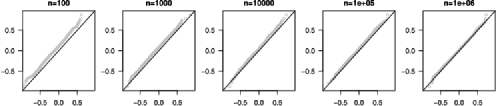
Figure 3: Empirical quantiles of $\sqrt{n}(\hat{\mu}_{n}(g)-\hat{\mu}_{0}(g))$ with $g(x)=x$ vs. the true quantiles of the limiting $N(0,\sigma^{2})$ distribution for $f_{0}$ given in (5), with $\sigma^{2}\approx 0.07032$.

It follows that $\sqrt{n}(\hat{\mu}_{n}(g)-\hat{\mu}_{0}(g))$ will converge to a Gaussian limit for true density (5) but not for (4), as the latter has well-specified flat regions. A simulation for (5) is shown in Figure 3. The proof of Theorem 3.1 is given in Section 6. The simulations show that there appears a systematic bias prior to convergence (the empirical quantiles appear on the $x$-axis in Figure 3, the negative bias translates to a left-shift in the plot). The proof of Proposition 6.1 shows that one source of the bias is the term $\sqrt{n}\int xd(\widehat{F}_{n}-{\mathbb{F}}_{n})\approx-\sqrt{n}\int(\widehat{F}_{n}-{\mathbb{F}}_{n})\leq 0$. When $\mathcal{S}_{0}=\mathcal{S}_{c}$, this term is the only source of bias, and from Kiefer and Wolfowitz (1976), it converges to zero at a rate of at least $n^{1/6}(\log n)^{-2/3}$. Since (3) of Proposition 2.3 also holds at the empirical level, similar behavior will be seen for all increasing functions $g$.

The results of Theorem 3.1 also show that $\sqrt{n}(\hat{\mu}_{n}(g)-\hat{\mu}_{0}(g))$ is asymptotically normal with variance $\operatorname{var}_{f_{0}}(\bar{g}(X))=\operatorname{var}_{\hat{f}_{0}}(\bar{g}(X))$ if $\mathcal{S}_{0}$ has no well-specified flat regions. Additionally, if $\mathcal{S}_{0}=\mathcal{S}_{c}$, then $\bar{g}(x)=g(x)$ and the model is well specified. In this case, $\hat{\mu}_{n}(g)$ has the same asymptotic distribution as the empirical estimator $n^{-1}\sum_{i=1}^{n}g(X_{i})$ (see also Proposition 6.1). This shows that the maximum likelihood estimator is asymptotically efficient, as in the strictly curved case the family of decreasing densities is complete, and hence the “naive estimator” $n^{-1}\sum_{i=1}^{n}g(X_{i})$ is asymptotically efficient [van de Geer (2003), Example 4.7].

Finally, we make a few comments on the assumptions required for Theorem 3.1 to hold. The assumptions which we use on $S_{c}$ are (S), (P) and (C). These are quite standard assumptions in the literature for the strictly curved setting; see, for example, Kiefer and Wolfowitz (1976); Durot, Kulikov and Lopuhaä (2012); Kulikov and Lopuhaä (2008); Groeneboom, Hooghiemstra and Lopuhaä (1999); Durot and Lopuhaä (2013). In the misspecified region, the required assumptions are (P) and (F). Note also that by Remark 3.2, the assumption (G2) is required in the result. Additional discussions of these assumptions, including directions for future research, are provided in the Jankowski (2014).

To further illustrate these assumptions, as well as Theorem 3.1, we consider the examples (4) and (5). In example (4), we have that

$$\hat{f}_{0}(x) = 1.5\,1_{[0,0.5]}(x)+0.5\,1_{(0.5,1]}(x).$$ (9)

The conditions (S) and (P) are clearly satisfied, as is (C) since $\mathcal{S}_{0}=\mathcal{S}_{f}$. Lastly, (F) holds with $J=2,\hat{q}_{1}=1.5,\hat{q}_{2}=0.5,I_{1}=(0,0.5],I_{2}=(0.5,1]$.Applying Theorem 3.1 for $g(x)=x$, we find that $\bar{g}(x)=0.75\,1_{[0,0.5]}(x)+\break 0.25\,1_{(0.5,1]}(x)$, and $I_{2}\cap\mathcal{W}=\{a_{2},b_{2}\}$ [hence $\operatorname{gren}({\mathbb{U}}^{\mathrm{mod}}_{2})=0$]. Therefore,

$$\sqrt{n}\bigl{(}\hat{\mu}_{n}(g)-\hat{\mu}_{0}(g)\bigr{)}$$

$$\qquad\Rightarrow\int_{0}^{1}\bar{g}(x)\,d{\mathbb{U}}_{F_{0}}(x)+\sqrt{\frac{3}{4}}\int_{0}^{1}\frac{u}{2}\operatorname{gren}\bigl{(}{\mathbb{U}}_{1}^{\mathrm{mod}}\bigr{)}(u)\,du$$

$$\qquad=-\frac{1}{2}{\mathbb{U}}_{F_{0}}(0.5)+\sqrt{\frac{3}{16}}\int_{0}^{1}u\operatorname{gren}({\mathbb{U}}_{1})(u)\,du,$$

where ${\mathbb{U}}_{F_{0}},{\mathbb{U}}_{1}$ are independent Brownian bridges as defined in Theorem 3.1. Notably, the limit has a non-Gaussian component.

Example (5) can be analyzed similarly. Here,

$$\hat{f}_{0}(x) = 12(x-0.5)^{2}1_{[0,0.25]}(x)+0.75\,1_{(0.25,1]}(x).$$

Again, the conditions (S) and (P) clearly hold. On $S_{c}=[0,0.25]$, we have $\sup_{x\in S_{c}}|f^{\prime}_{0}(x)|=12$ and, therefore, condition (C) holds. On $\mathcal{S}_{f}=(0.25,1]$ we have $J=1$, and hence (F) also holds. Applying Theorem 3.1 for $g(x)=x$, we find that $\bar{g}(x)=x1_{[0,0.25]}(x)+(5/8)1_{(0.25,1]}(x)$, and $I_{1}\cap\mathcal{W}=\{a_{1},b_{1}\}$ [hence $\operatorname{gren}({\mathbb{U}}^{\mathrm{mod}}_{1})=0$]. Therefore,

$$\sqrt{n}\bigl{(}\hat{\mu}_{n}(g)-\hat{\mu}_{0}(g)\bigr{)} \Rightarrow \int_{0}^{1}\bar{g}(x)\,d{\mathbb{U}}_{F_{0}}(x).$$

That is, the limit is zero-mean Gaussian with variance $\sigma^{2}\approx 0.07032$.

Remark 3.2.

Marginal properties of the process $\operatorname{gren}({\mathbb{U}})$ were studied in Carolan and Dykstra (2001). The results include marginal densities and moments, including $\mathrm{E}[(\operatorname{gren}({\mathbb{U}})(x))^{2}]=0.5(x^{2}/(1-x)+(1-x)^{2}/x)$. It follows that $\mathrm{E}[\int_{0}^{1}(\operatorname{gren}({\mathbb{U}})(x))^{2}\,dx]=\int_{0}^{1}(1-x)^{2}/x\,dx=\infty$, and hence the limiting process

$$\bigl{\langle}g,\operatorname{gren}({\mathbb{U}})\bigr{\rangle} = \int_{0}^{1}g(x)\operatorname{gren}({\mathbb{U}})(x)\,dx,$$

exists only for $g\in L_{\beta}(\mathcal{S}_{f})$ for $\beta>2$. We would therefore not expect convergence of $\hat{\mu}_{n}(g)$ for $g\in L_{\beta}(\mathcal{S}_{f})$ with $\beta\in[1,2]$.

4 Beyond linear functionals: A special case

Entropy measures theamount of disorder or uncertainty in a system and is closely related to the Kullback–Leibler divergence. Let $T(f)=\int_{0}^{\infty}f(x)\log f(x)\,dx$ denote the entropy functional. A review of testing and other applications of entropy appears, for example, in Beirlant et al. (1997).

Theorem 4.1

Suppose that $\hat{f}_{0}$ is bounded, the support of $f_{0}$ is also bounded, and that $f_{0}/\hat{f}_{0}\leq c_{0}^{2}<\infty$. Then

$$\sqrt{n}\bigl{(}T(\hat{f}_{n})-T(\hat{f}_{0})\bigr{)} \Rightarrow \sigma Z,$$

where $Z$ is a standard normal random variable and

$$\sigma^{2}=\operatorname{var}_{f_{0}}\bigl{(}\log\bigl{(}\hat{f}_{0}(X)\bigr{)}\bigr{)}=\operatorname{var}_{\hat{f}_{0}}\bigl{(}\log\bigl{(}\hat{f}_{0}(X)\bigr{)}\bigr{)}.$$

The proof is made up of two key pieces: (1) tight bounds on the likelihood ratio from Lemma 4.2 and (2) specialized equalities which hold for the Grenander estimator.

Lemma 4.2

Suppose that $\hat{f}_{0}$ is bounded, the support of $f_{0}$ is also bounded, and that $f_{0}/\hat{f}_{0}\leq c_{0}^{2}<\infty$. Then

$$\int\log\frac{\hat{f}_{n}}{\hat{f}_{0}}\,d{\mathbb{F}}_{n} = O_{p}\bigl{(}n^{-2/3}\bigr{)}.$$

We note that the conditions we require here are stronger than those of Patilea (2001), Corollary 5.6. However, under those conditions Patilea (2001) establishes convergence rates on $\int\log\frac{2\hat{f}_{n}}{\hat{f}_{n}+\hat{f}_{0}}\,d{\mathbb{F}}_{n}$, which is not sufficient for our purposes. The condition that $f_{0}/\hat{f}_{0}$ is bounded above was also used in the study of misspecification in van de Geer (2000), Section 10.4. The condition that the support of $f_{0}$ is bounded is the strongest, whereas the condition that $\hat{f}_{0}$ is bounded may be relaxed somewhat. We discuss this further in Jankowski (2014).

Proof of Lemma 4.2 We first show that $\int_{0}^{\infty}\varphi(\hat{f}_{n})\,d(\widehat{F}_{n}-{\mathbb{F}}_{n})=0$ for any function $\varphi$. This follows since $\widehat{F}_{n}(x)\geq{\mathbb{F}}_{n}(x)$ with equality at finitely many touch points, and also $\hat{f}_{n}$ is constant between all touch points. Thus, letting $\tau_{1},\tau_{2},\ldots,\tau_{m}$ enumerate the (random) points of touch, we have

$$\int_{0}^{\infty}\varphi(\hat{f}_{n})\,d(\widehat{F}_{n}-{\mathbb{F}}_{n}) = \sum_{i=1}^{m}\varphi\bigl{(}\hat{f}_{n}(\tau_{i})\bigr{)}\bigl{(}(\widehat{F}_{n}-{\mathbb{F}}_{n})(\tau_{i})-(\widehat{F}_{n}-{\mathbb{F}}_{n})(\tau_{i-1})\bigr{)}=0$$

with $\tau_{0}=0$ and $\tau_{m}=X_{(n)}$. A similar argument also establishes that

$$\int_{0}^{\infty}\varphi(\hat{f}_{0})\,d(\widehat{F}_{0}-F_{0})=\int_{\mathcal{M}}\varphi(\hat{f}_{0})\,d(\widehat{F}_{0}-F_{0})=0.$$ (11)

For $\varphi(v)=\log v$, it follows that

$$\sqrt{n}\bigl{(}T(\hat{f}_{n})-T(\hat{f}_{0})\bigr{)} = \sqrt{n}\biggl{(}\int\log\hat{f}_{n}\,d\widehat{F}_{n}-\int\log\hat{f}_{0}\,d\widehat{F}_{0}\biggr{)}$$

$$= \sqrt{n}\int\log\biggl{(}\frac{\hat{f}_{n}}{\hat{f}_{0}}\biggr{)}\,d{\mathbb{F}}_{n}+\sqrt{n}\int\log\hat{f}_{0}\,d({\mathbb{F}}_{n}-F_{0}).$$

The first term is $O_{p}(n^{-1/6})$ by Lemma 4.2. The second term has a Gaussian limit with variance $\operatorname{var}_{f_{0}}(\log\hat{f}_{0}(X))$. By (11) [with $\varphi(v)=\log^{2}v,\log v$] this is equal to $\operatorname{var}_{\hat{f}_{0}}(\log\hat{f}_{0}(X))$.

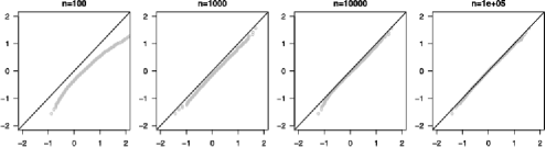
Figure 4: Empirical quantiles of $\sqrt{n}(T(\hat{f}_{n})-T(\hat{f}_{0}))$ vs. the true quantiles of the limiting $N(0,\sigma^{2})$ distribution for $f_{0}$ given in (4), with $\sigma^{2}\approx 0.2263$.

A simulation of this result is shown in Figure 4 based on the true density (4). The KL projection of (4) is given in (9). One can easily check that the conditions of Theorem 4.1 are satisfied in this case. Note that this density has well-specified flat regions and, therefore, linear functionals that do not ignore $\mathcal{S}_{f}\cap\mathcal{W}$ should have non-Gaussian terms in their limit; see, for example, (3) for the case when $g(x)=x$. On the other hand, the entropy functional will always result in a Gaussian limit. The simulations exhibit a systematic positive bias. The proof shown above reveals the cause: the term $\int\log({\hat{f}_{n}}/{\hat{f}_{0}})\,d{\mathbb{F}}_{n}\geq 0$ since $\hat{f}_{n}$ is the MLE. In the plots the quantiles of $\sqrt{n}(T(\hat{f}_{n})-T(\hat{f}_{0}))$ are shown on the $x$-axis, and these quantiles appear to be shifted to the right—that is, they are larger than the quantiles of the limiting Gaussian distribution.

5 Conclusion

We anticipate that extensions of this work to other one-dimensional shape-constrained models, such as the log-concave and convex decreasing constraints, are within reach, although certain technical difficulties will need to be overcome. In particular, the results of Patilea (2001) for convex models should yield some results for convex decreasing densities under misspecification. The Grenander estimator has a particular simplicity of form, which we have exploited here. Some progress for the log-concave setting has already been made in Balabdaoui et al. (2013), albeit for the discrete (i.e., probability mass function) setting. We conjecture that statements such as (3) will continue to hold for other shape-constraints in $d=1$ for linear functionals. Similar results for higher-dimensional shape-constrained models seem premature in view of the current lack of rate of convergence results even when the model is correctly specified.

6 Proofs for Section 3

We now present the proof for Theorem 3.1. We proceed by proving convergence results for the different types of behaviours of the density separately (curved, flat, misspecified), and combine the results together at the end. We believe that the intermediate results are of independent interest to the reader, and we also hope that this approach makes the proof more accessible.

6.1 Strictly curved well-specified density

We first suppose that the true density $f_{0}$ satisfies the conditions introduced in Kiefer and Wolfowitz (1976).

Proposition 6.1

Suppose that $f_{0}$ satisfies conditions (S) and (C), and that $g$ satisfies condition (G1). Then

$$\sqrt{n}\bigl{(}\hat{\mu}_{n}(g)-\mu_{0}(g)\bigr{)} \Rightarrow \sigma Z,$$

where $Z$ is a standard normal random variable and $\sigma^{2}=\operatorname{var}(g(X))<\infty$.

We note that this result is similar to that in Kulikov and Lopuhaä (2008).

Without loss of generality, we assume that $\mathcal{S}_{0}=\mathcal{S}_{c}=[0,1]$. Let $\bar{\mu}_{n}(g)=n^{-1}\sum_{i=1}^{n}g(X_{i})$ denote the empirical estimator of $\mu_{0}(g)$. Using Fubini, we have

$$\bigl{|}\hat{\mu}_{n}(g)-\bar{\mu}_{n}(g)\bigr{|} = \biggl{|}\int_{0}^{1}g^{\prime}(x)\bigl{[}\widehat{F}_{n}(x)-{\mathbb{F}}_{n}(x)\bigr{]}\,dx\biggr{|}$$

$$\leq \biggl{\{}\int_{\mathcal{S}_{c}}\bigl{|}g^{\prime}(x)\bigr{|}\,dx\biggr{\}}\sup_{x\in\mathcal{S}_{c}}\bigl{|}\widehat{F}_{n}(x)-{\mathbb{F}}_{n}(x)\bigr{|}.$$

From the results of Kiefer and Wolfowitz (1976) [see also Durot and Lopuhaä (2013), Corollary 2.2], we have that $\sup_{x\in[0,1]}\sqrt{n}|\widehat{F}_{n}(x)-{\mathbb{F}}_{n}(x)|=o_{p}(n^{-1/6}\log^{2/3}n)$. Therefore,

$$\sqrt{n}\bigl{(}\hat{\mu}_{n}(g)-\mu_{0}(g)\bigr{)} = \sqrt{n}\bigl{(}\bar{\mu}_{n}(g)-\mu_{0}(g)\bigr{)}+o_{p}\bigl{(}n^{-1/6}\log^{2/3}n\bigr{)}$$

from which the result follows.

6.2 Piecewise constant well-specified density

Suppose next that $\mathcal{S}_{0}=\mathcal{S}_{f}=\mathcal{W}\cap\mathcal{S}_{0}$. That is, the true density is piecewise constant decreasing and can be expressed as

$$f_{0}(x)=\sum_{j=1}^{J}q_{j}1_{(a_{j},b_{j}]}(x),$$ (12)

where $q_{1}>q_{2}>\cdots>q_{J}>0$, $J$ is finite, and $\cup I_{j}=\mathcal{S}_{0}$ where the sets $I_{j}=(a_{j},b_{j}]$ are disjoint. Indeed, we have $b_{j}=a_{j+1}$ for $j=1,\ldots,J-1$. Note that $p_{j}=q_{j}(b_{j}-a_{j})$. Also, let ${\mathbb{U}}_{1},\ldots,{\mathbb{U}}_{J}$ denote independent standard Brownian bridge processes (each defined on $[0,1]$), and let $\{Z_{1},\ldots,Z_{J}\}$ be an independent multivariate normal with mean zero and covariance $\operatorname{diag}(p)-pp^{T}$ for $p=(p_{1},\ldots,p_{J})^{T}$.

Proposition 6.2

Suppose that $f_{0}$ is as in (12). Then $\sqrt{n}(\hat{f}_{n}(x)-f_{0}(x))$ converges weakly to ${\mathbb{S}}(x)$ in $L_{\alpha}(\mathcal{S}_{f})=L_{\alpha}(\mathcal{S}_{0})$ for any $\alpha\in[1,2)$, where

$${\mathbb{S}}(x) = \sum_{j=1}^{J}\frac{1}{b_{j}-a_{j}}\biggl{\{}Z_{j}+\sqrt{p_{j}}\operatorname{gren}({\mathbb{U}}_{j})\biggl{(}\frac{x-a_{j}}{b_{j}-a_{j}}\biggr{)}\biggr{\}}1_{I_{j}}(x).$$

A pointwise version of Proposition 6.2 was originally proved in Carolan and Dykstra (1999). Here, we extend these results to convergence in $L_{\alpha}$, which is a much stronger statement, requiring tight bounds on the tail behaviour at a point of the kind proved in Groeneboom, Hooghiemstra and Lopuhaä (1999), Theorem 2.1. In the case of the decreasing probability mass function, $\ell_{k},k\geq 1$ convergence has been established in Jankowski and Wellner (2009). An immediate corollary of this work is convergence of the linear functionals $\hat{\mu}_{n}(g)$; see Corollary 6.3 below.

Groeneboom (1986), Theorem 4.1, shows that for $f_{0}$ equal to the uniform density on $[0,1]$ we have

$$\sqrt{n}\int_{0}^{1}\bigl{|}\hat{f}_{n}(x)-f_{0}(x)\bigr{|}\,dx\Rightarrow\int_{0}^{1}\bigl{|}\operatorname{gren}({\mathbb{U}})(x)\bigr{|}\,dx=2\sup_{0\leq x\leq 1}{\mathbb{U}}(x),$$

where ${\mathbb{U}}$ is again a standard Brownian bridge process on $[0,1]$. This is an immediate corollary of Proposition 6.2 with $J=1$. On the other hand, Groeneboom (1983) [see also Groeneboom and Pyke (1983)] shows that

$$\frac{\int_{0}^{1}(\sqrt{n}(\hat{f}_{n}(x)-f_{0}(x)))^{2}\,dx-\log n}{\sqrt{3\log n}}\Rightarrow Z\sim N(0,1)$$

and hence convergence of $\sqrt{n}(\hat{f}_{n}(x)-f_{0}(x))$ to $\operatorname{gren}({\mathbb{U}})(x)$ in $L_{2}([0,1])$ fails. See also Remark 3.2.

Corollary 6.3

Suppose that $f_{0}$ takes the form (12) with bounded support $\mathcal{S}_{0}=\mathcal{S}_{f}\cap\mathcal{W}$ and with $J$ finite. Suppose further that $g$ satisfies condition (G2). Then $\sqrt{n}(\hat{\mu}_{n}(g)-\mu_{0}(g))\Rightarrow Y_{J}$, where

$$Y_{J} = \sum_{j=1}^{J}\biggl{\{}\bar{g}_{j}Z_{j}+\sqrt{p_{j}}\int_{0}^{1}g_{j}(u)\operatorname{gren}({\mathbb{U}}_{j})(u)\,du\biggr{\}}$$

with $\bar{g}_{j}$ and $g_{j}$ defined in (LABEL:linedefg).

In what follows, unless stated otherwise, we assume that $\mathcal{S}_{0}=[0,1]$.

Lemma 6.4

Suppose that $f_{0}$ is as in (12) with a discontinuity at a point $x_{0}\neq 0$. Then, for all $c>0$,

$$\sup_{0\leq x\leq c/n}\bigl{|}\hat{f}_{n}(x_{0}+x)-f_{0}(x_{0}+x)\bigr{|}=O_{p}(1).$$

It was shown in Anevski and Hössjer (2002), Theorem 2, that

$$\hat{f}_{n}(x_{0}+t/n)-\frac{f_{0}(x_{0}-)+f_{0}(x_{0}+)}{2}\Rightarrow h(t),$$ (13)

where $h(t)$ is the left derivative of the least concave majorant (over ${\mathbb{R}}$) of the process

$${\mathbb{N}}\bigl{(}\lambda(s)\bigr{)}-\lambda(s)-\biggl{\{}\frac{f_{0}(x_{0}-)-f_{0}(x_{0}+)}{2}\biggr{\}}|s|,$$

where the rate function is equal to

$$\lambda(s) = \cases{f_{0}(x_{0}+)s,&\quad$s>0$,\vspace*{2pt}\cr f_{0}(x_{0}-)s,&\quad$s<0$.}$$

Here, ${\mathbb{N}}$ denotes a standard two-sided Poisson process. The result in Anevski and Hössjer (2002), Theorem 2, is established by a “switching” argument similar to that in the proof of Theorem 2.4. The switching argument can also be extended to this situation even if $f_{0}(x_{0}-)=f_{0}(x_{0}+)$. A similar argument may also be used to show convergence in finite-dimensional distributions as well. We next show convergence of the supremum norm

$$\sup_{0\leq x\leq c/n}\bigl{|}\hat{f}_{n}(x_{0}+x)-f_{0}(x_{0}+x)\bigr{|}$$

$$\qquad\Rightarrow\sup_{0\leq x\leq c}\biggl{|}h(x)+\frac{f_{0}(x_{0}-)-f_{0}(x_{0}+)}{2}\biggr{|}=O_{p}(1).$$

This is done by (1) showing that the convergence in (13) also holds in $D[0,\infty)$, and (2) showing that this implies convergence of the supremum norm (as above). Both of these steps follow exactly the same argument as the proof of Theorem 1.1 in Balabdaoui et al. (2011), and we therefore omit the details.

Lemma 6.5

Suppose that $f_{0}$ is decreasing on ${\mathbb{R}}$ and flat on $(a,b]$ and fix $x\in(a,b)$. Then, for any $t_{0}>0$ and $k_{0}>0$, there exists a constant $c_{0}=t_{0}/(f_{0}(b)+t_{0}/k_{0})$ such that

$$P\bigl{(}\hat{f}_{n}(x)>f_{0}(x)+n^{-1/2}t\bigr{)} \leq \exp\biggl{\{}-c_{0}\frac{t(x-a)}{2}\biggr{\}}\qquad\mbox{for all }t\geq t_{0}$$

for all $n\geq(k_{0}/3)^{2}$. Also,

$$P\bigl{(}\hat{f}_{n}(x)<f_{0}(x)-n^{-1/2}t\bigr{)}\leq\exp\biggl{\{}-\frac{t^{2}(b-x)}{2f_{0}(b)}\biggr{\}}\qquad\mbox{for all }t\in\bigl{[}0,\sqrt{n}f_{0}(x)\bigr{]}$$

and otherwise the probability is equal to zero.

Let ${\mathbb{F}}_{n}(a,s)={\mathbb{F}}_{n}(s)-{\mathbb{F}}_{n}(a)$, and we write $f_{0}(a+)=\lim_{x\rightarrow a_{+}}f_{0}(x)$. By the switching relation,

$$P\bigl{(}\hat{f}_{n}(x)>f_{0}(x)+n^{-1/2}t\bigr{)}$$

$$\qquad=P\Bigl{(}\mathop{\operatorname{argmax}}_{s\in[0,1]}\bigl{\{}{\mathbb{F}}_{n}(s)-\bigl{(}f_{0}(x)+n^{-1/2}t\bigr{)}s\bigr{\}}>x\Bigr{)}$$

$$\qquad=P\Bigl{(}\mathop{\operatorname{argmax}}_{s\in[0,1]}\bigl{\{}{\mathbb{F}}_{n}(a,s)-\bigl{(}f_{0}(a+)+n^{-1/2}t\bigr{)}(s-a)\bigr{\}}>x\Bigr{)}$$

$$\qquad\leq P\bigl{(}\bigl{\{}{\mathbb{F}}_{n}(a,s)\geq\bigl{(}f_{0}(a+)+n^{-1/2}t\bigr{)}(s-a)\bigr{\}},\mbox{ for some }s\in(x,1]\bigr{)}$$

$$\qquad=P\biggl{(}\frac{{\mathbb{F}}_{n}(a,s)}{F_{0}(a,s)}\geq\frac{(f_{0}(a+)+n^{-1/2}t)(s-a)}{F_{0}(a,s)},\mbox{ for some }s\in(x,1]\biggr{)}$$

$$\qquad=P\biggl{(}\frac{{\mathbb{F}}_{n}(a,s)}{F_{0}(a,s)}\geq 1+\frac{n^{-1/2}t}{f_{0}(a+)},\mbox{ for some }s\in(x,1]\biggr{)}$$

$$\qquad\leq P\biggl{(}\sup_{s\in(x,1]}\frac{{\mathbb{F}}_{n}(a,s)}{F_{0}(a,s)}\geq 1+\frac{n^{-1/2}t}{f_{0}(a+)}\biggr{)}.$$

Since ${\mathbb{F}}_{n}(a,s)$ is a binomial random variable, we can bound the above using Shorack and Wellner (1986), Inequality 10.3.2, page 416, with $h(v)=v(\log v-1)+1$ and $\psi(v)=2h(1+v)/v^{2}\geq(1+v/3)^{-1}$. It therefore follows that

$$P\biggl{(}\sup_{s\in(x,1]}\frac{{\mathbb{F}}_{n}(a,s)}{F_{0}(a,s)}\geq 1+\frac{n^{-1/2}t}{f_{0}(a+)}\biggr{)}$$

$$\qquad\leq\exp\biggl{\{}-nF_{0}(a,x)h\biggl{(}1+\frac{n^{-1/2}t}{f_{0}(a+)}\biggr{)}\biggr{\}}$$

$$\qquad=\exp\biggl{\{}-\frac{t^{2}(x-a)}{2f_{0}(a+)}\psi\biggl{(}\frac{n^{-1/2}t}{f_{0}(a+)}\biggr{)}\biggr{\}}$$

$$\qquad\leq\exp\biggl{\{}-\frac{t(x-a)}{2}\frac{t/f_{0}(a+)}{1+(t/f_{0}(a+))/(3\sqrt{n})}\biggr{\}}.$$

Write $u=t/f_{0}(a_{+})$ and note that for all $n\geq(k_{0}/3)^{2}$ we have

$$\frac{u}{1+u/(3\sqrt{n})} \geq \frac{u}{1+u/k_{0}},$$

which is a increasing function of $u$. Fix $t_{0}>0$ and let $u_{0}=t_{0}/f_{0}(a+)$. Then, with $c_{0}=u_{0}/(1+u_{0}/k_{0})=t_{0}/(f_{0}(a+)+t_{0}/k_{0})$ we have that

$$P\bigl{(}\hat{f}_{n}(x)>f_{0}(x)+n^{-1/2}t\bigr{)} \leq \exp\biggl{\{}-c_{0}t\biggl{(}\frac{x-a}{2}\biggr{)}\biggr{\}}.$$

We handle the other side in a similar manner.

$$P\bigl{(}\hat{f}_{n}(x)<f_{0}(x)-n^{-1/2}t\bigr{)}$$

$$\qquad=P\Bigl{(}\mathop{\operatorname{argmax}}_{s\in[0,1]}\bigl{\{}{\mathbb{F}}_{n}(s,b)-\bigl{(}f_{0}(b)-n^{-1/2}t\bigr{)}(x-b)\bigr{\}}<x\Bigr{)}$$

$$\qquad\leq P\biggl{(}\frac{{\mathbb{F}}_{n}(s,b)}{F_{0}(s,b)}\leq 1-\frac{n^{-1/2}t}{f_{0}(b)},\mbox{ for some }s\in[0,x)\biggr{)}$$

$$\qquad\leq P\biggl{(}\inf_{s\in[0,x)}\frac{{\mathbb{F}}_{n}(s,b)}{F_{0}(s,b)}\leq 1-\frac{n^{-1/2}t}{f_{0}(b)}\biggr{)}.$$

We now bound this using the martingale inequality from Groeneboom, Hooghiemstra and Lopuhaä (1999), Lemma 2.3.

$$P\biggl{(}\inf_{s\in[0,x)}\frac{{\mathbb{F}}_{n}(s,b)}{F_{0}(s,b)}\leq 1-\frac{n^{-1/2}t}{f_{0}(b)}\biggr{)}$$

$$\qquad\leq\exp\biggl{\{}-nF(x,b)h\biggl{(}1-\frac{n^{-1/2}t}{f_{0}(b)}\biggr{)}\biggr{\}}$$

$$\qquad=\exp\biggl{\{}-\frac{t^{2}(b-x)}{2f_{0}(b)}\psi\biggl{(}-\frac{n^{-1/2}t}{f_{0}(b)}\biggr{)}\biggr{\}}.$$

Now, note that since $\hat{f}_{n}$ is a density, we only consider $t\leq\sqrt{n}f_{0}(b)=\sqrt{n}f_{0}(x)$. Therefore, we bound only $\psi(-v)$ for $v\in[0,1]$, for which we have that $\psi(-v)\geq 1$. Thus, it follows that

$$P\bigl{(}\hat{f}_{n}(x)<f_{0}(x)-n^{-1/2}t\bigr{)} \leq \exp\biggl{\{}-\frac{t^{2}(b-x)}{2f_{0}(b)}\biggr{\}}.$$

Let $(x)_{+}=\max(x,0)$ and $(x)_{-}=\min(x,0)$.

Lemma 6.6

Suppose that $f_{0}$ is flat on $(a,b]$ and fix $x\in(a,b)$, and fix $\alpha>0$. Then, there exists a constant $C$ such that

$$E\bigl{[}\bigl{|}\sqrt{n}\bigl{(}\hat{f}_{n}(x)-f_{0}(x)\bigr{)}_{-}\bigr{|}^{\alpha}\bigr{]} \leq C(b-x)^{-\alpha/2},$$

$$E\bigl{[}\bigl{|}\sqrt{n}\bigl{(}\hat{f}_{n}(x)-f_{0}(x)\bigr{)}_{+}\bigr{|}^{\alpha}\bigr{]} \leq C(x-a)^{-\alpha/2}$$

with the second bound valid only for $(x-a)\geq\tilde{c}_{0}/n$, for some $\tilde{c}_{0}>0$.

Using the bounds obtained in Lemma 6.5, we find that

$$E\bigl{[}\bigl{|}\sqrt{n}\bigl{(}\hat{f}_{n}(x)-f_{0}(x)\bigr{)}_{-}\bigr{|}^{\alpha}\bigr{]}$$

$$\qquad=\int_{0}^{\infty}\alpha t^{\alpha-1}P\bigl{(}\sqrt{n}\bigl{(}\hat{f}_{n}(x)-f_{0}(x)\bigr{)}_{-}>t\bigr{)}\,dt$$

$$\qquad=\int_{0}^{n^{1/2}f_{0}(x)}\alpha t^{\alpha-1}P\bigl{(}\hat{f}_{n}(x)<f_{0}(x)-n^{-1/2}t\bigr{)}\,dt$$

$$\qquad\leq\int_{0}^{\infty}\alpha t^{\alpha-1}\exp\biggl{\{}-\frac{t^{2}(b-x)}{2f_{0}(b)}\biggr{\}}\,dt$$

$$\qquad=\Gamma(1+\alpha/2)\biggl{(}\frac{2f_{0}(b)}{b-x}\biggr{)}^{\alpha/2}.$$

For the second inequality, we first fix $t_{0}>0$. We then have

$$E\bigl{[}\bigl{|}\sqrt{n}\bigl{(}\hat{f}_{n}(x)-f_{0}(x)\bigr{)}_{+}\bigr{|}^{\alpha}\bigr{]}$$

$$\qquad=\int_{0}^{\infty}\alpha t^{\alpha-1}P\bigl{(}\sqrt{n}\bigl{(}\hat{f}_{n}(x)-f_{0}(x)\bigr{)}_{+}>t\bigr{)}\,dt$$

$$\qquad=\int_{0}^{t_{0}}\alpha t^{\alpha-1}P\bigl{(}\hat{f}_{n}(x)>f_{0}(x)+n^{-1/2}t\bigr{)}\,dt$$

$$\quad\qquad{}+\int_{t_{0}}^{\infty}\alpha t^{\alpha-1}P\bigl{(}\hat{f}_{n}(x)>f_{0}(x)+n^{-1/2}t\bigr{)}\,dt$$

$$\qquad\leq t_{0}^{\alpha}+\int_{t_{0}}^{\infty}\alpha t^{\alpha-1}\exp\biggl{\{}-c_{0}\frac{t(x-a)}{2}\biggr{\}}\,dt$$

$$\qquad\leq t_{0}^{\alpha}+\Gamma(\alpha+1)\biggl{(}\frac{2}{c_{0}(x-a)}\biggr{)}^{\alpha}.$$

Now, recall that $c_{0}$ takes the form $t_{0}/(f_{0}(b)+t_{0}/k_{0})$. Therefore, we obtain the bounds

$$\Gamma(\alpha+1)\biggl{(}\frac{2}{c_{0}(x-a)}\biggr{)}^{\alpha} \leq 2^{\alpha}\Gamma(\alpha+1)(x-a)^{-\alpha}\biggl{(}\frac{f_{0}(b)+t_{0}/k_{0}}{t_{0}}\biggr{)}^{\alpha}$$

$$\leq C_{\alpha}(1+K)^{\alpha}\biggl{(}\frac{f_{0}(b)}{x-a}\biggr{)}^{\alpha}t_{0}^{-\alpha}$$

as long as $t_{0}/k_{0}\leq Kf_{0}(b)$ for some choice of $K$. We optimize the entire quantity in $t_{0}$ to find that

$$E\bigl{[}\bigl{|}\sqrt{n}\bigl{(}\hat{f}_{n}(x)-f_{0}(x)\bigr{)}_{+}\bigr{|}^{\alpha}\bigr{]} \leq A_{\alpha}\biggl{(}\frac{f_{0}(b)}{x-a}\biggr{)}^{\alpha/2}$$

for some new constant $A_{\alpha}$. Now, in order for this optimized bound to hold, we need $t_{0}\leq Kf_{0}(b)k_{0}$, and

$$K^{2}f_{0}(b)^{2}k_{0}^{2} \geq C_{\alpha}(1+K)^{\alpha}\biggl{(}\frac{f_{0}(b)}{x-a}\biggr{)}^{\alpha}.$$

The latter translates to $(x-a)\geq\tilde{c}_{0}n^{-1}$ by using $k_{0}^{2}\leq 9n$.

Proof of Proposition 6.2 The outline of the proof is as follows. We first require pointwise convergence, which follows from Carolan and Dykstra (1999), Theorem 6.4. One can also easily extend this to convergence in finite-dimensional distributions. The particular form of the limit follows from the following decomposition of a (time-transformed) Brownian bridge, which is a generalization of Shorack and Wellner (1986), Exercise 2.2.11, page 32. Let $F$ denote any distribution function with compact support, which, without loss of generality, we assume to be $[0,1]$. Let $0=a_{1}<b_{1}=a_{2}<\cdots<b_{J-1}=a_{J}<b_{J}=1$. Let ${\mathbb{V}},{\mathbb{U}}_{1},\ldots,{\mathbb{U}}_{J}$ denote independent Brownian bridges. Then

$$\qquad{\mathbb{V}}\bigl{(}F(t)\bigr{)} \equiv \sum_{i=1}^{J}\Biggl{\{}\sum_{j=1}^{i-1}\Delta{\mathbb{V}}\bigl{(}F(a_{i})\bigr{)}+\Delta{\mathbb{V}}\bigl{(}F(a_{i})\bigr{)}\frac{F(t)-F(a_{i})}{F(b_{i})-F(a_{i})}$$

$$\hskip 42.0pt{}+\sqrt{F(b_{i})-F(a_{i})}{\mathbb{U}}_{i}\biggl{(}\frac{F(t)-F(a_{i})}{F(b_{i})-F(a_{i})}\biggr{)}\Biggr{\}}1_{(a_{i},b_{i}]}(t),$$

where $\Delta{\mathbb{V}}(F(a_{j}))={\mathbb{V}}(F(b_{j}))-{\mathbb{V}}(F(a_{j}))$.

Recall that the Grenander operator satisfies $\operatorname{gren}(a+bt+ch(t))=b+c\operatorname{gren}(h(t))$. Also note that $F_{0}$ is linear on $(a_{i},b_{i}]$ by assumption. Therefore, from Carolan and Dykstra (1999), the limit of $\sqrt{n}(\hat{f}_{n}(x)-f_{0}(x))$ at a point $x\in I_{i}=(a_{i},b_{i}]$ can be written as

$$\operatorname{gren}_{(a_{i},b_{i}]}\bigl{(}{\mathbb{V}}\bigl{(}F_{0}(t)\bigr{)}\bigr{)} = \Delta{\mathbb{V}}\bigl{(}F(a_{i})\bigr{)}\frac{1}{b_{i}-a_{i}}+\sqrt{p_{i}}\operatorname{gren}\biggl{(}{\mathbb{U}}_{i}\biggl{(}\frac{t-a_{i}}{b_{i}-a_{i}}\biggr{)}\biggr{)}$$

$$= \frac{1}{b_{i}-a_{i}}\biggl{\{}\Delta{\mathbb{V}}\bigl{(}F(a_{i})\bigr{)}+\sqrt{p_{i}}\operatorname{gren}({\mathbb{U}}_{i})\biggl{(}\frac{t-a_{i}}{b_{i}-a_{i}}\biggr{)}\biggr{\}}$$

from the above characterization. Finally, $\{\Delta{\mathbb{V}}(F(a_{1})),\ldots,\Delta{\mathbb{V}}(F(a_{J}))\}\stackrel{{\scriptstyle d}}{{=}}\{Z_{1},\ldots,Z_{J}\}$ as in Proposition 6.2.

The second step is to show that the process ${\mathbb{S}}_{n}(x)=\sqrt{n}(\hat{f}_{n}(x)-f_{0}(x))$ is tight in $L_{\alpha}(\mathcal{S})$. For this, we first need a characterization of compact sets in $L_{\alpha}(\mathcal{S})$ for $\alpha\geq 1$. These appear, for example, in Dunford and Schwartz (1958), page 298 [see also Simon (1987)]. For $\mathcal{S}$ bounded, a set $\mathcal{K}\subset L_{\alpha}(\mathcal{S})$ is relatively compact if for all $f\in\mathcal{K}$: [(2)]

$\sup_{f\in\mathcal{K}}\int_{\mathcal{S}}|f(x)|^{\alpha}\,dx<\infty$,

$\lim_{\delta\rightarrow 0}\sup_{f\in\mathcal{K}}\int_{\mathcal{S}}|f(x+\delta)-f(x)|^{\alpha}\,dx\rightarrow 0$.

We want to show that for each $\epsilon>0$ we can find a compact subset $\mathcal{K}=\mathcal{K}_{\epsilon}$ of $L_{\alpha}(\mathcal{S})$ such that $\limsup_{n}P({\mathbb{S}}_{n}\in\mathcal{K}^{c})<\epsilon$. Thus, we want to show that

$$\limsup_{n}P\biggl{(}\int_{0}^{1}\bigl{|}{\mathbb{S}}_{n}(x)\bigr{|}^{\alpha}\,dx>M\biggr{)} \rightarrow 0\qquad\mbox{as }M\rightarrow\infty$$ (15)

and

$$\limsup_{n}P\biggl{(}\int_{0}^{1}\bigl{|}{\mathbb{S}}_{n}(x+\delta)-{\mathbb{S}}_{n}(x)\bigr{|}^{\alpha}\,dx>\epsilon\biggr{)} \rightarrow 0$$ (16)

as $\delta\rightarrow 0$, for every $\epsilon>0$.

To show the first of these, we proceed as follows: for $f_{0}$ as in (12),

$$\int_{0}^{1}\bigl{|}{\mathbb{S}}_{n}(x)\bigr{|}^{\alpha}\,dx=\sum_{j=1}^{J}\int_{(a_{j},b_{j}]}\bigl{|}{\mathbb{S}}_{n}(x)\bigr{|}^{\alpha}\,dx$$

and hence we have

$$P\biggl{(}\int_{0}^{1}\bigl{|}{\mathbb{S}}_{n}(x)\bigr{|}^{\alpha}\,dx>M\biggr{)}\leq\sum_{j=1}^{J}P\biggl{(}\int_{(a_{j},b_{j}]}\bigl{|}{\mathbb{S}}_{n}(x)\bigr{|}^{\alpha}\,dx>M/J\biggr{)}.$$ (17)

Thus, it suffices to show that

$$\limsup_{n}P\biggl{(}\int_{(a,b]}\bigl{|}{\mathbb{S}}_{n}(x)\bigr{|}^{\alpha}\,dx>M\biggr{)}\rightarrow 0$$

as $M\rightarrow\infty$ for each fixed $(a,b]$ with $f_{0}$ flat on $(a,b]$. Now,

$$P\biggl{(}\int_{(a,b]}\bigl{|}{\mathbb{S}}_{n}(x)\bigr{|}^{\alpha}\,dx>M\biggr{)} \leq P\biggl{(}\int_{(a,a+\tilde{c}_{0}/n]}\bigl{|}{\mathbb{S}}_{n}(x)\bigr{|}^{\alpha}\,dx>M/2\biggr{)}$$

$${}+P\biggl{(}\int_{(a+\tilde{c}_{0}/n,b]}\bigl{|}{\mathbb{S}}_{n}(x)\bigr{|}^{\alpha}\,dx>M/2\biggr{)}$$

and we handle each term separately. From Lemma 6.4, it follows that

$$\int_{(a,a+\tilde{c}_{0}/n]}\bigl{|}{\mathbb{S}}_{n}(x)\bigr{|}^{\alpha}\,dx = \int_{(a,a+\tilde{c}_{0}/n]}n^{\alpha/2}\bigl{|}\hat{f}_{n}(x)-f_{0}(x)\bigr{|}^{\alpha}\,dx$$

$$= n^{\alpha/2}\tilde{c}_{0}n^{-1}O_{p}(1)=o_{p}(1)$$

for $\alpha<2$. For the second term, we use Markov’s inequality, Lemma 6.6 and Fubini’s theorem to get

$$P\biggl{(}\int_{(a+\tilde{c}_{0}/n,b]}\bigl{|}{\mathbb{S}}_{n}(x)\bigr{|}^{\alpha}\,dx>M/2\biggr{)}$$

$$\qquad\leq\frac{2}{M}2^{\alpha-1}\biggl{\{}\int_{(a+\tilde{c}_{0}/n,b]}E\bigl{|}{\mathbb{S}}_{n}(x)_{+}\bigr{|}^{\alpha}\,dx+\int_{(a+\tilde{c}_{0}/n,b]}E\bigl{|}{\mathbb{S}}_{n}(x)_{-}\bigr{|}^{\alpha}\,dx\biggr{\}}$$

$$\qquad\leq\frac{2^{\alpha}C}{M}\biggl{\{}\int_{(a,b]}(x-a)^{-\alpha/2}\,dx+\int_{(a,b]}(b-x)^{-\alpha/2}\,dx\biggr{\}}\leq\widetilde{C}/M$$

for some new, finite, constant $\widetilde{C}$ depending on $a,b,\alpha$, noting that $\alpha<2$. Combining (6.2) and (6.2) yields (15) for our choice of $f_{0}$.

Now, to prove (16). Since $f_{0}(x)$ is constant for $x\in(a_{j},b_{j}]$ for each $j$, the processes ${\mathbb{S}}_{n}(x)=\sqrt{n}(\hat{f}_{n}(x)-f_{0}(x))$, are piecewise monotone, and hence the convergence in $L_{\alpha}((a_{j},b_{j}])$ for $\alpha\in[1,2)$ and each $j\leq J$ follows as in Huang and Zhang (1994), Corollary 2, page 1260. We conclude that (16) holds, and hence ${\mathbb{S}}_{n}$ is tight in $L_{\alpha}({\mathcal{S}})$ when $\alpha<2$.

Proof of Corollary 6.3 Convergence follows immediately by continuity of the linear functional $\int g(x){\mathbb{S}}_{n}(x)\,dx$ by Hölder’s inequality. We need only check the final form, that is, $\int g(x){\mathbb{S}}(x)\,dx$ is equal to

$$\sum_{i=1}^{J}\biggl{\{}Z_{i}\frac{\int_{a_{i}}^{b_{i}}g(x)\,dx}{b_{i}-a_{i}}+\sqrt{p_{i}}\int_{a_{i}}^{b_{i}}\frac{g(x)}{b_{i}-a_{i}}\operatorname{gren}({\mathbb{U}}_{i})\biggl{(}\frac{x-a_{i}}{b_{i}-a_{i}}\biggr{)}\,dx\biggr{\}}$$

$$\qquad=\sum_{j=1}^{J}\biggl{\{}Z_{i}\frac{\int_{a_{i}}^{b_{i}}g(x)\,dx}{b_{i}-a_{i}}+\sqrt{p_{i}}\int_{0}^{1}g\bigl{(}(b_{i}-a_{i})u+a_{i}\bigr{)}\operatorname{gren}({\mathbb{U}}_{j})(u)\,du\biggr{\}}.$$

6.3 Piecewise constant KL density

We next consider the case that $\hat{f}_{0}(x)$ can be written in the form (6) with condition (F). Let ${\mathbb{U}}_{1},\ldots,{\mathbb{U}}_{J}$, denote independent standard Brownian bridge processes (each defined on $[0,1]$), and for each $j$ define ${\mathbb{U}}_{j}^{\mathrm{mod}}$ as in Remark 2.5 with $I_{j}=[a_{j},b_{j}]$ replacing $[a,b]$. Also, let $\{Z_{1},\ldots,Z_{J}\}$ be an independent multivariate normal with mean zero and covariance $\operatorname{diag}(p)-pp^{T}$ for $p=(p_{1},\ldots,p_{J})^{T}$, where $p_{j}=F_{0}(b_{j})-F_{0}(a_{j})=\widehat{F}_{0}(b_{j})-\widehat{F}_{0}(a_{j})$.

Proposition 6.7

Suppose that $\hat{f}_{0}$ satisfies conditions (P) and (F) with $\mathcal{S}_{0}=\mathcal{S}_{f}$ and that $g$ satisfies condition (G2). Then $\sqrt{n}(\hat{f}_{n}(x)-f_{0}(x))$ converges weakly to ${\mathbb{S}}^{\mathrm{mod}}(x)$ in $L_{\alpha}(\mathcal{S})$ for $\alpha\in(0,2)$, where

$${\mathbb{S}}^{\mathrm{mod}}(x) = \sum_{j=1}^{J}\frac{1}{b_{j}-a_{j}}\biggl{\{}Z_{j}+\sqrt{p_{j}}\operatorname{gren}\bigl{(}{\mathbb{U}}_{j}^{\mathrm{mod}}\bigr{)}\biggl{(}\frac{x-a_{j}}{b_{j}-a_{j}}\biggr{)}\biggr{\}}1_{(a_{j},b_{j}]}(x).$$

Corollary 6.8

Suppose that $\hat{f}_{0}$ satisfies conditions (P) and (F) with $\mathcal{S}_{0}=\mathcal{S}_{f}$ and that $g$ satisfies condition (G2). Then $\sqrt{n}(\hat{\mu}_{n}(g)-\hat{\mu}_{0}(g))\Rightarrow Y_{J}$, where

$$Y_{J}^{\mathrm{mod}} = \sum_{j=1}^{J}\biggl{\{}\bar{g}_{j}Z_{j}+\sqrt{p_{j}}\int_{0}^{1}g_{j}(u)\operatorname{gren}\bigl{(}{\mathbb{U}}_{j}^{\mathrm{mod}}\bigr{)}(u)\,du\biggr{\}}$$

with $g_{j}(u)$ and $\bar{g}_{j}$ defined as in (LABEL:linedefg).

The proof of these results is very close to that of Proposition 6.2, and we omit any details which are the same. The difference lies in the following modifications to Lemmas 6.4 and 6.5. Note that we add the additional requirement that $f_{0}$ be bounded below (P).

Lemma 6.9

Fix a point $x\in\mathcal{S}_{0}$ and let $[a,b]$ denote the largest interval $I$ such that $x\in I$ and $\hat{f}_{0}$ is constant on $I$. Then, for all $c>0$,

$$\sup_{0\leq u\leq c/n}\bigl{|}\hat{f}_{n}(a+u)-\hat{f}_{0}(a+u)\bigr{|}=O_{p}(1).$$

By the switching relation, it follows that

$$P\bigl{(}\hat{f}_{n}(a+u/n)-\hat{f}_{0}(a+u/n)<t\bigr{)}$$

$$\qquad=P\bigl{(}\hat{f}_{n}(a+u/n)-\hat{f}_{0}(b)<t\bigr{)}$$

$$\qquad=P\Bigl{(}\mathop{\operatorname{argmax}}_{z\in[0,1]}\bigl{\{}{\mathbb{F}}_{n}(z)-\bigl{(}\hat{f}_{0}(b)+t\bigr{)}z\bigr{\}}<a+u/n\Bigr{)}$$

$$\qquad=P\Bigl{(}n\Bigl{(}\mathop{\operatorname{argmax}}_{z\in[0,1]}\bigl{\{}{\mathbb{F}}_{n}(z)-\bigl{(}\hat{f}_{0}(b)+t\bigr{)}z\bigr{\}}-a\Bigr{)}<u\Bigr{)}$$

and the inner process

$$n\Bigl{(}\mathop{\operatorname{argmax}}_{z\in[0,1]}\bigl{\{}{\mathbb{F}}_{n}(z)-\bigl{(}\hat{f}_{0}(b)+t\bigr{)}z\bigr{\}}-a\Bigr{)}$$

$$\qquad=\mathop{\operatorname{argmax}}_{h\geq-na}\bigl{\{}{\mathbb{F}}_{n}(a+h/n)-\bigl{(}t+\hat{f}_{0}(b)\bigr{)}(a+h/n)\bigr{\}}$$

$$\qquad=\mathop{\operatorname{argmax}}_{h\geq-na}\bigl{\{}{\mathbb{V}}_{n}(h)\bigr{\}},$$

where ${\mathbb{V}}_{n}(h)=A_{n}(h)+B_{n}(h)-th$, with $A_{n}(h)=n({\mathbb{F}}_{n}(a+h/n)-{\mathbb{F}}_{n}(a))-n(F_{0}(a+h/n)-F_{0}(a))$ and $B_{n}(h)=n(F_{0}(a+h/n)-F_{0}(a))-\hat{f}_{0}(b)h$.

Now, the term ${\mathbb{N}}_{n}(h)=n({\mathbb{F}}_{n}(a+h/n)-{\mathbb{F}}_{n}(a))$ is binomial with mean $n(F_{0}(a+h/n)-F_{0}(a))\rightarrow f_{0}(a)h$. Therefore, $A_{n}(h)$ converges to a centered Poisson random variable with mean $f_{0}(a)$. A similar argument may be used to show convergence as a process of $A_{n}(h)\Rightarrow{\mathbb{N}}(h)-f_{0}(a)h$, where ${\mathbb{N}}(\cdot)$ is a Poisson process with rate $\lambda(h)=f_{0}(a)$. The second piece, $B_{n}(h)$ satisfies

$$n^{-1}B_{n}(h)\cases{=0,&\quad$h\in n\bigl{\{}[a,b]\cap\mathcal{W}-a\bigr{\}}$,\vspace*{2pt}\cr<0,&\quad$h\in n\bigl{\{}[a,b]\cap\mathcal{M}-a\bigr{\}}$.}$$

Thus, if for all $\delta>0$ $[a,\delta)\cap\mathcal{W}=\{a\}$ then the limit of $B_{n}(h)$ is $0$ if $h=0$ and is equal to $-\infty$ otherwise [we will call this setting case (A)]. If the above assumption is not true [we will call this setting case (B)], then $\lim_{n\rightarrow\infty}B_{n}(h)=0$ for all $h\geq 0$. In case (A), it follows that the limit of ${\mathbb{V}}_{n}(h)$ is equal to 0 at $h=0$ and is equal to $-\infty$ otherwise. Therefore, $\operatorname{argmax}_{h\geq 0}\{{\mathbb{V}}_{n}(h)\}=0$ here. In case (B), the limit of ${\mathbb{V}}_{n}(h)$ is a centered (a.k.a. compensated) Poisson process with rate $f_{0}(a)$. We therefore have that, in case (A),

$$P\bigl{(}\hat{f}_{n}(a+u/n)-\hat{f}_{0}(a+u/n)<t\bigr{)}$$

$$\qquad=P\Bigl{(}\mathop{\operatorname{argmax}}_{h\geq{-na}}\bigl{\{}{\mathbb{V}}_{n}(h)\bigr{\}}<u\Bigr{)}\rightarrow 1$$

and in case (B),

$$P\bigl{(}\hat{f}_{n}(a+u/n)-\hat{f}_{0}(a+u/n)<t\bigr{)}$$

$$\qquad=P\Bigl{(}\mathop{\operatorname{argmax}}_{h\geq{-na}}\bigl{\{}{\mathbb{V}}_{n}(h)\bigr{\}}<u\Bigr{)}$$

$$\qquad\rightarrow P\Bigl{(}\mathop{\operatorname{argmax}}_{h\geq 0}\bigl{\{}{\mathbb{N}}(h)-f_{0}(a)h-th\bigr{\}}<u\Bigr{)},$$

which gives us pointwise convergence in distribution in both cases.

Lastly, note that $\hat{f}_{0}(a+u)=\hat{f}_{0}(b)$ is a constant, and $\hat{f}_{n}(a+u)$ is decreasing in $u$ by definition. Therefore, $\sup_{0\leq u\leq c/n}|\hat{f}_{n}(a+u)-\hat{f}_{0}(a+u)|=|\hat{f}_{n}(a)-\hat{f}_{0}(b)|$, which converges as described above.

Lemma 6.10

Suppose that $\hat{f}_{0}$ is flat on $(a,b]$ and fix $x\in(a,b)$. Assume also that $\inf_{x\in(a,b]}f_{0}(x)=\alpha_{0}>0$, and let $\hat{c}_{0}=\alpha_{0}/\hat{f}_{0}(b)$. Then, for any $t_{0}>0$ and $k_{0}>0$, there exists a constant $c_{0}=t_{0}/(\hat{f}_{0}(b)+t_{0}/k_{0})$ such that

$$P\bigl{(}\hat{f}_{n}(x)>\hat{f}_{0}(x)+n^{-1/2}t\bigr{)} \leq \exp\biggl{\{}-\hat{c}_{0}c_{0}\frac{t(x-x_{0})}{2}\biggr{\}}\qquad\mbox{for all }t\geq t_{0}$$

for all $n\geq(k_{0}/3)^{2}$. Also, for all $t\in[0,\sqrt{n}\hat{f}_{0}(x)]$,

$$P\bigl{(}\hat{f}_{n}(x)<\hat{f}_{0}(x)-n^{-1/2}t\bigr{)} \leq \exp\biggl{\{}-\hat{c}_{0}\frac{t^{2}(b-x)}{2\hat{f}_{0}(x)}\biggr{\}}$$

and otherwise the probability is equal to zero.

Let ${\mathbb{F}}_{n}(a,s)={\mathbb{F}}_{n}(s)-{\mathbb{F}}_{n}(a)$, and we write $\hat{\theta}=\hat{f}_{0}(x)$. Repeating the argument for the proof of Lemma 6.5, we obtain that

$$P\bigl{(}\hat{f}_{n}(x)>\hat{f}_{0}(x)+n^{-1/2}t\bigr{)}$$

$$\qquad\leq P\biggl{(}\frac{{\mathbb{F}}_{n}(a,s)}{F_{0}(a,s)}\geq\frac{(\hat{\theta}+n^{-1/2}t)(s-a)}{F_{0}(a,s)},\mbox{ for some }s\in(x,1]\biggr{)}$$

$$\qquad\leq P\biggl{(}\sup_{s\in(x,1]}\frac{{\mathbb{F}}_{n}(a,s)}{F_{0}(a,s)}\geq\inf_{s\in(x,1]}\frac{(\hat{\theta}+n^{-1/2}t)(s-a)}{F_{0}(a,s)}\biggr{)}$$

$$\qquad\leq P\biggl{(}\sup_{s\in(x,1]}\frac{{\mathbb{F}}_{n}(a,s)}{F_{0}(a,s)}\geq\inf_{s\in(x,1]}\frac{(\hat{\theta}+n^{-1/2}t)(s-a)}{\widehat{F}_{0}(a,s)}\biggr{)}$$

$$\qquad=P\biggl{(}\sup_{s\in(x,1]}\frac{{\mathbb{F}}_{n}(a,s)}{F_{0}(a,s)}\geq 1+\frac{n^{-1/2}t}{\hat{\theta}}\biggr{)}$$

since $\widehat{F}_{0}(s)>F_{0}(s)$ with equality at $s=a,b$. Applying the exponential bounds for binomial variables as before, we find that

$$P\biggl{(}\sup_{s\in(x,1]}\frac{{\mathbb{F}}_{n}(a,s)}{F_{0}(a,s)}\geq 1+\frac{n^{-1/2}t}{\hat{\theta}}\biggr{)}$$

$$\qquad\leq\exp\biggl{\{}-nF_{0}(a,x)h\biggl{(}1+\frac{n^{-1/2}t}{\hat{\theta}}\biggr{)}\biggr{\}}$$

$$\qquad\leq\exp\biggl{\{}-\biggl{[}\inf_{x\in[a,b]}\frac{f_{0}(x)}{\hat{\theta}}\biggr{]}\frac{t(x-a)}{2}\frac{t/\hat{\theta}}{1+(t/\hat{\theta})/(3\sqrt{n})}\biggr{\}}.$$

Therefore, assuming that $\inf_{x\in[a,b]}\frac{f_{0}(x)}{\hat{\theta}}=\hat{c}_{0}>0$, we can repeat the same argument as for Lemma (6.5).

We handle the other side in a similar manner:

$$P\bigl{(}\hat{f}_{n}(x)<\hat{f}_{0}(x)-n^{-1/2}t\bigr{)} \leq P\biggl{(}\inf_{s\in[0,x)}\frac{{\mathbb{F}}_{n}(s,b)}{F_{0}(s,b)}\leq\sup_{s\in[0,x)}\frac{(\hat{\theta}-n^{-1/2}t)(s-b)}{F_{0}(s,b)}\biggr{)}$$

$$\leq P\biggl{(}\inf_{s\in[0,x)}\frac{{\mathbb{F}}_{n}(s,b)}{F_{0}(s,b)}\leq 1-\frac{n^{-1/2}t}{\hat{\theta}}\biggr{)}.$$

We again bound this using the martingale inequality from Groeneboom, Hooghiemstra and Lopuhaä (1999), Lemma 2.3:

$$P\biggl{(}\inf_{s\in[0,x)}\frac{{\mathbb{F}}_{n}(s,b)}{F_{0}(s,b)}\leq 1-\frac{n^{-1/2}t}{\hat{\theta}}\biggr{)}$$

$$\qquad\leq\exp\biggl{\{}-nF(x,b)h\biggl{(}1-\frac{n^{-1/2}t}{\hat{\theta}}\biggr{)}\biggr{\}}$$

$$\qquad=\exp\biggl{\{}-\biggl{[}\inf_{x\in[a,b]}\frac{f_{0}(x)}{\hat{\theta}}\biggr{]}\frac{t^{2}(b-x)}{2\hat{\theta}}\psi\biggl{(}-\frac{n^{-1/2}t}{\hat{\theta}}\biggr{)}\biggr{\}}.$$

6.4 Putting it all together

Proof of Theorem 3.1 To illustrate the method of proof, we consider a simplified case. Since $g\in L_{\beta}({\mathcal{S}}_{f})$ for some $\beta>2$ and ${\mathbb{S}}_{n}$ converges in $L_{\alpha}({\mathcal{S}})$ the proof easily extends to a general setting. Suppose then that $\mathcal{S}_{c}=[0,a]$ and $\mathcal{S}_{f}=[a,b]$, so that the support is $\mathcal{S}_{0}=[0,b]$. Furthermore, we assume that on $\mathcal{S}_{f}$ we have $J=1$. Let ${\mathbb{U}}_{n}(x)=\sqrt{n}({\mathbb{F}}_{n}(x)-F_{0}(x))$. Then

$$\sqrt{n}\bigl{(}\hat{\mu}_{n}(g)-\hat{\mu}_{0}(g)\bigr{)}$$

$$\qquad=\int_{0}^{a}g(x)\,d{\mathbb{U}}_{n}(x)+\int_{a}^{b}g(x)\sqrt{n}\bigl{(}\operatorname{gren}({\mathbb{F}}_{n})(x)-\hat{f}_{0}(x)\bigr{)}\,dx+\varepsilon_{n},$$

where $\varepsilon_{n}=\sqrt{n}\int_{0}^{a}g(x)\,d(\widehat{F}_{n}-{\mathbb{F}}_{n})(x)$. From assumptions (C) and (G1), it follows that $\varepsilon_{n}=o_{p}(1)$ as in Proposition 6.1.

Next, let ${\mathbb{W}}_{n}={\mathbb{U}}_{n}(b)-{\mathbb{U}}_{n}(a)$, and let ${\mathbb{V}}_{n}(x)={\mathbb{U}}_{n}(x)-{\mathbb{U}}_{n}(a)-\frac{x-a}{b-a}{\mathbb{W}}_{n}$ for $x\in[a,b]$. Lastly, let $\ell(x)=F_{0}(a)+\hat{f}_{0}(b)(x-a)$. Then for $x\in(a,b]$,

$$\sqrt{n}\bigl{(}\operatorname{gren}({\mathbb{F}}_{n})(x)-\hat{f}_{0}(x)\bigr{)}$$

$$\qquad=\sqrt{n}\bigl{(}\operatorname{gren}({\mathbb{F}}_{n})(x)-\hat{f}_{0}(b)\bigr{)}=\operatorname{gren}\bigl{(}{\mathbb{U}}_{n}+\sqrt{n}(F_{0}-\ell)\bigr{)}$$

$$\qquad=\frac{1}{b-a}{\mathbb{W}}_{n}+\operatorname{gren}\bigl{(}{\mathbb{V}}_{n}+\sqrt{n}(F_{0}-\ell)\bigr{)}$$

and we also define ${\mathbb{V}}_{n}^{\mathrm{mod}}={\mathbb{V}}_{n}+\sqrt{n}(F_{0}-\ell)$. Therefore, $\sqrt{n}(\hat{\mu}_{n}(g)-\hat{\mu}_{0}(g))$ is equal to

$$\int_{0}^{a}g(x)\,d{\mathbb{U}}_{n}(x)+{\mathbb{W}}_{n}\frac{1}{b-a}\int_{a}^{b}g(x)+\int_{a}^{b}g(x)\operatorname{gren}\bigl{(}{\mathbb{V}}_{n}^{\mathrm{mod}}\bigr{)}(x)\,dx+o_{p}(1)$$

$$\qquad=\int_{0}^{b}\bar{g}(x)\,d{\mathbb{U}}_{n}(x)+\int_{a}^{b}g(x)\operatorname{gren}\bigl{(}{\mathbb{V}}_{n}^{\mathrm{mod}}\bigr{)}(x)\,dx+o_{p}(1)$$

from the definition of ${\mathbb{W}}_{n}$ and of $\bar{g}$. The weak limit of ${\mathbb{V}}_{n}^{\mathrm{mod}}$ can be established similarly as in Theorem 2.4 and Remark 2.5. The outline of the rest of the proof proceeds as follows: [(3)]

Joint weak convergence of $\{\int_{0}^{b}\bar{g}\,d{\mathbb{U}}_{n},{\mathbb{V}}_{n}^{\mathrm{mod}}(x_{1}),\ldots,{\mathbb{V}}_{n}^{\mathrm{mod}}(x_{k})\}$ to a Gaussian limit.

Joint weak convergence of

$$\biggl{\{}\int_{0}^{b}\bar{g}\,d{\mathbb{U}}_{n},\operatorname{gren}\bigl{(}{\mathbb{V}}_{n}^{\mathrm{mod}}\bigr{)}(x_{1}),\ldots,\operatorname{gren}\bigl{(}{\mathbb{V}}_{n}^{\mathrm{mod}}\bigr{)}(x_{k})\biggr{\}}$$

via the switching relation.

We have that

$$\operatorname{gren}\bigl{(}{\mathbb{V}}_{n}^{\mathrm{mod}}\bigr{)}(x) = \sqrt{n}\bigl{(}\hat{f}_{n}(x)-\hat{f}_{0}(x)\bigr{)}-\frac{1}{b-a}{\mathbb{W}}_{n},$$

where in Proposition 6.7 we showed that the first term on the right-hand side is tight in $L_{\alpha}(a,b)$. The second term on the right-hand side is a tight constant and, therefore, $\operatorname{gren}({\mathbb{V}}_{n}^{\mathrm{mod}})(x)$ is also tight in $L_{\alpha}(a,b)$.

From (1) and (3), we obtain marginal tightness of the terms $\int_{0}^{b}\bar{g}\,d{\mathbb{U}}_{n}$ in ${\mathbb{R}}$ and $\operatorname{gren}({\mathbb{V}}_{n}^{\mathrm{mod}})(\cdot)$ in $L_{\alpha}(a,b)$, which implies joint tightness in ${\mathbb{R}}\times L_{\alpha}$. The full result now follows by the continuous mapping theorem.

Lastly, we note that since $F_{0}(z)=\widehat{F}_{0}(z)$ at $z=a,b$ and $\bar{g}$ is constant on $[a,b]$ then $\int_{\mathcal{S}_{0}}\bar{g}(x)\,d{\mathbb{U}}_{F_{0}}(x)=\int_{\mathcal{S}_{0}}\bar{g}(x)\,d{\mathbb{U}}_{\widehat{F}_{0}}(x)$.

References

- Anevski and Hössjer (2002) {barticle}[mr] \bauthor\bsnmAnevski, \bfnmD.\binitsD. and \bauthor\bsnmHössjer, \bfnmO.\binitsO. (\byear2002). \btitleMonotone regression and density function estimation at a point of discontinuity. \bjournalJ. Nonparametr. Stat. \bvolume14 \bpages279–294. \biddoi=10.1080/10485250212380, issn=1048-5252, mr=1905752 \bptokimsref\endbibitem
- Balabdaoui, Rufibach and Wellner (2009) {barticle}[mr] \bauthor\bsnmBalabdaoui, \bfnmFadoua\binitsF., \bauthor\bsnmRufibach, \bfnmKaspar\binitsK. and \bauthor\bsnmWellner, \bfnmJon A.\binitsJ. A. (\byear2009). \btitleLimit distribution theory for maximum likelihood estimation of a log-concave density. \bjournalAnn. Statist. \bvolume37 \bpages1299–1331. \biddoi=10.1214/08-AOS609, issn=0090-5364, mr=2509075 \bptokimsref\endbibitem
- Balabdaoui et al. (2011) {barticle}[mr] \bauthor\bsnmBalabdaoui, \bfnmFadoua\binitsF., \bauthor\bsnmJankowski, \bfnmHanna\binitsH., \bauthor\bsnmPavlides, \bfnmMarios\binitsM., \bauthor\bsnmSeregin, \bfnmArseni\binitsA. and \bauthor\bsnmWellner, \bfnmJon\binitsJ. (\byear2011). \btitleOn the Grenander estimator at zero. \bjournalStatist. Sinica \bvolume21 \bpages873–899. \biddoi=10.5705/ss.2011.038a, issn=1017-0405, mr=2829859 \bptokimsref\endbibitem
- Balabdaoui et al. (2013) {barticle}[mr] \bauthor\bsnmBalabdaoui, \bfnmFadoua\binitsF., \bauthor\bsnmJankowski, \bfnmHanna\binitsH., \bauthor\bsnmRufibach, \bfnmKaspar\binitsK. and \bauthor\bsnmPavlides, \bfnmMarios\binitsM. (\byear2013). \btitleAsymptotics of the discrete log-concave maximum likelihood estimator and related applications. \bjournalJ. R. Stat. Soc. Ser. B Stat. Methodol. \bvolume75 \bpages769–790. \biddoi=10.1111/rssb.12011, issn=1369-7412, mr=3091658 \bptokimsref\endbibitem
- Beirlant et al. (1997) {barticle}[mr] \bauthor\bsnmBeirlant, \bfnmJ.\binitsJ., \bauthor\bsnmDudewicz, \bfnmE. J.\binitsE. J., \bauthor\bsnmGyörfi, \bfnmL.\binitsL. and \bauthor\bparticlevan der \bsnmMeulen, \bfnmE. C.\binitsE. C. (\byear1997). \btitleNonparametric entropy estimation: An overview. \bjournalInt. J. Math. Stat. Sci. \bvolume6 \bpages17–39. \bidissn=1055-7490, mr=1471870 \bptokimsref\endbibitem
- Birgé (1987) {barticle}[mr] \bauthor\bsnmBirgé, \bfnmLucien\binitsL. (\byear1987). \btitleOn the risk of histograms for estimating decreasing densities. \bjournalAnn. Statist. \bvolume15 \bpages1013–1022. \biddoi=10.1214/aos/1176350489, issn=0090-5364, mr=0902242 \bptokimsref\endbibitem
- Carolan and Dykstra (1999) {barticle}[mr] \bauthor\bsnmCarolan, \bfnmChris\binitsC. and \bauthor\bsnmDykstra, \bfnmRichard\binitsR. (\byear1999). \btitleAsymptotic behavior of the Grenander estimator at density flat regions. \bjournalCanad. J. Statist. \bvolume27 \bpages557–566. \biddoi=10.2307/3316111, issn=0319-5724, mr=1745821 \bptokimsref\endbibitem
- Carolan and Dykstra (2001) {barticle}[mr] \bauthor\bsnmCarolan, \bfnmChris\binitsC. and \bauthor\bsnmDykstra, \bfnmRichard\binitsR. (\byear2001). \btitleMarginal densities of the least concave majorant of Brownian motion. \bjournalAnn. Statist. \bvolume29 \bpages1732–1750. \biddoi=10.1214/aos/1015345960, issn=0090-5364, mr=1891744 \bptokimsref\endbibitem
- Cator (2011) {barticle}[mr] \bauthor\bsnmCator, \bfnmEric\binitsE. (\byear2011). \btitleAdaptivity and optimality of the monotone least-squares estimator. \bjournalBernoulli \bvolume17 \bpages714–735. \biddoi=10.3150/10-BEJ289, issn=1350-7265, mr=2787612 \bptokimsref\endbibitem
- Chen and Samworth (2013) {barticle}[mr] \bauthor\bsnmChen, \bfnmYining\binitsY. and \bauthor\bsnmSamworth, \bfnmRichard J.\binitsR. J. (\byear2013). \btitleSmoothed log-concave maximum likelihood estimation with applications. \bjournalStatist. Sinica \bvolume23 \bpages1373–1398. \bidissn=1017-0405, mr=3114718 \bptokimsref\endbibitem
- Cule and Samworth (2010) {barticle}[mr] \bauthor\bsnmCule, \bfnmMadeleine\binitsM. and \bauthor\bsnmSamworth, \bfnmRichard\binitsR. (\byear2010). \btitleTheoretical properties of the log-concave maximum likelihood estimator of a multidimensional density. \bjournalElectron. J. Stat. \bvolume4 \bpages254–270. \biddoi=10.1214/09-EJS505, issn=1935-7524, mr=2645484 \bptokimsref\endbibitem
- Cule, Samworth and Stewart (2010) {barticle}[mr] \bauthor\bsnmCule, \bfnmMadeleine\binitsM., \bauthor\bsnmSamworth, \bfnmRichard\binitsR. and \bauthor\bsnmStewart, \bfnmMichael\binitsM. (\byear2010). \btitleMaximum likelihood estimation of a multi-dimensional log-concave density. \bjournalJ. R. Stat. Soc. Ser. B Stat. Methodol. \bvolume72 \bpages545–607. \biddoi=10.1111/j.1467-9868.2010.00753.x, issn=1369-7412, mr=2758237 \bptokimsref\endbibitem
- Dümbgen, Samworth and Schuhmacher (2011) {barticle}[mr] \bauthor\bsnmDümbgen, \bfnmLutz\binitsL., \bauthor\bsnmSamworth, \bfnmRichard\binitsR. and \bauthor\bsnmSchuhmacher, \bfnmDominic\binitsD. (\byear2011). \btitleApproximation by log-concave distributions, with applications to regression. \bjournalAnn. Statist. \bvolume39 \bpages702–730. \biddoi=10.1214/10-AOS853, issn=0090-5364, mr=2816336 \bptokimsref\endbibitem
- Dunford and Schwartz (1958) {bbook}[mr] \bauthor\bsnmDunford, \bfnmNelson\binitsN. and \bauthor\bsnmSchwartz, \bfnmJacob T.\binitsJ. T. (\byear1958). \btitleLinear Operators. I. General Theory. \bseriesWith the Assistance of W. G. Bade and R. G. Bartle. Pure and Applied Mathematics \bvolume7. \bpublisherInterscience, \blocationNew York. \bidmr=0117523 \bptokimsref\endbibitem
- Durot, Kulikov and Lopuhaä (2012) {barticle}[mr] \bauthor\bsnmDurot, \bfnmCécile\binitsC., \bauthor\bsnmKulikov, \bfnmVladimir N.\binitsV. N. and \bauthor\bsnmLopuhaä, \bfnmHendrik P.\binitsH. P. (\byear2012). \btitleThe limit distribution of the -error of Grenander-type estimators. \bjournalAnn. Statist. \bvolume40 \bpages1578–1608. \biddoi=10.1214/12-AOS1015, issn=0090-5364, mr=3015036 \bptokimsref\endbibitem
- Durot and Lopuhaä (2013) {bmisc}[auto:STB—2014/02/12—12:18:25] \bauthor\bsnmDurot, \bfnmC.\binitsC. and \bauthor\bsnmLopuhaä, \bfnmH.\binitsH. (\byear2013). \bhowpublishedA Kiefer–Wolfowitz type of result in a general setting, with an application to smooth monotone estimation. Available at \arxivurlarXiv:1308.0417. \bptokimsref\endbibitem
- Grenander (1956) {barticle}[mr] \bauthor\bsnmGrenander, \bfnmUlf\binitsU. (\byear1956). \btitleOn the theory of mortality measurement. II. \bjournalSkand. Aktuarietidskr. \bvolume39 \bpages125–153 (1957). \bidmr=0093415 \bptokimsref\endbibitem
- Groeneboom (1983) {barticle}[mr] \bauthor\bsnmGroeneboom, \bfnmPiet\binitsP. (\byear1983). \btitleThe concave majorant of Brownian motion. \bjournalAnn. Probab. \bvolume11 \bpages1016–1027. \bidissn=0091-1798, mr=0714964 \bptokimsref\endbibitem
- Groeneboom (1985) {binproceedings}[mr] \bauthor\bsnmGroeneboom, \bfnmP.\binitsP. (\byear1985). \btitleEstimating a monotone density. In \bbooktitleProceedings of the Berkeley Conference in Honor of Jerzy Neyman and Jack Kiefer, Vol. II (Berkeley, Calif., 1983). \bpages539–555. \bpublisherWadsworth, \blocationBelmont, CA. \bidmr=0822052 \bptokimsref\endbibitem
- Groeneboom (1986) {bincollection}[mr] \bauthor\bsnmGroeneboom, \bfnmPiet\binitsP. (\byear1986). \btitleSome current developments in density estimation. In \bbooktitleMathematics and Computer Science (Amsterdam, 1983). \bseriesCWI Monogr. \bvolume1 \bpages163–192. \bpublisherNorth-Holland, \blocationAmsterdam. \bidmr=0873578 \bptokimsref\endbibitem
- Groeneboom, Hooghiemstra and Lopuhaä (1999) {barticle}[mr] \bauthor\bsnmGroeneboom, \bfnmPiet\binitsP., \bauthor\bsnmHooghiemstra, \bfnmGerard\binitsG. and \bauthor\bsnmLopuhaä, \bfnmHendrik P.\binitsH. P. (\byear1999). \btitleAsymptotic normality of the error of the Grenander estimator. \bjournalAnn. Statist. \bvolume27 \bpages1316–1347. \biddoi=10.1214/aos/1017938928, issn=0090-5364, mr=1740109 \bptokimsref\endbibitem
- Groeneboom and Pyke (1983) {barticle}[mr] \bauthor\bsnmGroeneboom, \bfnmPiet\binitsP. and \bauthor\bsnmPyke, \bfnmRonald\binitsR. (\byear1983). \btitleAsymptotic normality of statistics based on the convex minorants of empirical distribution functions. \bjournalAnn. Probab. \bvolume11 \bpages328–345. \bidissn=0091-1798, mr=0690131 \bptokimsref\endbibitem
- Huang and Zhang (1994) {barticle}[mr] \bauthor\bsnmHuang, \bfnmYouping\binitsY. and \bauthor\bsnmZhang, \bfnmCun-Hui\binitsC.-H. (\byear1994). \btitleEstimating a monotone density from censored observations. \bjournalAnn. Statist. \bvolume22 \bpages1256–1274. \biddoi=10.1214/aos/1176325628, issn=0090-5364, mr=1311975 \bptokimsref\endbibitem
- Jankowski (2014) {bmisc}[auto:STB—2014/02/12—12:18:25] \bauthor\bsnmJankowski, \bfnmH.\binitsH. (\byear2014). \bhowpublishedSupplement to “Convergence of linear functionals of the Grenander estimator under misspecification.” DOI:\doiurl10.1214/13-AOS1196SUPP. \bptokimsref\endbibitem
- Jankowski and Wellner (2009) {barticle}[mr] \bauthor\bsnmJankowski, \bfnmHanna K.\binitsH. K. and \bauthor\bsnmWellner, \bfnmJon A.\binitsJ. A. (\byear2009). \btitleEstimation of a discrete monotone distribution. \bjournalElectron. J. Stat. \bvolume3 \bpages1567–1605. \biddoi=10.1214/09-EJS526, issn=1935-7524, mr=2578839 \bptokimsref\endbibitem
- Kiefer and Wolfowitz (1976) {barticle}[mr] \bauthor\bsnmKiefer, \bfnmJ.\binitsJ. and \bauthor\bsnmWolfowitz, \bfnmJ.\binitsJ. (\byear1976). \btitleAsymptotically minimax estimation of concave and convex distribution functions. \bjournalZ. Wahrsch. Verw. Gebiete \bvolume34 \bpages73–85. \bidmr=0397974 \bptokimsref\endbibitem
- Kulikov and Lopuhaä (2008) {barticle}[mr] \bauthor\bsnmKulikov, \bfnmVladimir N.\binitsV. N. and \bauthor\bsnmLopuhaä, \bfnmHendrik P.\binitsH. P. (\byear2008). \btitleDistribution of global measures of deviation between the empirical distribution function and its concave majorant. \bjournalJ. Theoret. Probab. \bvolume21 \bpages356–377. \biddoi=10.1007/s10959-007-0103-0, issn=0894-9840, mr=2391249 \bptokimsref\endbibitem
- Le Cam (1960) {barticle}[mr] \bauthor\bparticleLe \bsnmCam, \bfnmLucien\binitsL. (\byear1960). \btitleLocally asymptotically normal families of distributions. Certain approximations to families of distributions and their use in the theory of estimation and testing hypotheses. \bjournalUniv. California Publ. Statist. \bvolume3 \bpages37–98. \bidmr=0126903 \bptokimsref\endbibitem
- Marshall (1970) {bincollection}[auto] \bauthor\bsnmMarshall, \bfnmA. W.\binitsA. W. (\byear1970). \btitleDiscussion on Barlow and van Zwet’s paper. In \bbooktitleNonparametric Techniques in Statistical Inference (Proc. Sympos., Indiana Univ., Bloomington, Ind., 1969) \bpages174–176. \bpublisherCambridge Univ. Press, \blocationLondon. \bptokimsref\endbibitem
- Patilea (1997) {bmisc}[auto:STB—2014/02/12—12:18:25] \bauthor\bsnmPatilea, \bfnmV.\binitsV. (\byear1997). \bhowpublishedConvex models, NPMLE and misspecification. Ph.D. thesis, Univ. Catholique de Louvain. \bptokimsref\endbibitem
- Patilea (2001) {barticle}[mr] \bauthor\bsnmPatilea, \bfnmValentin\binitsV. (\byear2001). \btitleConvex models, MLE and misspecification. \bjournalAnn. Statist. \bvolume29 \bpages94–123. \biddoi=10.1214/aos/996986503, issn=0090-5364, mr=1833960 \bptokimsref\endbibitem
- Prakasa Rao (1969) {barticle}[mr] \bauthor\bsnmPrakasa Rao, \bfnmB. L. S.\binitsB. L. S. (\byear1969). \btitleEstimation of a unimodal density. \bjournalSankhyā Ser. A \bvolume31 \bpages23–36. \bidissn=0581-572X, mr=0267677 \bptokimsref\endbibitem
- Shorack and Wellner (1986) {bbook}[mr] \bauthor\bsnmShorack, \bfnmGalen R.\binitsG. R. and \bauthor\bsnmWellner, \bfnmJon A.\binitsJ. A. (\byear1986). \btitleEmpirical Processes with Applications to Statistics. \bseriesWiley Series in Probability and Mathematical Statistics: Probability and Mathematical Statistics. \bpublisherWiley, \blocationNew York. \bidmr=0838963 \bptokimsref\endbibitem
- Simon (1987) {barticle}[mr] \bauthor\bsnmSimon, \bfnmJacques\binitsJ. (\byear1987). \btitleCompact sets in the space . \bjournalAnn. Mat. Pura Appl. (4) \bvolume146 \bpages65–96. \biddoi=10.1007/BF01762360, issn=0003-4622, mr=0916688 \bptokimsref\endbibitem
- van de Geer (2000) {bbook}[mr] \bauthor\bparticlevan de \bsnmGeer, \bfnmSara A.\binitsS. A. (\byear2000). \btitleApplications of Empirical Process Theory. \bseriesCambridge Series in Statistical and Probabilistic Mathematics \bvolume6. \bpublisherCambridge Univ. Press, \blocationCambridge. \bidmr=1739079 \bptokimsref\endbibitem
- van de Geer (2003) {barticle}[mr] \bauthor\bparticlevan de \bsnmGeer, \bfnmSara\binitsS. (\byear2003). \btitleAsymptotic theory for maximum likelihood in nonparametric mixture models. \bjournalComput. Statist. Data Anal. \bvolume41 \bpages453–464. \biddoi=10.1016/S0167-9473(02)00188-3, issn=0167-9473, mr=1973724 \bptokimsref\endbibitem
- van der Vaart and Wellner (1996) {bbook}[mr] \bauthor\bparticlevan der \bsnmVaart, \bfnmAad W.\binitsA. W. and \bauthor\bsnmWellner, \bfnmJon A.\binitsJ. A. (\byear1996). \btitleWeak Convergence and Empirical Processes. \bseriesSpringer Series in Statistics. \bpublisherSpringer, \blocationNew York. \bidmr=1385671 \bptokimsref\endbibitem
- Wasserman (2006) {bbook}[mr] \bauthor\bsnmWasserman, \bfnmLarry\binitsL. (\byear2006). \btitleAll of Nonparametric Statistics. \bseriesSpringer Texts in Statistics. \bpublisherSpringer, \blocationNew York. \bidmr=2172729 \bptokimsref\endbibitem