Additional electron pairing in a d-wave superconductor driven by nematic order

Abstract

We perform a non-perturbative analysis of the strong interaction between gapless nodal fermions and the nematic order parameter in two-dimensional $d_{x^{2}-y^{2}}$ superconductors. We predict that the critical nematic fluctuation can generate a dynamical nodal gap if the fermion flavor $N$ is smaller than a threshold $N_{c}$. Such gap generation leads to an additional is-wave Cooper pairing instability, which induces a fully gapped $d_{x^{2}-y^{2}}+is$ superconducting dome in the vicinity of the nematic quantum critical point. The opening of a dynamical gap has important consequences, including the saturation of fermion velocity renormalization, a weak confinement of fermions and the suppression of observable quantities.

1 Introduction

One of the most prominent properties of high-$T_{c}$ copper-oxide superconductors is that they exhibit a number of long-range orders upon changing the chemical doping, such as antiferromagnetism, superconductivity, stripe, nematic state, and so on. The competition and coexistence between superconductivity and other long-range orders are believed to be fundamental issues in the studies of high-$T_{c}$ superconductors. Among the orders that are in competition with superconductivity, the nematic order, which spontaneously breaks $C_{4}$ symmetry down to $C_{2}$ symmetry, has attracted special theoretical and experimental interest in the past decade [1, 2, 3, 4, 5].

In recent years, strong anisotropy in the electronic properties has been observed in various experiments performed on YBa₂Cu₃O_6+δ [6, 7, 8] and Bi₂Sr₂CaCu₂O_8+δ [9]. Such strong anisotropy is universally attributed to the formation of an electronic nematic state [3, 4] in these two typical high-$T_{c}$ superconductors. It is very interesting to notice that similar nematic states have also been observed in a list of other correlated electron systems, including iron-based superconductor [10], heavy fermion superconductor [11], Sr₃Ru₂O₇ superconductor [12], and even semiconductor heterostructure [13].

Motivated by the observed strong electronic anisotropy in high-T_c superconductors, many researchers anticipate the existence of a nematic quantum phase transition in these systems [14, 15, 16, 17, 18, 19, 20]. Such nematic transition and the associated nematic critical behaviors have been investigated extensively in the past several years [14, 15, 16, 17, 18, 19, 20]. It is well-known that high-T_c superconductors have a $d_{x^{2}-y^{2}}$ energy gap, which vanishes linearly at four nodal points $(\pm\frac{\pi}{2a},\pm\frac{\pi}{2a})$. Due to this special property, gapless nodal quasiparticles (qps) exist in the superconducting state even in the low-energy regime. If a nematic phase transition occurs in the superconducting dome, the fluctuation of nematic order parameter couples to the gapless nodal qps. This coupling becomes singular at the nematic quantum critical point (QCP), and can lead to unusual behaviors [14, 15, 16, 17, 18, 19, 20].

Vojta et al. first analyzed the effective field theory of the coupling between nematic order and nodal qps by means of $\epsilon=3-d$ expansion and found runaway behavior [21, 22]. Later, perturbative expansion in powers of $1/N$ with $N$ being the fermion flavor has been extensively applied to address this issue [14, 15, 16, 17, 18, 19, 20]. For instance, Kim et. al. revealed a second-order nematic phase transition after performing a large-$N$ analysis [14]. More recent renormalization group calculations of Huh and Sachdev found a novel fixed point that exhibits extreme fermion velocity anisotropy [15]. Subsequent studies showed that such extreme anisotropy can lead to a variety of nontrivial properties, such as non-Fermi liquid behavior [16], enhancement of thermal conductivity [17], and suppression of superconductivity [19]. The influence of weak quenched disorders on the nematic QCP was also addressed [18].

We should note that all the pervious field-theoretic analysis are based on the conventional perturbative expansions [21, 22, 14, 15, 16, 17, 18, 19]. The non-perturbative effects have not been seriously addressed. To illustrate this issue, we now consider the $d$-wave superconducting state, which has low-lying elementary excitations with spectrum [23] $E_{k}=\sqrt{(\epsilon_{k}-\mu)^{2}+\Delta_{\mathbf{k}}^{2}}$, where the electron dispersion $\epsilon_{k}=2t_{f}\left(\cos k_{x}a+\cos k_{y}a\right)$ and the $d$-wave gap $\Delta_{\mathbf{k}}=\frac{1}{2}\Delta_{0}\left(\cos k_{x}a-\cos k_{y}a\right)$. In the vicinity of the gap node $(\frac{\pi}{2a},\frac{\pi}{2a})$, one can linearize the spectrum and obtain $E_{k}=\sqrt{v_{F}^{2}k_{1}^{2}+v_{\Delta}^{2}k_{2}^{2}}$, where $k_{1}=\left(k_{x}+k_{y}-\pi/a\right)/\sqrt{2}$, $k_{2}=\left(k_{x}-k_{y}\right)/\sqrt{2}$. The fermion velocity of nodal qps is defined as ${\mathbf{v}}_{\Delta}=\partial\Delta_{k}/\partial\mathbf{k}$ and gap velocity ${\mathbf{v}}_{F}=\partial\epsilon_{k}/\partial\mathbf{k}$. For the other three nodes, the linearization can be performed analogously. In this formalism, one starts from the following free fermion propagator,

$$G_{0}(\omega,\mathbf{k})=\frac{1}{-i\omega+v_{F}k_{1}\tau^{z}+v_{\Delta}k_{2}\tau^{x}},$$ (1)

where $\tau^{x,z}$ are two standard Pauli matrices, and then perturbatively calculates the fermion self-energy $\Sigma(\omega,\mathbf{k})$ induced by the interaction with nematic fluctuation. Generically, $\Sigma(\omega,\mathbf{k})$ can be expanded as

$$\Sigma(\omega,\mathbf{k})=-i\Sigma_{0}\omega+\Sigma_{1}v_{F}k_{1}\tau^{z}+\Sigma_{2}v_{\Delta}k_{2}\tau^{x},$$ (2)

where the functions $\Sigma_{0}$ and $\Sigma_{1,2}$ are the temporal and spatial components respectively. The fermion damping effect is encoded in $\Sigma_{0}$ [14], whereas the velocity renormalization can be obtained from $\Sigma_{0,1,2}$ [15]. However, in principle there could be the fourth term, $m\tau^{y}$, which is defined by the third Pauli matrix $\tau^{y}$ and corresponds to a nonzero mass gap term of the nodal qps. This mass term can never be obtained to any finite order of the perturbative expansion of fermion self-energy, but may be dynamically generated if one performs non-perturbative calculations.

Another motivation of studying the non-perturbative effects is to examine the validity of the $1/N$ expansion. When performing the standard perturbative expansion in powers of $1/N$, the flavor $N$ is usually supposed to be quite large [14, 15, 16, 17, 18, 19]. However, in the present nematic problem, the physical flavor of nodal qps is $N=2$, determined by the spin degeneracy. It is very interesting, and even necessary, to go beyond the perturbative $1/N$ expansion and testify whether the non-perturbative effects give rise to any nontrivial phenomena those cannot be captured by the usual perturbative calculations.

In this paper, we study dynamical gap generation of originally gapless nodal qps due to nematic fluctuation by means of non-perturbative expansion. With the help of Dyson-Schwinger (DS) equation that connects the free and complete propagators of nodal qps, we obtain a nonlinear gap equation of fermion mass $m$ in the vicinity of nematic QCP. After solving this equation, we find that a nonzero mass gap, $m\tau^{y}$, is dynamically generated when the fermion flavor $N$ is below certain critical value $N_{c}$, i.e. $N<N_{c}$. We demonstrate that the dynamical gap $m$ induced by nematic order corresponds to a secondary $is$-wave Cooper pairing formation, so the critical nematic fluctuation drives a transition from a pure $d_{x^{2}-y^{2}}$ superconducting state to a $d_{x^{2}-y^{2}}+is$ superconducting state in the vicinity of nematic critical point. As a consequence, the superconducting state is fully gapped and the massive nodal qps are weakly confined by a logarithmic potential. Moreover, the dynamical gap leads to saturation of fermion velocity renormalization and strong suppression of some observable quantities.

The rest of the paper is organized as follows. In Section 2, we perform a non-perturbative analysis by means of DS equation method and examine whether a dynamical gap can be generated by the critical nematic fluctuation. In Section 3, we discuss the physical implications of dynamical gap generation. In Section 4, we briefly summarize our results and comment on two interesting issues concerning the validity of $1/N$ expansion and disorder effects.

2 Non-perturbative calculations and gap generation

The effective low-energy model describing the coupling between nematic order and gapless nodal qps has already been derived and extensively studied in previous publications [14, 15, 16, 17, 18, 19]. This effective model is composed of the following three parts [14, 15, 16, 17, 18, 19]

$$S = S_{\psi}+S_{\phi}+S_{\psi\phi}.$$ (3)

The free action for the nodal qps is

$$S_{\psi} = \int\frac{d^{2}\mathbf{k}}{(2\pi)^{2}}\frac{d\omega}{2\pi}\Psi^{\dagger}_{1\sigma}(-i\omega+v_{F}k_{1}\tau^{z}+v_{\Delta}k_{2}\tau^{x})\Psi_{1\sigma}$$ (4)

$$+\int\frac{d^{2}\mathbf{k}}{(2\pi)^{2}}\frac{d\omega}{2\pi}\Psi^{\dagger}_{2\sigma}(-i\omega+v_{F}k_{2}\tau^{z}+v_{\Delta}k_{1}\tau^{x})\Psi_{2\sigma}.$$

Here, the nodal qps are described by Nambu spinors $\Psi_{1,2}$, defined as $\Psi_{1\sigma}=(f_{1\sigma},\epsilon_{\sigma,-\sigma}f_{3-\sigma}^{{\dagger}})^{T}$ and $\Psi_{2\sigma}=(f_{2\sigma},\epsilon_{\sigma,-\sigma}f_{4-\sigma}^{{\dagger}})^{T}$, where $\epsilon_{\sigma,-\sigma}=-\epsilon_{-\sigma,\sigma}$ with spin indices $\sigma,-\sigma$. The four fermion operators $f_{1}$, $f_{2}$, $f_{3}$, and $f_{4}$ represent gapless nodal qps excited from four nodal points $(\frac{\pi}{2a},\frac{\pi}{2a})$, $(-\frac{\pi}{2a},\frac{\pi}{2a})$, $(-\frac{\pi}{2a},-\frac{\pi}{2a})$, and $(\frac{\pi}{2a},-\frac{\pi}{2a})$, respectively. The fermion flavor is determined by the spin degeneracy, so apparently $N=2$.

The action for the nematic order parameter $\phi$ takes the standard form,

$$S_{\phi}=\int d^{2}\mathbf{x}d\tau\left[\frac{1}{2}(\partial_{\tau}\phi)^{2}+\frac{c^{2}}{2}(\nabla\phi)^{2}+\frac{r}{2}\phi^{2}+\frac{u}{4!}\phi^{4}\right],$$ (5)

where $\phi$ is a real scalar field since the nematic transition is accompanied by a discrete symmetry breaking (i.e., Ising-type). The interaction between gapless nodal qps and nematic order parameter is described by a Yukawa coupling term [21, 22]

$$S_{\psi\phi}=\int d^{2}\mathbf{x}d\tau\{\lambda\phi(\Psi^{\dagger}_{1\sigma}\tau^{x}\Psi_{1\sigma}+\Psi^{\dagger}_{2\sigma}\tau^{x}\Psi_{2\sigma})\},$$ (6)

where $\lambda$ is the coupling constant.

According to the standard perturbation theory, one would make perturbative expansion in powers of coupling constant $\lambda$. However, as revealed by the renormalization group analysis of Ref. [21, 22], $\lambda$ tends to diverge in the low-energy region and there is no stable fixed point. It turns out that $\lambda$ is not an appropriate expanding parameter in the present interacting system. It was later realized that a reasonable route to access such model is to fix the parameter $\lambda$ at certain finite value [14, 15, 24], and then to perform perturbative expansion in powers of $1/N$.

Figure 1: (a) Dynamical screening of the propagator of nematic order parameter; (b) DS equation of the fermion propagator. For simplicity, the vertex corrections are not included.

In order to carry out analytical calculations, it is convenient to assume a general fermion flavor $N$. The free propagator of nodal qps is

$$G_{\Psi_{1\sigma}}^{0}(\omega,\mathbf{k})=\frac{1}{-i\omega+v_{F}k_{1}\tau^{z}+v_{\Delta}k_{2}\tau^{x}}$$ (7)

for $\Psi_{1\sigma}$, and

$$G_{\Psi_{2\sigma}}^{0}(\omega,\mathbf{k})=\frac{1}{-i\omega+v_{F}k_{2}\tau^{z}+v_{\Delta}k_{1}\tau^{x}}$$ (8)

for $\Psi_{2\sigma}$, respectively. The free propagator of the nematic order parameter is

$$D_{0}(\Omega,\mathbf{q})=\frac{1}{\Omega^{2}+\mathbf{q}^{2}+r}.$$ (9)

Due to the coupling between nematic fluctuation and nodal qps, the nematic propagator can be dynamically screened, as shown in figure 1(a), and becomes

$$D(\Omega,\mathbf{q}) = \frac{1}{D_{0}^{-1}(\Omega,\mathbf{q})+\Pi(\Omega,\mathbf{q})}=\frac{1}{\Omega^{2}+\mathbf{q}^{2}+r+\Pi(\Omega,\mathbf{q})},$$ (10)

where $\Pi(\Omega,\mathbf{q})$ is the polarization function. To the leading order of the $1/N$ expansion, the polarization function is given by

$$\Pi(\Omega,\mathbf{q}) = \lambda^{2}\sum_{\sigma=1}^{N}\sum_{i=1,2}\int\frac{d^{2}\mathbf{k}}{(2\pi)^{2}}\frac{d\omega}{2\pi}\mathrm{Tr}\left[\tau^{x}G^{0}_{\Psi_{i\sigma}}(\omega,\mathbf{k})\tau^{x}G^{0}_{\Psi_{i\sigma}}(\omega+\Omega,\mathbf{k+q})\right].$$ (11)

After straightforward calculations, it is easy to get

$$\Pi(\Omega,\mathbf{q})=\frac{N\lambda^{2}}{16v_{F}v_{\Delta}}\frac{\Omega^{2}+v_{F}^{2}q_{1}^{2}}{Q_{1}}+(q_{1}\leftrightarrow q_{2}),$$ (12)

where $Q_{1}=\sqrt{\Omega^{2}+v_{F}^{2}q_{1}^{2}+v_{\Delta}^{2}q_{2}^{2}}$. This polarization is linear in $|q|$, and dominates over the kinetic term $q^{2}$ at low energies. We can drop the $q^{2}$ term and write the effective nematic propagator as

$$D(\Omega,\mathbf{q})=\frac{1}{r+\Pi(\Omega,\mathbf{q})}.$$ (13)

The free fermion propagator also receives corrections due to its coupling with the nematic fluctuation. After including these corrections, the complete propagator of $\Psi_{1\sigma}$ takes the following general form

$$G_{\Psi_{1\sigma}}(\omega,\mathbf{k}) = \frac{1}{-i\omega A_{0}+v_{F}k_{1}A_{1}\tau^{z}+v_{\Delta}k_{2}A_{2}\tau^{x}+m\tau^{y}},$$ (14)

where $A_{0,1,2}$ are wave-function renormalizations and $m\equiv m(\omega,k_{1},k_{2})$ is a fermion gap. The mass gap term can never be generated so long as the fermion self-energy is calculated perturbatively using the free fermion propagator $G^{0}(\omega,\mathbf{k})$. To examine the possibility of dynamical gap generation, we should go beyond the perturbative level and instead utilize the following self-consistent DS equation

$$G_{\Psi_{1\sigma}}^{-1}(\varepsilon,\mathbf{p})=\left[G_{\Psi_{1\sigma}}^{0}(\varepsilon,\mathbf{p})\right]^{-1}-\Sigma_{1\sigma}(\varepsilon,\mathbf{p})$$ (15)

where the self-energy is computed as follows,

$$\Sigma_{1\sigma}(\varepsilon,\mathbf{p}) = \lambda^{2}\int\frac{d\omega}{2\pi}\frac{d^{2}\mathbf{k}}{(2\pi)^{2}}\tau^{x}G_{\Psi_{1\sigma}}(\omega,\mathbf{k})\tau^{x}\frac{1}{r+\Pi(\varepsilon-\omega,\mathbf{p}-\mathbf{k})}.$$ (16)

Notice the non-perturbative feature of this approach is reflected in the fact that the complete fermion propagator is used in the right-hand side of equation (16). After substituting equation (14) into the DS equation, one can derive four self-consistently coupled equations of $A_{0,1,2}$ and $m$. Generically, the equations of $A_{0,1,2}$ can be expanded in the form: $A_{0,1,2}=1+\mathcal{O}(1/N)$. To the leading order of $1/N$ expansion, we assume that $A_{0}=A_{1}=A_{2}=1$ and ignore all higher order corrections. To the leading order, the gap equation is given by

$$m(\varepsilon,p_{1},p_{2}) = \lambda^{2}\int\frac{d\omega}{2\pi}\frac{d^{2}\mathbf{k}}{(2\pi)^{2}}\frac{m(\omega,k_{1},k_{2})}{\omega^{2}+v_{F}^{2}k_{1}^{2}+v_{\Delta}^{2}k_{2}^{2}+m^{2}(\omega,k_{1},k_{2})}\frac{1}{r+\Pi(\epsilon-\omega,\mathbf{p}-\mathbf{k})}.$$ (17)

If this equation has only vanishing solution, $m=0$, then the nematic fluctuation can not open any gap. A fermion gap is dynamically generated once this equation develops a nontrivial solution, i.e., $m\neq 0$. In contrast, if the free fermion propagator $G_{\Psi_{1\sigma}}^{0}(\varepsilon,\mathbf{p})$ is substituted into equation (16), one would obtain the usual perturbative results of the fermion self-energy. In such case, no dynamical fermion gap can be generated even after including higher order corrections, i.e., $m\equiv 0$.

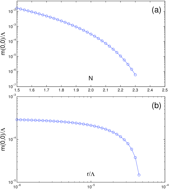
Figure 2: (a) Relationship between dynamical gap $m(0,0)$ and fermion flavor $N$ at nematic QCP, $r=0$; (b) Dependence of $m(0,0)$ on tuning parameter $r$ for $N=2$. Dynamical gap is destroyed once $r$ exceeds certain critical value $r_{c}$.

We now attempt to solve the complicated nonlinear equation (17). Due to the anisotropic nature of nematic fluctuation, the integrations over $\omega$, $k_{1}$, and $k_{2}$ have to be performed separately, which greatly increases the difficulty of numerical computations. For simplicity, here we consider the isotropic limit, $v_{F}=v_{\Delta}$. In this case, the dynamical gap becomes $m(\varepsilon,|\mathbf{p}|)$, and the polarization is simplified to

$$\Pi(\Omega,\mathbf{q}) = \frac{N\lambda^{2}}{16v_{F}^{2}}\frac{2\Omega^{2}+v_{F}^{2}|\mathbf{q}|^{2}}{\sqrt{\Omega^{2}+v_{F}^{2}|\mathbf{q}|^{2}}}.$$ (18)

We first consider the nematic QCP and take $r=0$. In this special case, the pre-factor $\lambda^{2}$ on the right-hand side of equation (17) cancels exactly the factor $\lambda^{2}$ appearing in the polarization function, $\Pi(\epsilon-\omega,\mathbf{p}-\mathbf{k})$, so the gap equation becomes

$$m(\varepsilon,|\mathbf{p}|) = \frac{1}{N}\int\frac{d\omega}{2\pi}\frac{d^{2}\mathbf{k}}{(2\pi)^{2}}\frac{m(\omega,|\mathbf{k}|)}{\omega^{2}+v_{F}^{2}|\mathbf{k}|^{2}+m^{2}(\omega,|\mathbf{k}|)}\frac{16v_{F}^{2}\sqrt{(\epsilon-\omega)^{2}+v_{F}^{2}|\mathbf{p}-\mathbf{k}|^{2}}}{2(\epsilon-\omega)^{2}+v_{F}^{2}|\mathbf{p}-\mathbf{k}|^{2}}.$$ (19)

This gap equation is independent of $\lambda$, and the critical point of dynamical gap generation is therefore solely determined by the flavor $N$. After numerical computations, we find a critical fermion flavor $N_{c}\approx 2.4$ at $r=0$. The nodal qps remain gapless, $m=0$, when $N>N_{c}$, but acquire a nonzero dynamical gap, $m\neq 0$ when $N<N_{c}$. figure 2(a) presents the dependence of the static gap $m(\omega=0,\mathbf{k}=0)$ on flavor $N$. It is clear that the dynamical gap decreases very rapidly as flavor $N$ grows, and vanishes continuously as $N\rightarrow N_{c}$.

It is also interesting to examine how the tuning parameter $r$ of nematic transition affects the dynamical gap generation. Actually, if we move away from the nematic QCP, $r$ becomes finite and the nematic fluctuation is no longer critical. For $r\neq 0$, the coupling parameter $\lambda$ cannot be exactly canceled, but one can absorb it into $r$ by taking $r\rightarrow r/\lambda^{2}$. We find that the dynamical gap is significantly suppressed by growing $r$, and completely destroyed once $r$ exceeds certain critical value $r_{c}$, which is shown in figure 2(b). We therefore conclude that the dynamical gap generation is mediated by the critical fluctuation of nematic order parameter, and exists only in the vicinity of the nematic QCP.

3 Physical implications of dynamical gap

The dynamically generated gap for gapless nodal qps can result in a series of nontrivial physical consequences. In this section, we will discuss the physical implications of the dynamical gap.

Once a nonzero dynamical gap $m$ is generated for the originally gapless nodal qps, there will be an extra term that should be added to the Hamiltonian:

$$H_{\mathrm{m}} = \int\frac{d^{2}\mathbf{k}}{(2\pi)^{2}}\{m(\Psi^{\dagger}_{1\sigma}\tau^{y}\Psi_{1\sigma}+\Psi^{\dagger}_{2\sigma}\tau^{y}\Psi_{2\sigma})\}$$ (20)

$$= \int\frac{d^{2}\mathbf{k}}{(2\pi)^{2}}\left\{im\left[\left(f_{3\downarrow}^{{\dagger}}f_{1\uparrow}^{{\dagger}}+f_{3\downarrow}f_{1\uparrow}\right)+\left(f_{1\downarrow}^{{\dagger}}f_{3\uparrow}^{{\dagger}}+f_{1\downarrow}f_{3\uparrow}\right)+\left(1\leftrightarrow 2,3\leftrightarrow 4\right)\right]\right\}.$$

One can immediately identify that such dynamically generated term corresponds to the formation of singlet Cooper pairs between the gapless nodal qps excited from opposite nodes. We therefore have obtained a secondary, nematic-order driven, $is$-wave superconducting instability on top of the pure $d_{x^{2}-y^{2}}$ superconductivity.

As already pointed out, this dynamical gap is opened only when $r$ is zero or very small, and is rapidly destroyed as $r$ increases, which implies that the secondary $is$-wave superconductivity is achieved only in the close vicinity of nematic QCP. Upon approaching the nematic QCP, there is a zero-temperature phase transition from a pure $d_{x^{2}-y^{2}}$ superconducting state to a fully gapped $d_{x^{2}-y^{2}}+is$ superconducting state. At finite temperature, $T\neq 0$, the critical nematic fluctuation is weakened strongly due to the thermal screening effects, hence the dynamical nodal gap cannot survive at high temperatures. According to these analysis, we now can infer that a small $d_{x^{2}-y^{2}}+is$ superconducting dome emerges around the nematic QCP, which is schematically shown in figure 3. It is interesting to notice that such nematic fluctuation-driven superconducting dome is analogous to that is formed on the border of an antiferromagnetic quantum critical point in the contexts of some heavy fermion compounds [25, 26]. We also notice that the non-perturbative effects of coupling between nodal qps and fluctuating order parameter has been investigated in a physically different context [27].

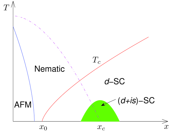
Figure 3: Schematic phase diagram. $x_{c}$ denotes the nematic QCP. The shadowed region around $x_{c}$ represents the emergent fully-gapped $d_{x^{2}-y^{2}}+is$ superconducting dome within a much larger, pure $d_{x^{2}-y^{2}}$ superconducting dome.

We next discuss the effects of nonzero dynamical gap on a number of quantities. First of all, we consider the classical potential between the nodal qps. For simplicity, let us assume a constant gap $m$, which yields a new polarization

$$\Pi(\mathbf{q},\Omega) = \frac{N\lambda^{2}}{2\pi v_{F}v_{\Delta}}\frac{\Omega^{2}+v_{F}^{2}q_{1}^{2}}{Q_{1}}\left[\frac{1}{2}\frac{m}{Q_{1}}+\left(\frac{1}{4}-\frac{m^{2}}{Q_{1}^{2}}\right)\arcsin\left(\frac{Q_{1}}{\sqrt{4m^{2}+Q_{1}^{2}}}\right)\right]$$ (21)

$$+(q_{1}\leftrightarrow q_{2}).$$

In the low energy limit, it takes the simplified form

$$\Pi(\mathbf{q},\Omega)\approx\frac{N\lambda^{2}}{12\pi v_{F}v_{\Delta}m}(2\Omega^{2}+v_{F}^{2}|\mathbf{q}|^{2}).$$ (22)

Using this simplified polarization, it is easy to obtain an effective potential

$$V(\mathbf{R}) \propto \int\frac{d^{2}\mathbf{q}}{(2\pi)^{2}}\frac{e^{i\mathbf{q}\cdot\mathbf{R}}}{\Pi(\mathbf{q})}$$ (23)

$$\propto \frac{6v_{\Delta}}{N\lambda^{2}v_{F}}m\ln(mR)$$

between two massive fermions [28]. This potential grows logarithmically as the distance $R$ is increasing, so the gapped fermions are weakly confined. Such gap-induced fermion confinement is similar to that in a physically analogous theory of QED₃ [28].

When the nodal qps are massless, their velocities are renormalized by the nematic fluctuation and thus become strongly momentum-dependent,

$$v_{F,\Delta}\rightarrow v_{F,\Delta}(k).$$ (24)

The expressions of the renormalized velocities $v_{F,\Delta}(k)$ are quite complicated and therefore not shown here, but can be easily found in Refs. [15, 18]. Both $v_{F}(k)$ and $v_{\Delta}(k)$ vanish as $k\rightarrow 0$. However, $v_{\Delta}(k)$ vanishes much more rapidly than $v_{F}(k)$, leading to the so-called extreme velocity anisotropy [15, 16, 17, 18, 19],

$$\delta(k)=\frac{v_{\Delta}(k)}{v_{F}(k)}\rightarrow 0.$$ (25)

Nevertheless, once a finite fermion gap $m$ is opened, there is no longer strong renormalization of velocities. As shown in figure 4, the velocities $v_{F,\Delta}$ are still $k$-dependent and decrease with decreasing $k$ at high energies, but saturate to finite values once $k$ is smaller than the scale set by $m$. Therefore, the singular velocity renormalization and the extreme anisotropy are both prevented by fermion gap $m$.

The dynamical fermion gap has important impacts on a number of observable quantities. For example, the density of state of nodal qps is linear in energy, $\rho(\omega)\propto|\omega|$, when $m=0$, but becomes $\rho(\omega)\propto|\omega|\theta\left(|\omega|-m\right)$ when $m\neq 0$, which vanishes for $|\omega|<m$. Accordingly, the specific heat of nodal qps is strongly suppressed as $C_{V}(T)\propto m^{4}\exp(-m/T)/T^{2}$ in the low-temperature region of $T\ll m$. Furthermore, the low temperature dc thermal conductivity at finite $m$ is known to have the form [29], $\frac{\kappa}{T}=\frac{k_{B}^{2}}{3}(\frac{v_{F}}{v_{\Delta}}+\frac{v_{\Delta}}{v_{F}})\frac{\Gamma^{2}}{\Gamma^{2}+m^{2}}$, where $\Gamma$ is the impurity scattering rate. In the massless limit, $m=0$, the thermal conductivity is a constant, $\frac{\kappa}{T}=\frac{k_{B}^{2}}{3}(\frac{v_{F}}{v_{\Delta}}+\frac{v_{\Delta}}{v_{F}})$, which is finite and impurity independent [23]. In contrast, once a fermion gap is generated, the thermal conductivity is suppressed by the finite $m$.

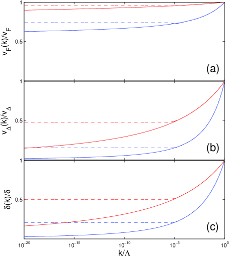
Figure 4: Momentum dependence of fermion velocities $v_{F,\Delta}(k)$ and velocity ratio $\delta(k)=v_{\Delta}(k)/v_{F}(k)$. Here, $v_{F,\Delta}$ and $\delta$ are bare values of the corresponding quantities. Blue solid line: $\delta=1$ and $m=0$; Red Solid line: $\delta=0.1$ and $m=0$; Blue dashed line: $\delta=1$ and $m/v_{F}\Lambda=10^{-6}$; Red dashed line: $\delta=0.1$ and $m/v_{F}\Lambda=10^{-6}$.

Finally, notice that the nematic state is indeed equivalent to a superconducting state with $d_{x^{2}-y^{2}}+s$ gap, which was pointed out in Ref. [21, 22]. Therefore, in the vicinity of a quantum critical point between a pure $d_{x^{2}-y^{2}}$ superconducting state and a $d_{x^{2}-y^{2}}+s$ superconducting state, the singular fluctuation of $s$-wave order parameter can also lead to a fully gapped $d_{x^{2}-y^{2}}+is$ superconducting state, provided that the flavor $N$ of nodal qps is smaller than the corresponding critical value $N_{c}$.

4 Summary and discussions

In summary, we perform non-perturbative analysis within an effective field theory of the strong interaction between the critical nematic fluctuation and nodal qps in the context of d-wave HTSCs. We propose that a dynamical gap may be generated for the originally gapless nodal qps in the vicinity of the nematic QCP. Such gap generation is driven by the critical fluctuation of nematic order parameter and corresponds to an additional $is$-wave Cooper pairing instability. In the vicinity of the nematic QCP, there will be an small emergent $d_{x^{2}-y^{2}}+is$ superconducting dome. We also discuss the physical implications of the dynamically generated gap, and show that such gap leads to weak confinement of nodal qps, saturation of velocity renormalization, and strong suppression of several observable quantities.

According to our results, it turns out that the fermion flavor $N$ is a crucial parameter which determines the low-energy behaviors caused by the nematic order. A critical value $N_{c}$ is found to exist. When $N>N_{c}$, the non-perturbative effects of nematic fluctuation is unimportant, so one can trust the results obtained by perturbative calculations, such as extreme anisotropy [15] and other unusual properties [14, 16, 17, 18, 20, 19]. If $N<N_{c}$, however, the non-perturbative effects become significant, and can drive an additional $is$-wave superconducting pairing between the originally gapless nodal qps.

Our leading-order calculations found that $N_{c}\approx 2.4$, which is larger than the physical flavor $N=2$. It would be interesting to study how $N_{c}$ is quantitatively affected by high order corrections. In principle, it is straightforward to address this issue by coupling the equations of wave function renormalizations $A_{0,1,2}$ and vertex corrections to the gap equation. Unfortunately, solving these coupled equations is a highly challenging task because the integrations over three components of momentum, $\omega,k_{1},k_{2}$, have to be performed separately due to the non-relativistic and spatially anisotropic feature of the present system. It is quite difficult to get reliable numerical solutions. We expect that large scale Monte Carlo simulations would be utilized to investigate this problem and help to determine the precise value of $N_{c}$.

Irrespective of whether our $N_{c}$ is precise or not, a general trend can be deduced from our results: the conventional perturbative $1/N$ expansion should be reliable for large $N$, but it may fail to capture some fundamental features of strongly interacting model for small $N$ and non-perturbative analysis should be utilized instead. In addition, our prediction of a nematic order-induced $d_{x^{2}-y^{2}}+is$ superconducting dome is novel and would shed light on the investigation of nematic order in correlated electron systems.

In our present analysis, we have considered only clean $d$-wave superconductors and ignored the disorder effects. The influence of various quenched disorders on the stability of nematic QCP was investigated in a recent paper [18]. As shown in this paper [18], the strong coupling between critical nematic fluctuation and gapless nodal qps is actually not affected by weak random gauge potential and weak random mass [18]. On the contrary, random chemical potential is able to destroy nematic QCP and thus can fundamentally change the whole picture. However, both these conclusions and the analytical methods used in Ref. [18] are valid only in the particular case that the non-perturbative effects of nematic fluctuation are unimportant and all the nodal qps are strictly gapless. Once the non-perturbative effect becomes strong enough to generate a dynamical fermion gap, the influence of disorders might be quite different. Generically, the dynamical gap generation and disorder scattering can affect each other [30], so they should be investigated self-consistently, as we have done in a physically similar context [30]. Nevertheless, this issue is beyond the scope of the present paper, and would be addressed in the future. In any case, we believe the results presented in this paper are reliable in clean d-wave superconductors and pointed out an interesting new possibility regarding the exotic effects of nematic order.

References

References

- [1] Kivelson S A, Fradkin E and Emery V J 1998 Nature (London) 393 550
- [2] Kivelson S A, Bindloss I P, Fradkin E, Oganesyan V, Tranquada J M, Kapitulnik A and Howald C 2003 Rev. Mod. Phys. 75 1201
- [3] Fradkin E, Kivelson S A, Lawler M J, Eisenstein J P and Mackenzie A P 2010 Annu. Rev. Condens. Matter Phys. 1 153
- [4] Fradkin E 2012 in Modern Theories of Many-Particle Systems in Condensed Matter Physics edited by Cabra D C, Honecker A and Pujol P Lecture Notes in Physics Vol. 843 (Berlin Heidelberg: Springer-Verlag)
- [5] Vojta M 2009 Adv. Phys. 58 699
- [6] Ando Y, Segawa K, Komiya S and Lavrov A N 2002 Phys. Rev. Lett. 88 137005
- [7] Hinkov V, Haug D, Fauqué B, Bourges P, Sidis Y, Ivanov A, Bernhard C, Lin C T and Keimer B 2008 Science 319 597
- [8] Daou R, Chang J, LeBoeuf D, Cyr-Choinière O, Laliberté F, Doiron-Leyraud N, Ramshaw B J, Liang R, Bonn D A, Hardy W N and Taillefer L 2010 Nature (London) 463 519
- [9] Lawler M J, Fujita K, Lee J, Schmidt A R, Kohsaka Y, Kim C K, Eisaki H, Uchida S, Davis J C, Sethna J P and Kim E-A 2010 Nature 466 347
- [10] Chuang T-M, Allan M-P, Lee J, Xie Y, Ni N, Bud’ko S L, Boebinger G S, Canfield P C and Davis J C 2010 Science 327 181
- [11] Okazaki R, Shibauchi T, Shi H J, Haga Y, Matsuda T D, Yamamoto E, Onuki Y, Ikeda H and Matsuda Y 2011 Science 331 439
- [12] Borzi R A, Grigera S A, Farrell J, Perry R S, Lister S J S, Lee S L, Tennant D A, Maeno Y and Mackenzie A P 2007 Science 315 214
- [13] Cooper K B, Lilly M P, Eisenstein J P, Pfeiffer L N and West K W 2002 Phys. Rev. B 65 241313
- [14] Kim E-A, Lawler M J, Oreto P, Sachdev S, Fradkin E and Kivelson S A 2008 Phys. Rev. B 77 184514
- [15] Huh Y and Sachdev S 2008 Phys. Rev. B 78 064512
- [16] Xu C, Qi Y and Sachdev S 2008 Phys. Rev. B 78 134507
- [17] Fritz L and Sachdev S 2009 Phys. Rev. B 80 144503
- [18] Wang J, Liu G-Z and Kleinert H 2011 Phys. Rev. B 83 214503
- [19] Liu G-Z, Wang J-R and Wang J 2012 Phys. Rev. B 85 174525
- [20] Wang J and Liu G-Z 2012 arXiv:1205.6164.
- [21] Vojta M, Zhang Y and Sachdev S 2000 Phys. Rev. B 62 6721
- [22] Vojta M, Zhang Y and Sachdev S 2000 Int. J. Mod. Phys. B 14 3719
- [23] Durst A C and Lee P A 2000 Phys. Rev. B 62 1270
- [24] Sachdev S 2011 Quantum Phase Transitions Chap. 17 (Cambridge University Press)
- [25] Löhneysen H v, Rosch A, Vojta M and Wölfle P 2007 Rev. Mod. Phys. 79 1015
- [26] Stockert O, Kirchner S, Steglich F and Si Q 2012 J. Phys. Soc. Jpn. 81 011001
- [27] Khveshchenko D V and Paaske J 2001 Phys. Rev. Lett. 86 4672
- [28] Maris P 1995 Phys. Rev. D 52 6087
- [29] Gusynin V P and Miransky V A 2004 Eur. Phys. J. 37 363
- [30] Liu G-Z and Wang J-R 2011 New J. Phys. 13 033022