Optimizing MapReduce for Highly Distributed Environments

Abstract

MapReduce, the popular programming paradigm for large-scale data processing, has traditionally been deployed over tightly-coupled clusters where the data is already locally available. The assumption that the data and compute resources are available in a single central location, however, no longer holds for many emerging applications in commercial, scientific and social networking domains, where the data is generated in a geographically distributed manner. Further, the computational resources needed for carrying out the data analysis may be distributed across multiple data centers or community resources such as Grids. In this paper, we develop a modeling framework to capture MapReduce execution in a highly distributed environment comprising distributed data sources and distributed computational resources. This framework is flexible enough to capture several design choices and performance optimizations for MapReduce execution. We propose a model-driven optimization that has two key features: (i) it is end-to-end as opposed to myopic optimizations that may only make locally optimal but globally suboptimal decisions, and (ii) it can control multiple MapReduce phases to achieve low runtime, as opposed to single-phase optimizations that may control only individual phases. Our model results show that our optimization can provide nearly 82% and 64% reduction in execution time over myopic and single-phase optimizations, respectively. We have modified Hadoop to implement our model outputs, and using three different MapReduce applications over an 8-node emulated PlanetLab testbed, we show that our optimized Hadoop execution plan achieves 31-41% reduction in runtime over a vanilla Hadoop execution. Our model-driven optimization also provides several insights into the choice of techniques and execution parameters based on application and platform characteristics.

1 Introduction

1.1 Motivation

The growing need for analysis of large quantities of data generated globally by increasing numbers of users, applications, sensors, and devices has led to wide popularity of the MapReduce [10] model and its open-source Hadoop [14] implementation. MapReduce is widely used today for many data analysis applications, including for example Web indexing, log file analysis, and recommendation mining.

MapReduce has traditionally been deployed over a tightly-coupled cluster or data center, with the assumption that the data is already available at a centralized location, co-located with the computational resources. For many emerging applications and environments, however, data sources are inherently distributed, and the assumption of centralized data and centralized computational resources does not hold. For instance, a number of technology companies as well as traditional businesses such as retail [25] generate data at multiple sites including stores and warehouses situated in diverse locations. Further, large Internet-scale services such as Akamai [23] have highly distributed server deployments spanning thousands of global locations. Each location produces tens of terabytes of data daily, and this data must be aggregated and analyzed. As further examples, many data-intensive scientific applications need to analyze data generated by distributed scientific sensors, instruments, and testbeds, while the data for several social networking applications is generated by millions of users around the world. For such applications, moving data to a central location for analysis can be extremely costly, both in time and money [4].

Besides the data sources being distributed, the computational resources needed for carrying out the data analysis may themselves be distributed. Examples include multiple data centers that may be used by a large Internet company to analyze data local to these data centers, as well as community resources such as Grids used for scientific computation. The ever-growing need for efficient execution of MapReduce computations in highly-distributed environments is the key motivator of our work.

MapReduce efficiency is itself a well-studied problem. Several techniques [30, 2, 9] have been proposed to improve the performance of MapReduce in local cluster environments. It is unclear, however, which of these techniques (if any) are well-suited for executing MapReduce in highly distributed environments. Recent work [7] that explored deploying MapReduce in a highly distributed environment concluded that there is no single architecture or deployment strategy that works well for all possible application, data, network, and system characteristics. Thus, the tradeoffs of deploying and executing MapReduce in a highly distributed environment are not well understood. Further, few guidelines exist on how to efficiently execute a MapReduce application in such an environment. The focus of our work is to provide such guidelines by modeling the characteristics of the application and the distributed environment and devising an optimized “execution plan” that can guide the efficient execution of a MapReduce job.

1.2 The MapReduce framework

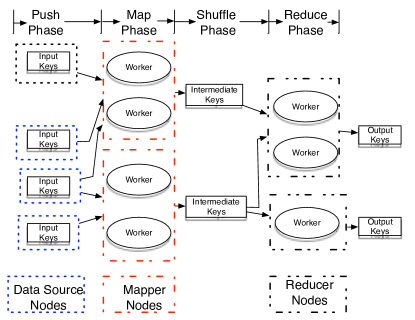
Figure 1: Executing a MapReduce application in a distributed environment. Each node represents a cluster of machines deployed in a data center. In a highly distributed and heterogeneous environment, the nodes have varying amounts of resources distributed across a wide-area network.

The MapReduce programming framework can be used to implement a number of commonly-used applications that take a set of input key/value pairs and produce a set of output key/value pairs [10]. A typical MapReduce application consists of a map function that processes input key/value pairs from the input data to generate a set of intermediate key/value pairs, and a reduce function that merges all intermediate values associated with the same intermediate key to produce the output key/value pairs. We illustrate the execution of a typical MapReduce application in a highly distributed environment in Figure 1. The input data originates at the data source nodes and is distributed to the mapper nodes in the push phase. In the map phase, each mapper node that consists of multiple worker threads running on multiple machines within a cluster performs the map operation on the incoming data and outputs intermediate key/value pairs. In the shuffle phase, the intermediate key/value pairs are partitioned and distributed to the reducer nodes such that all records that correspond to a given intermediate key are sent to the same reducer node. This requirement preserves the semantics of a MapReduce application where all values of a specific intermediate key are required to perform the correct reduction. In the reduce phase, the reducer nodes process the intermediate key/value pairs and produce the final output.

Our notion of efficiency for the execution of a MapReduce job is makespan, defined to be the total time taken for the job to complete. Given a highly distributed platform in the form of multiple machine clusters deployed in a wide-area network and given a MapReduce application, our goal is to optimize the makespan of executing the MapReduce application on the distributed platform.

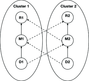
Figure 2: An example of a two-cluster distributed environment, with one data source, one mapper, and one reducer in each cluster. The intra-cluster “local” communication links are solid lines, while the inter-cluster “non-local” communication links are the dotted lines.

1.3 An optimization example

In order to optimize the makespan of MapReduce, we illustrate the criticality of optimizing the data communication and task placement in a distributed environment with a simple example, and show that the best approach depends on the platform and application characteristics.

Consider the example MapReduce platform shown in Figure 2. Assume that the data sources $D1$ and $D2$ have 150$\,\mathrm{GB}$ and 50$\,\mathrm{GB}$ of data, respectively. Let us model a parameter $\alpha$ that represents the ratio of the amount of data output by a mapper to its input; i.e., $\alpha$ is the expansion (or reduction) of the data in the map phase and is specific to the application. We model different situations below.

First, consider a situation where $\alpha=1$ and the network is perfectly homogeneous. That is, all links have the same bandwidth—say 100$\,\mathrm{MBps}$ each—whether they are local or non-local, and the computational resources at each mapper and reducer are homogeneous too; say, each can process data at the rate of 100$\,\mathrm{MBps}$. Clearly, in this case, a uniform data placement, where each data source (resp., mapper) pushes an equal amount of data to each mapper (resp., reducer), produces the minimum makespan.

Now, consider a slight modification to the above scenario. Assume now that the non-local links become much slower and can only transmit at 10$\,\mathrm{MBps}$, while all other parameters remain the same. Now, a uniform data placement no longer produces the best makespan. Since the non-local links are much slower, it makes sense to avoid non-local links when possible. In fact, a plan where each data source pushes all of its data to its own local mapper completes the push phase in $150\,\mathrm{GB}/100\,\mathrm{MBps}=1500$ seconds, while the uniform push would have taken $75\,\mathrm{GB}/10\,\mathrm{MBps}=7500$ seconds. Although the map phase for the uniform placement would be smaller by $50\,\mathrm{GB}/100\,\mathrm{MBps}=500$ seconds, the local push approach makes up for this through a more efficient data push.

Finally, consider the same network parameters above where local links are fast (100$\,\mathrm{MBps}$) and non-local links are slow (10$\,\mathrm{MBps}$). However imagine that $\alpha$ is very large and equals 10, implying that there is 10 times more data in the shuffle phase than in the push phase. The local push no longer performs well, since it does nothing to alleviate the communication bottleneck in the shuffle phase. To avoid non-local communication in the shuffle phase, it makes sense for data source $D2$ to push all of its 50$\,\mathrm{GB}$ of data to mapper $M1$ in the push phase, so that all the reduce can happen within cluster 1 without having to use non-local links in the communication-heavy shuffle phase. This is an example of how an optimization would have to look at all phases in an end-to-end fashion to find a better makespan. In fact, the local push still minimizes the push time from a myopic perspective; i.e., it makes a locally optimal decision which is globally suboptimal in terms of makespan.

The above simple example illustrates the types of considerations in speeding up MapReduce in distributed environments. Our goal in the rest of the paper is to model the distributed environment and the MapReduce application accurately and to evolve techniques that can automatically produce an optimal plan for executing the MapReduce job so as to minimize makespan.

We note that there are two types of optimizations that can be used to speed up a MapReduce computation: dynamic and static. Dynamic optimization works at runtime as the MapReduce computation is being executed. Hadoop and other MapReduce software frameworks implement several dynamic optimizations such as speculative task execution and work stealing. In contrast to dynamic optimizations, static optimizations are performed even before the MapReduce job starts execution, and are hence a complementary form of optimization. Our focus here is on static optimization and we are concerned with producing the optimum data placement and task execution plan for a MapReduce job, taking into account the underlying distributed data sources, network resources, compute resources, and application characteristics.

1.4 Research contributions

Our paper makes the following research contributions:

• We develop a framework for modeling the performance of MapReduce in a highly distributed setting. Our modeling framework is flexible enough to capture a large number of design choices and optimizations. Our work provides a framework for answering “what-if” questions on the relative efficacy of various design alternatives. In particular, our model enables us to compare various architectural choices as well as to provide rules of thumb for efficient deployment based on network and application characteristics. Further, optimizations using our model are efficiently solvable as Mixed Integer Programs (MIP) using powerful solver libraries.

• We modify Hadoop to implement our model outputs and use this modified Hadoop implementation along with network and node measurements from the PlanetLab [8] testbed to validate our model and evaluate our proposed optimization. Our model results show that for a highly distributed compute environment, our end-to-end, multi-phase optimization can provide nearly 82% and 64% reduction in execution time over myopic and the best single-phase optimizations, respectively. Further, using three different applications over an 8-node testbed emulating PlanetLab network characteristics, we show that our statically-enforced optimized Hadoop execution plan achieves 31-41% reduction in runtime over a vanilla Hadoop execution employing its dynamic scheduling techniques.

• Our model-driven optimization provides several insights into the choice of techniques and execution parameters based on application and platform characteristics. For instance, we find that an application’s data expansion factor $\alpha$ can influence the optimal execution plan significantly, both in terms of which phases of execution are impacted more and where pipelining is more helpful. Our results also show that as the network becomes more distributed and heterogeneous, our optimization provides higher benefits (82% for globally distributed sites vs. 37% for a single local cluster over myopic optimization), as it can exploit heterogeneity opportunities better. Further, these benefits are obtained independent of the application characteristics.

2 Models and optimization algorithms

We successively model the distributed platform, the MapReduce application, valid execution plans, and their makespan.

2.1 Modeling the distributed platform and the MapReduce application

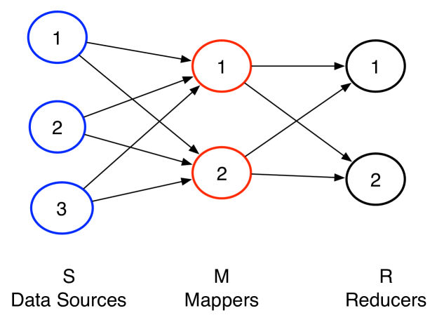
Figure 3: A tripartite graph model for distributed MapReduce with 3 data sources, 2 mappers and 2 reducers.

We model the distributed platform available for executing the MapReduce application as a tripartite graph with a vertex set of $V=S\cup M\cup R$, where $S$ is the set of data sources, $M$ is the set of mappers, and $R$ is the set of reducers. The edge set $E$ of the tripartite graph is the complete set of edges and equals $(S\times M)\cup(M\times R)$ (See Figure 3). Each node corresponds to a cluster of servers that can potentially be used for executing the MapReduce application and the edges represent communication paths between clusters. The capacity of a node $i\in M\cup R$ is denoted by $C_{i}$ (in bits/second), where the capacity captures the computational resources available at that node in the units of bits of incoming data that it can process per second. Note that $C_{i}$ is also application-dependent as different MapReduce applications are likely to require different amounts of computing resources to process the same amount of data. Likewise, the capacity of an edge $(i,j)\in E$ is denoted by $B_{ij}$ that represents the bandwidth (in bits/second) that can be sustained on the communication link that the edge represents.

Rather than model the MapReduce application in detail, we model two key parameters. First, we model the amount of data $D_{i}$ (in bits) that originates at data source $i$, for each $i\in S$. Further, we model an expansion factor $\alpha$ that represents the ratio of the size of the output of a mapper to the size of its input. Note that $\alpha$ can take values less than, greater than, or equal to $1$ depending on whether the output of the map operation is smaller than, larger than, or equal in size to the input. The value of $\alpha$ can be determined by profiling the MapReduce application. Many applications perform extensive aggregation, for example to count the number of occurrences of each word in a set of documents, or to find the $k$ most extreme values in a large set. These applications have $\alpha$ much less than 1. On the other hand, some applications may require intermediate data to be broadcast from one mapper to multiple reducers [24], or to otherwise transform the inputs to produce larger intermediate data, yielding $\alpha>1$.

2.2 Modeling a valid execution plan and its makespan

We define the notion of an execution plan to capture the manner in which data and computation of a MapReduce application are scheduled on a distributed platform. Intuitively, an execution plan determines how the data is distributed from the sources to the mappers and how the intermediate keys produced by the mappers are distributed across the reducers. Thus, the execution plan determines which nodes and which communication links are used and to what degree, and is therefore a major determinant of how long the MapReduce application takes to complete.

An execution plan of the MapReduce application on the distributed platform is represented by variables $x_{ij}$, for $(i,j)\in E$, that represent the fraction of the outgoing data from node $i$ that is sent to node $j$. From a high level, an execution plan can be implemented by extending the MapReduce software framework as follows. Note that existing MapReduce frameworks such as Hadoop partition the input key space at the data sources and assign each partition to a mapper. Likewise, implementations partition the intermediate key space output by the mappers, and assign each partition to a reducer. As we mention later, this partitioning is usually achieved by a simple uniform hash function that divides the key space evenly into the required number of buckets. Generalizing this concept, we can allow each data source and mapper to use its own hash function to partition the input and intermediate key spaces respectively, even perhaps in a non-uniform fashion. This enables the implementation of any execution plan $x_{ij}$, for $(i,j)\in E$, by simply providing a hash function $h_{i}$ to each node $i\in S$ (resp. $i\in M$) such that a fraction $x_{ij}$ of the input keys (resp., intermediate keys) are sent to mapper $j$ (resp., reducer $j$). We describe such an approach more concretely in Section 3.1.

Valid execution plans. We now mathematically express sufficient conditions for an execution plan to be valid and implementable in a MapReduce software framework while obeying the MapReduce application semantics.

$$\forall(i,j)\in E:0\leq x_{ij}\leq 1$$ (1)

$$\forall i\in V:\sum_{(i,j)\in E}x_{ij}=1$$ (2)

Equations 1 and 2 simply express that for each $i$, the $x_{ij}$’s are fractions that sum to $1$.

The semantics of a MapReduce application requires that each intermediate key be mapped to a single reducer. This is typically achieved by partitioning the intermediate key space among all the reducers and ensuring that each reducer gets all the keys in its assigned key space. This semantics can be implemented by ensuring that all mappers use the same hash function to map intermediate keys to reducers. Define variable $y_{k}$, $k\in R$, to be the fraction of the key space mapped to reducer $k$. We enforce the one-reducer-per-key requirement with the following constraint.

$$\forall j\in M,k\in R:x_{jk}=y_{k}.$$ (3)

We define an execution plan to be valid if Equations 1, 2, and 3 hold.

Modeling the consecutive execution of phases. The push, map, shuffle, and reduce phases are executed in sequence. Between each pair of consecutive phases, there are three possible assumptions that we can make. The simplest assumption is that a global barrier exists between the two consecutive phases. That is, all nodes must complete any given phase before any node can proceed to the next phase. While the global barrier satisfies data dependencies across the different phases, it has no concurrency in terms of the execution of the phases. Alternately, one can assume that a local barrier exists between the two consecutive phases. With a local barrier, each node can start the next phase as soon as it receives all its inputs from the previous phase without waiting for other nodes to complete the previous phase. For instance, with a local barrier, a node can start the map or reduce phase as long as it has all of its input data, and a node can start the push and shuffle phases as long as it has all the data that it needs to disseminate. In particular, a node need not wait for other nodes to complete the current phase before proceeding to the next phase. This allows a greater degree of concurrency between the execution of the different phases, allowing the makespan to be reduced. The third option of pipelining provides the greatest amount of concurrency and has the potential for the lowest makespan among the three options. Pipelining allows a node to start the map or reduce phase as long as the first piece of its input data is available for processing; i.e., the node need not wait for all of its inputs to be present but rather it can start as soon as it receives the first piece. Likewise, a node can start the push and shuffle phases as soon as it receives the first piece of the data that needs to be disseminated. It is easy to see that pipelining allows for even more concurrency than local barriers.

Which of these three options is allowable for each pair of consecutive phases depends on application semantics and how the application itself is implemented. For instance, for a specific application, a reducer may be able to proceed independently of other reducers, but may need to wait until it receives all of its intermediate data before it can start execution. In this case, a local barrier is allowable, but pipelining is not. Or, perhaps the application is such that incremental processing is possible in each phase without receiving all of the input data, which is amenable to pipelining. We now show how to model each of these three possibilities starting with the simplest case where all barriers are global.

Makespan of a valid execution plan with global barriers. Given a valid execution plan for a MapReduce application, we now model the total time to completion, i.e., its makespan. To model the makespan, we successively model the time to completion of each of the four phases assuming that a global barrier exists after each phase. We assume that the data is available at all the data sources at time zero when the push phase begins. For each mapper $j\in M$, the time for the push phase to end is denoted by ${\mathrm{push\_end}}_{j}$ that equals the time when all its data is received; i.e.,

$$\forall j\in M:{\mathrm{push\_end}}_{j}=\max_{i\in S}\frac{D_{i}x_{ij}}{B_{ij}}.$$ (4)

Since we assume a global barrier after the push phase, all mappers must receive their data before the push phase ends and the map phase begins. Thus, the time when the map phase starts denoted by ${\mathrm{map\_start}}$ obeys the following equation.

$${\mathrm{map\_start}}=\max_{j\in M}{\mathrm{push\_end}}_{j}$$ (5)

The computation at each mapper takes time proportional to the data pushed to that mapper. Thus, the time ${\mathrm{map\_end}}_{j}$ for mapper $j\in M$ to complete its computation obeys the following.

$$\forall j\in M:{\mathrm{map\_end}}_{j}={\mathrm{map\_start}}+\frac{\sum_{i\in S}D_{i}x_{ij}}{C_{j}}$$ (6)

As a result of the global barrier, the shuffle phase begins when all mappers have finished their respective computations. Thus, the time ${\mathrm{shuffle\_start}}$ when the shuffle phase starts obeys the following.

$${\mathrm{shuffle\_start}}=\max_{j\in M}{\mathrm{map\_end}}_{j}$$ (7)

The shuffle time for each reducer is governed by the slowest shuffle link into that reducer. Thus the time when shuffle ends at reducer $k\in R$ denoted by ${\mathrm{shuffle\_end}}_{k}$ obeys the following.

$$\forall k\in R:{\mathrm{shuffle\_end}}_{k}=$$

$${\mathrm{shuffle\_start}}+\max_{j\in M}\frac{\alpha\sum_{i\in S}D_{i}x_{ij}x_{jk}}{B_{jk}}$$ (8)

Following the global barrier assumption, the reduce phase computation begins only after all reducers have received all of their data. Let ${\mathrm{reduce\_start}}$ be the time when the reduce phase starts. Then

$${\mathrm{reduce\_start}}=\max_{k\in R}{\mathrm{shuffle\_end}}_{k}.$$ (9)

Reduce computation at a given node takes time proportional to the amount of data shuffled to that node. Thus, the time when reduce ends at node $k$ denoted by ${\mathrm{reduce\_end}}_{k}$ obeys the following.

$$\forall k\in R:{\mathrm{reduce\_end}}_{k}=$$

$${\mathrm{reduce\_start}}+\frac{\alpha\sum_{i\in S}\sum_{j\in M}D_{i}x_{ij}x_{jk}}{C_{k}}$$ (10)

Finally, it is clear that the makespan equals the time at which the last reducer finishes. Thus

$$\mathrm{Makespan}=\max_{k\in R}{\mathrm{reduce\_end}}_{k}.$$ (11)

Modeling local barriers and pipelining. We now show how to modify the above constraints to model local barriers and pipelining. First, we replace the constraints governing the start time for the last three phases as expressed in Equations 5, 7 and 9 with the following new constraints. These new constraints capture the fact that a node can start its next phase without waiting for all nodes to complete the previous phase.

$$\begin{split}\forall j\in M:{\mathrm{map\_start}}_{j}&={\mathrm{push\_end}}_{j}\\ \forall j\in M:{\mathrm{shuffle\_start}}_{j}&={\mathrm{map\_end}}_{j}\\ \forall k\in R:{\mathrm{reduce\_start}}_{k}&={\mathrm{shuffle\_end}}_{k}\end{split}$$

Now we can generalize the definitions for the ending times of these stages by first defining a combination operator $\oplus$ for each optimization as follows:

$$a\oplus b=\begin{cases}a+b,&\text{if local barrier}\\ \max(a,b),&\text{if pipelined}\end{cases}$$

Then, we replace the definition for the ending time of the map phase in Equation 6 with the following new constraint.

$$\forall j\in M:{\mathrm{map\_end}}_{j}={\mathrm{map\_start}}_{j}\oplus\frac{\sum_{i\in S}D_{i}x_{ij}}{C_{j}}$$ (12)

Intuitively, the above constraint specifies that the runtime for the map phase on a node depends on the start-time of the map phase on that node and the time for map computation on all of the data pushed to that node. For the local barrier case, this equals the sum of the two times (corresponding to the time to push the data and then compute on the data in sequence). On the other hand, for the pipelining case, this equals the maximum of the two times, since the map phase at a node cannot end until all of its data has arrived and all of its computation has finished, and the slower of these two operations will dictate the completion time. Note that we are assuming that the data push and map computation are completely overlapped. This assumption is valid if the total quantity of data is much larger than individual record size, which is the case for many typical MapReduce applications.

Based on similar intuition, the constraint for the shuffle stage in Equation 8 is replaced with

$$\forall k\in R:{\mathrm{shuffle\_end}}_{k}=$$

$$\max_{j\in M}\left\{{\mathrm{shuffle\_start}}_{j}\oplus\frac{\alpha\sum_{i\in S}D_{i}x_{ij}x_{jk}}{B_{jk}}\right\}$$ (13)

Finally, the constraint for the end of the reduce stage in Equation 10 is similarly replaced with

$$\forall k\in R:{\mathrm{reduce\_end}}_{k}=$$

$${\mathrm{reduce\_start}}_{k}\oplus\frac{\alpha\sum_{i\in S}\sum_{j\in M}D_{i}x_{ij}x_{jk}}{C_{k}}$$ (14)

2.3 Our optimization algorithm

We formulate the problem of finding the execution plan that minimizes the makespan as an optimization problem. Viewing Equations 1 to 11 as constraints, we need to minimize a profit function that equals the variable $\mathrm{Makespan}$. (Note that if the barriers are not global, the appropriate substitutions of the constraints need to be made.) To perform this optimization efficiently, we rewrite the constraints in linear form to obtain a Mixed Integer Program (MIP). Writing it as MIP opens up the possibility of using powerful off-the-shelf solvers such as the Gurobi version 5.0.0 that we use to derive our results.

There are two types of nonlinearities that occur in our constraints, and these need to be converted to linear form. The first type is the existence of the max operator in Equations 4, 5, 7, 8, 9, and 11. Here we use a standard technique of converting an expression of the form $\max_{i}z_{i}=Z$ into an equivalent set of linear constraints $\forall i:z_{i}\leq Z$, where $Z$ is minimized as a part of the overall optimization.

The second type of non-linearity arises from the quadratic terms in Equations 8 and 10. We remove this type of nonlinearity with a two step process. First, we express the product terms of the form $yz$ that involve two different variables in separable form. Specifically, we introduce two new variables $w=\frac{1}{2}\left(y+z\right)$ and $w^{\prime}=\frac{1}{2}\left(y-z\right)$. This allows us to replace each occurrence of $yz$ with $w^{2}-w^{\prime 2}$, which is in separable form since it does not involve a product of two different variables. Next, we approximate the quadratic terms $w^{2}$ and $-w^{\prime 2}$ with a piecewise linear approximation of the respective function. The more piecewise segments we use the more accuracy we achieve, but this requires a larger number of choice variables resulting in a longer time to solve. As a compromise, we choose about 10 evenly spaced points on the curve leading to an approximation with about $9$ line segments resulting in a worst-case deviation of $4.15\%$ between the piece-wise linear approximation and the actual function. Since $w^{2}$ is a convex function, its piece-wise linear approximation can be expressed using linear constraints with no integral variables. However, since $-w^{2}$ is not a convex function, its piecewise linear approximation requires us to utilize new binary integral variables to choose the appropriate line segment, resulting in a MIP (Mixed Integer Program) instead of an LP (Linear Program). For a more detailed treatment of the techniques that we have used to remove the two types of nonlinearities, the reader is referred to [29].

3 Model implementation and validation

In this section, we discuss how our model outputs could be instantiated in a real MapReduce framework using Hadoop as a representative MapReduce implementation. We have modified Hadoop in order to understand the accuracy of our model outputs as well as to evaluate the benefits of our optimization. Next, we discuss the implementation details of our changes made to Hadoop, followed by validation results for our model based on this implementation.

3.1 Implementing an execution plan in Hadoop

Recall from Section 2 that in our model, a valid MapReduce execution plan is defined as a set of data fractions {$x_{ij}\}$ over all links $(i,j)$ in the MapReduce cluster, where these {$x_{ij}\}$ values satisfy Equations 1, 2, and 3. To enable a valid execution plan to be instantiated in Hadoop, we make three primary modifications to Hadoop: (i) enforcing a tight coupling between data placement and task execution, so that the work carried out on a node strictly depends on the fraction of the data it receives as part of the execution plan; (ii) controlling the push-phase data placement to implement the fraction of data to be sent between each source-mapper pair; and (iii) controlling the shuffle-phase data placement to send the fraction of data between each mapper-reducer pair as per the execution plan. We apply these changes to Hadoop version 1.0.1. Here we discuss each of these changes in detail. In addition, we also discuss how we achieve different barrier configurations (global, local and pipelining) as part of the Hadoop framework.

3.1.1 Coupling data placement and task execution

Our model assumes that the data placement in the push and shuffle phases uniquely determines the task execution in the map and reduce phases respectively. In the map phase, Hadoop attempts to satisfy this assumption using the so-called “locality optimization” [10], whereby a map task is scheduled on a mapper node that already hosts the data for that task. However, this optimization is not strictly enforced in Hadoop. For example, if a mapper node (a TaskTracker in Hadoop parlance) has already completed map tasks for all of the input data that it hosts, it may be assigned map tasks that read inputs from remote nodes. In order to isolate the effects of our optimized plans from such dynamic mechanisms, we add a configuration option (which we call LocalOnly for brevity) to Hadoop to disable assignment of remote tasks. This involves simple modifications to the JobInProgress class, which is responsible for maintaining information about the map and reduce tasks associated with a running job, and for responding to the scheduler’s request for new map and reduce tasks. The existing implementation already supports the data-locality optimization. Specifically, each map task in Hadoop reads its input from an InputSplit, which exposes a getLocations method to the scheduler. This method reports the host(s) on which the task can be considered local; for an InputSplit backed by a file block in the Hadoop Distributed File System (HDFS) for example, getLocations would return the locations of the replicas of that block. Additionally Hadoop allows users to specify the topology of the network. Hadoop uses these two mechanisms to estimate the distance between a TaskTracker and an InputSplit. Our implementation simply checks the status of the LocalOnly configuration parameter, and if it is set, forces the JobInProgress to return to the scheduler only those tasks that are completely local to the requesting TaskTracker.

For reduce tasks, on the other hand, there is no data-locality optimization, as shuffle communication follows an all-to-all pattern in the general case due to the one-reducer-per-key requirement. We couple the intermediate data placement to reduce task execution by establishing a mapping between TaskTrackers and reduce tasks. For ease of implementation, we encode this mapping using Hadoop’s Configuration API, recording which reduce partitions each TaskTracker is allowed to run. Then when the scheduler requests a new reduce task, JobInProgress returns only tasks in this set. If no mapping is specified for a TaskTracker, then reduce task assignment behaves as it does in the default Hadoop.

An additional case where Hadoop might break our assumption occurs when it launches speculative (i.e., backup) tasks. Hadoop already provides a configuration option to disable such speculative tasks, and we employ this control directly.

3.1.2 Controlling data placement in the push phase

Now that we have established the tight coupling between data placement and task execution, we need a way to control the data placement according to the $x_{ij}$ values specified by the execution plan. For map tasks, we achieve this by implementing a custom InputFormat and a corresponding custom InputSplit. The getLocations method behaves as mentioned earlier, by returning the host name for the TaskTracker on which that task should run. The InputSplit is also responsible for providing its map task with a RecordReader for reading inputs. Our InputSplit encodes a list of data sources along with the amount of data to read from each, and it builds a RecordReader that reads from each of these data sources concurrently over TCP sockets. These sockets feed a producer-consumer queue, and the map tasks can read from this queue as a single stream. For ease of implementation, our RecordReader connects to our own simple data source server using TCP sockets.

The traditional FileInputFormat constructs InputSplits that each closely follow HDFS block boundaries, requiring no user control. Our InputFormat, on the other hand, reads a user-provided push plan (as produced by our optimization), and builds a set of InputSplits that achieve the planned push distribution. As an example, if the plan calls for a mapper $M_{1}$ to read 3/4 of its data from data source $S_{1}$ and 1/4 from data source $S_{2}$, then the InputSplits destined for $M_{1}$ will each read 3/4 of their data from $S_{1}$ and 1/4 of their data from $S_{2}$. The size of each individual InputSplit is limited by a user-specified parameter; in our experiments we limit the size to 64MB, the same size we use for HDFS file blocks.

3.1.3 Controlling data placement in the reduce phase

To control the intermediate data placement for reduce tasks, we implement a custom Partitioner class that first partitions intermediate keys into buckets in exactly the same way that a typical Partitioner does (the default simply uses a hash function). We set the number of buckets significantly larger than the number of reduce tasks, then assign an appropriate number of these small buckets to each reduce task. For example, if we have two reducers $R_{1}$ and $R_{2}$, and the plan calls for $R_{1}$ to reduce 2/3 of the intermediate keys, then we assign 2/3 of these buckets to the partition for $R_{1}$, and 1/3 of the buckets to the partition for $R_{2}$. This is possible because, as we discussed earlier, we establish a unique mapping between partition numbers and TaskTrackers. We implement a convenience method to read a plan from a file, and use the Configuration API to configure the Partitioner as well as the partition-to-TaskTracker mapping appropriately.

3.1.4 Instantiating barrier configurations

Our model also allows us to instantiate different barrier configurations (global, local and pipelining) at each phase boundary as part of the MapReduce job execution. We instantiate a subset of all possible barrier configurations in Hadoop: Hadoop supports some of these barrier configurations by default, while we do not consider some of the others that are either hard to implement within the Hadoop framework, or are not immediately interesting. We achieve the following barrier configurations:

• Push/map barriers: To achieve a global barrier at the push/map phase boundary, we run a separate map-only job to enact the push, which uses the custom InputFormat to read directly from the data sources, and writes directly to HDFS. Then we run the main job, which uses a regular FileInputFormat to read directly from HDFS as a typical Hadoop MapReduce job would do. This is the same way the DistCP tool from the Hadoop distribution copies files from one distributed file system to another. Pipelining is achieved by using the custom InputFormat in the main job itself to read directly from the data sources to the mappers. We have not instantiated a local barrier at this phase boundary.

• Map/shuffle barriers: For global barriers, we set the Hadoop configuration parameter
  mapred.reduce.slowstart.completed.maps to 1. This parameter specifies the fraction of map tasks that must complete before any reduce tasks are scheduled, and is often used in shared clusters in order to keep reduce tasks from occupying scarce reduce slots while they are merely waiting for input data. By setting it to 1, we require that all mappers finish before any reducers start. Since the shuffle is actually carried out by reducers pulling their data, if no reducers start until the whole map phase finishes, then there is also no shuffle until the map phase finishes; i.e., map and shuffle phases are separated by a global barrier. Coarse-grained pipelining is essentially the default behavior of Hadoop as long as there are enough reduce slots to schedule all reduce tasks immediately. MapReduce Online [9] implements finer-grained pipelining between these phases, but we consider only Hadoop’s coarse-grained pipelining here. We have not instantiated a local barrier at this phase boundary.

• Shuffle/reduce barriers: Here, local barrier is the default configuration of Hadoop, as a reducer can start as soon as it has finished receiving all of its input data without waiting for other reducers to finish the shuffle phase. Note that implementing pipelining at this boundary is difficult in general: the MapReduce programming model requires that each invocation of the reduce function be provided an intermediate key and all intermediate values for that key. Relaxing the barrier at this phase therefore requires changes at the application level, as Verma et al. [28] describe in detail. We do not implement the global barrier at this phase boundary.

3.2 Model estimation and validation

In this section, we show how the various parameters of our model can be estimated from actual measurements. Further, we validate our model by correlating the model predictions for makespan of different execution plans with the actual measured makespan achieved by our modified Hadoop implementation executing the corresponding plans.

We use PlanetLab [8] for our measurements, since it is a globally distributed testbed and is representative of the highly distributed environment that we are considering in this paper. We measure bandwidth and compute capacities for a set of PlanetLab nodes, and estimate the model parameters for our distributed experimental platform as follows. For each $(i,j)\in E$, bandwidth $B_{ij}$ is estimated by transferring data over that link and measuring the achieved bandwidth. For stable estimates, we used downloads of size at least 64$\,\mathrm{MB}$ or a transfer time of at least 60 seconds, whichever occurs first. For each compute node $i$, we estimate its compute rate $C_{i}$ by measuring the runtime of a simple computation over a list within a Python program, yielding a rate of computation in megabytes per second. This value is not directly useful on its own, but we use it to estimate the relative speeds of different nodes which may be used as part of a distributed MapReduce cluster.

We base these measurements on a set of eight physical PlanetLab nodes distributed across eight sites, including four in the United States, two in Europe, and two in Asia. The unscaled $C_{i}$ values on these nodes range from as low as 9$\,\mathrm{MBps}$ to as high as about 90$\,\mathrm{MBps}$. Table 1 shows the intra-continental and inter-continental link bandwidths for these nodes and highlights the heterogeneity that characterizes such a highly distributed network.

Table 1: Measured bandwidth ($\,\mathrm{KBps}$) of the slowest/fastest links between clusters in each continent.

	US	EU	Asia
US	216 / 9405	110 / 2267	61 / 3305
EU	794 / 2734	4475 / 11053	1502 / 1593
Asia	401 / 3610	290 / 1071	23762 / 23875

To study the predictive power of this model for a range of the application parameter $\alpha$, we implement a synthetic Hadoop MapReduce job that allows direct control over this parameter. Mappers in this job read a key-value pair and emit that same key-value pair an appropriate number of times to achieve the user-specified $\alpha$ value. For example, if $\alpha=0.5$, then this synthetic mapper would directly emit only every other input key-value pair; with $\alpha=2$, it would emit every input key-value pair twice. This job uses an identity reducer. This synthetic application also allows us to emulate computation heterogeneity by carrying out a different amount of computation on each node based on a user-provided parameter.

Using this synthetic job, we can study the predictive power of our model by correlating model predictions and actual measured makespan using the following approach. Given the scaled $C_{i}$ values along with the bandwidth measurements from PlanetLab, we can derive the model’s prediction for makespan by using the model equations (Equations 1 to 11, with substitutions as needed for local barriers or pipelining). We then run a MapReduce job using our prototype implementation in Hadoop. We run this MapReduce job on a local cluster of eight nodes, where each node has two dual-core 2800$\,\mathrm{MHz}$ AMD Opteron 2200 Processors, 4$\,\mathrm{GB}$ RAM, a 250$\,\mathrm{GB}$ disk, and Linux kernel version 2.6.32. The nodes are connected via Gigabit Ethernet and we use tc to emulate the network bandwidths measured on PlanetLab. We use an emulated local testbed to achieve stable and repeatable experiments, as well as due to the daily bandwidth limits and severe memory constraints on PlanetLab, which prevent such data-intensive experiments. Overall, we emulate the full heterogeneity of the PlanetLab environment by using tc to emulate network heterogeneity and our synthetic MapReduce job to emulate computation heterogeneity as well as the parameter $\alpha$.

For our validation, we consider $\alpha$ values of 0.1, 1, and 2. We consider two levels of network heterogeneity: the network conditions measured from PlanetLab as well as no emulation (raw LAN bandwidths). We also consider two levels of computation heterogeneity: those measured from PlanetLab, as well as no emulation. We consider four barrier configurations: G-P-L, P-P-L, P-G-L, and G-G-L, where G, L, and P correspond to global barrier, local barrier and pipelining respectively, and each barrier sequence (e.g., G-P-L) corresponds to the sequence of barriers enacted at push/map, map/shuffle, and shuffle/reduce phase boundaries respectively. We include two types of execution plans: a uniform plan that distributes the input and intermediate data uniformly among the mappers and reducers respectively, as well as an optimized plan generated by our optimization algorithm. All of our plans use 256$\,\mathrm{MB}$ of input data from each of the eight data sources. We use two mappers and one reducer on each of eight compute nodes. Actual makespan varies from 175 seconds to 2849 seconds.

Figure 4: Measured makespan from the Hadoop MapReduce implementation on the local emulated testbed correlates strongly with the model-predicted makespan.

The results of the validation are shown in Figure 4. This figure shows a strong correlation ($R^{2}$ value of 0.9412) between predicted makespan and measured makespan. In addition, the linear fit to the data points has a slope of 1.1464, which shows there is also a strong correspondence between the absolute values of the predicted and measured makespans.

4 Benefits of optimized execution

We provide an intuitive understanding of the optimization algorithm proposed in Section 2.3 and evaluate the benefit of the execution plans that it produces. The two primary aspects that our optimization controls are how much data is sent over which links in each of the push and shuffle phases. Since task scheduling is tightly coupled to data placement, once the push and shuffle phases are specified the entire execution plan is determined.

Our proposed optimization has two key properties. First, it minimizes the end-to-end makespan of the whole MapReduce job, which includes the time from the initial data push to the final reducer execution. Thus, its decisions may be suboptimal for individual phases, but will be optimal for the overall execution of the MapReduce job. Second, our optimization is multi-phase in that it controls the data dissemination across both the push and shuffle phases; i.e., it outputs the best way to perform both the push and shuffle phases so as to minimize makespan. To understand the benefits of our end-to-end multi-phase optimization relative to other schemes, we answer the following questions.

• How beneficial is it to optimize end-to-end makespan as opposed to myopically minimizing the time for a single phase? (Section 4.2)

• How beneficial is it for our optimization to control multiple phases—i.e., both the push and shuffle phases—as opposed to just a single phase? (Section 4.3)

• How much better are optimal execution plans compared with using uniform data placement with no explicit optimization? (Sections 4.2 and 4.3)

• What is the impact on optimized makespan of relaxing the barriers between phases? (Section 4.4)

• What is the impact of the distributed network environment on the optimized execution plan? (Section 4.5)

• How does our optimized execution plan compare to Hadoop? (Section 4.6)

4.1 Experimental setup

To evaluate our optimization schemes, we use PlanetLab measurements to create the different distributed network environments that we use in our experiments. Our network environments vary from a single data center that is relatively homogeneous, to a diverse environment comprising eight globally distributed data centers. To realistically model these environments, we use actual measurements of the compute speed and link bandwidths from PlanetLab nodes distributed around the world, including four in the US, two in Europe, and two in Japan with compute rates and interconnection bandwidths as described in Section 3.2. Using these measurements, we generate the following specific network environments:

• Local data center: This setup consists of one local cluster with eight nodes of each type (source, mapper, reducer), and corresponds to the traditional local MapReduce execution scenario. This cluster is based purely on nodes in the US, specifically at tamu.edu.

• Intra-continental data centers: This setup consists of two data centers located within a continent—all nodes are in the US at tamu.edu and ucsb.edu. This setup corresponds to a more distributed topology than the local cluster scenario.

• Globally distributed data centers: In this setup, nodes span the entire globe (California, Texas, Germany, Japan), introducing much greater heterogeneity and wide-area network bandwidths and latencies. We considered two different global environments: one with four data centers (at ucsb.edu in California, tamu.edu in Texas, tkn.tu-berlin.de in Germany, and pnl.nitech.ac.jp in Japan), and another with eight data centers (same as earlier plus hpl.hp.com in California, uiuc.edu in Illinois, essex.ac.uk in the UK, and wide.ad.jp in Japan). This allows us to compare the impact of scaling up the number of locations.

For each of the above setups, the total number of nodes is held constant at eight. In some cases, where we did not have sufficiently many nodes to meet this requirement (e.g., for the local data center setup), we added replica nodes to the setup with the measured node/link characteristics of the corresponding real nodes. In addition, we held the number of data sources fixed, allocating these data sources to clusters in the same proportion as mappers and reducers. The total amount of input data per data source was held constant throughout.

The globally distributed environment with eight data centers that is described above is most appropriate for studying the general properties of our optimization, as it closely resembles the highly-distributed settings that we focus on in our work. Consequently, we use this environment in all our experiments, except in Section 4.5 where we study the impact of distribution of network resources on our optimization. Therefore, in that section, we use all of the above environments, from the least distributed single data center to the most distributed eight data center environment.

4.2 End-to-End versus myopic

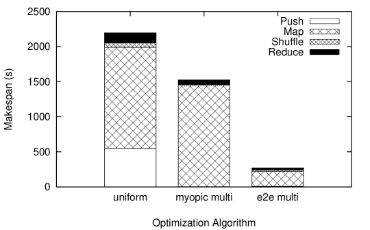
(a) $\alpha$=0.1

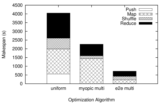
(b) $\alpha$=1

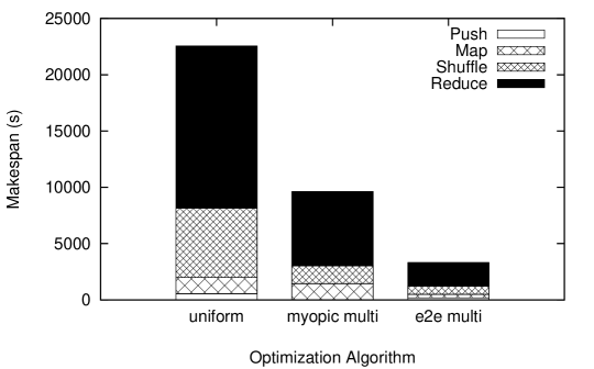
(c) $\alpha$=10

Figure 5: Our proposed end-to-end multi-phase optimization (e2e multi) outperforms the uniform scheme by a large margin (82-87%), while myopic multi-phase optimization (myopic multi) outperforms the uniform scheme by a smaller but still significant margin (30-57%). Our end-to-end multi-phase scheme outperforms myopic multi-phase by a margin of 65-82%, demonstrating the value of end-to-end optimization.

The distinction between end-to-end and myopic optimization is the objective function that is being minimized. With end-to-end, the objective function is the overall makespan of the MapReduce job, whereas a myopic optimizer uses the time for single data dissemination phase (push or shuffle) as its objective function. Myopic optimization is a localized optimization, e.g., pushing data from data sources to mappers in a manner that minimizes the data push time. Such local optimization might result in suboptimal global execution times by creating bottlenecks in other phases of execution. Note that myopic optimization can be applied to both push and shuffle phases in succession. That is, the push phase is first optimized to minimize push time and then the shuffle phase is optimized to minimize shuffle time assuming that the input data has been pushed to mappers according to the first optimization.

The myopic optimizations described above can be achieved by modifying our formulation in Section 2 as follows. Instead of minimizing makespan, we replace Equation 11 with alternate objective functions. For optimizing the push time we use: minimize $\max_{j\in M}{{\mathrm{push\_end}}_{j}}$, and to optimize the shuffle time we use: minimize $\max_{k\in R}{{\mathrm{shuffle\_end}}_{k}}$, where $M$ and $R$ are the sets of mapper and reducer nodes respectively. (Note that computing a myopic multi-phase plan requires solving several optimizations in sequence.)

As a comparative baseline, we would also like to evaluate the makespan produced by the uniform schedule that involves no optimization at all. In a uniform schedule, we distribute the input data across the mappers uniformly, and also distribute the intermediate data across the reducers uniformly. This could be expressed in our model using the following additional constraints:

$$\mathrm{Uniform\ Push:} \forall i\in S,j\in M:x_{ij}=\frac{1}{|M|}$$ (15)

$$\mathrm{Uniform\ Shuffle:} \forall j\in M,k\in R:x_{jk}=\frac{1}{|R|}$$ (16)

The above constraints implicitly assume that the nodes and communication links are homogeneous, so that the sources uniformly distribute their data to the mappers, and the mappers uniformly distribute their data to the reducers.

In Figure 5, we show the makespan achieved in three different cases: (i) for a uniform data placement; (ii) for a myopic, multi-phase optimization, where the push and shuffle phases are optimized myopically in succession; and (iii) for our end-to-end, multi-phase optimization that minimizes the total job makespan. Note that since both (ii) and (iii) are multi-phase, the primary difference between them is that one is myopic and the other is end-to-end, helping us determine the relative merits of end-to-end versus myopic approaches. We evaluated these three schemes for different assumptions for $\alpha$. We see that, for each $\alpha$, the myopic optimization reduces the makespan over the uniform data placement approach (by 30, 44, and 57% for $\alpha$ = 0.1, 1, and 10 respectively), but is significantly outperformed by the end-to-end optimization (which reduces makespan by 87, 82, and 85%). This is because, although the myopic approach makes locally optimal decisions at each phase, these decisions may be globally suboptimal, while our end-to-end optimization makes globally optimal decisions. As an example, for $\alpha$=0.1, while both the myopic and end-to-end approaches dramatically reduce the push time over the uniform approach (by 99.4 and 98.5% respectively), the end-to-end approach is also able to reduce the map time substantially (by 85%) whereas the myopic approach makes no improvement to the map time. A similar trend is evident for $\alpha$=10, where the end-to-end approach is able to lower the reduce time significantly (by 68%) over the myopic approach. These results show the benefit of an end-to-end, globally optimal approach over a myopic, locally optimal but globally suboptimal approach.

4.3 Single-phase versus multi-phase

The distinction between single-phase and multi-phase is which phase (push, shuffle, or both) is controlled by the optimization, and is orthogonal to the end-to-end versus myopic distinction. A single-phase optimization controls the data distribution of one phase—e.g., the push phase—alone, while using a uniform data distribution for the other communication phase. A single-phase optimization is myopic if it minimizes the time for that phase alone. However, it could also be end-to-end if it optimizes the phase so as to achieve the minimum overall makespan. A single-phase optimization may be achieved in our model by using one of the uniform push or shuffle constraints (Equation 15 or 16) to constrain the data placement for one of the phases, while allowing the other phase to be optimized.

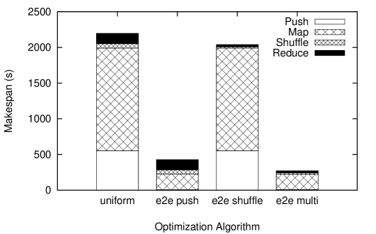
(a) $\alpha$=0.1

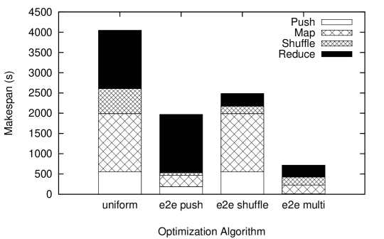
(b) $\alpha$=1

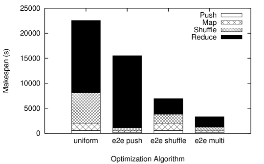
(c) $\alpha$=10

Figure 6: Our end-to-end multi-phase optimization (e2e multi) performs better than end-to-end push (e2e push) and end-to-end shuffle (e2e shuffle), demonstrating the value of multi-phase optimization. In addition, all forms of optimization perform better than uniform.

In Figure 6, we compare (i) a uniform data placement, (ii) an end-to-end single-phase push optimization that assumes a uniform shuffle, (iii) an end-to-end single-phase shuffle optimization that assumes a uniform push, and (iv) our end-to-end multi-phase optimization. Note that both the single-phase optimizations here are end-to-end optimizations in that they attempt to minimize the total makespan of the MapReduce job. The primary difference between (ii) and (iii) on the one hand and (iv) on the other hand is that the former are single-phase and the latter multi-phase, letting us evaluate the relative benefit of single- versus multi-phase optimization.

In Figure 6, we observe that across all $\alpha$ values, the multi-phase optimization outperforms the best single-phase optimization (by 37, 64, and 52% for $\alpha$=0.1, 1, and 10 respectively). This shows the benefit of being able to control the data placement across multiple phases. Further, for each $\alpha$ value, optimizing the bottleneck phase brings greater reduction in makespan than optimizing the non-bottleneck phase. For instance, for $\alpha$=0.1, the push and map phases dominate the makespan in the baseline (being about 25% and 66% of the total runtime for uniform, respectively) and push optimization alone is able to reduce the makespan over uniform by 80% by lowering the runtime of these two phases. On the other hand, for $\alpha$=10, the shuffle and reduce phases are dominant (27% and 64% of total runtime for uniform, respectively) and optimizing these phases via the shuffle optimization brings the makespan down by 69% over uniform.

An additional interesting observation from Figures 6(b) and (c) is that optimizing earlier phases can have a beneficial impact on the performance of the later phases. In particular, for $\alpha$=10, push optimization also brings down the shuffle overhead (by 90%), even though the push and map phases themselves have minimal contribution to the makespan. This is because the location of the mappers to which data is pushed has an impact on how data is shuffled to reducers. By influencing the data placement across multiple phases, our multi-phase optimization is able to perform even better by optimizing both the bottleneck as well as non-bottleneck phases. In particular, when there is no prominent bottleneck phase ($\alpha$=1), the multi-phase optimization outperforms the best single-phase optimization substantially (by 64%). These results show that the multi-phase optimization is able to automatically optimize the execution independent of the application characteristics.

4.4 Relaxing barriers

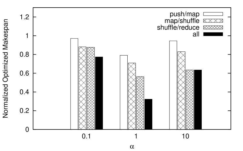
Figure 7: Predicted normalized makespan for optimized plans with various barrier configurations and different values of $\alpha$. All makespans are normalized relative to the optimal makespan for an all-global-barrier configuration. Each bar represents the phase boundary at which the global barrier is relaxed to pipelining, with “all” corresponding to an all-pipelining configuration.

Now we study the impact of relaxing barriers on the makespan predicted by our model. In particular, we focus on the impact of using pipelining vs. global barriers at each phase boundary. In Figure 7, we show the normalized makespan for a select set of different barrier configurations. All predicted makespan values shown in the figure are normalized relative to the optimal makespan derived for an all-global-barrier configuration, i.e., one which has a global barrier at each phase boundary. The bars in the figure show the effect of relaxing only a single global barrier to pipelining at a time, at the push/map, the map/shuffle, and the shuffle/reduce boundaries respectively, as well as the all-pipelined configuration, where all barriers are pipelined. We make two key observations.

• When phases are roughly “balanced” in terms of time taken, pipelining is most effective. This is because overlapping the execution of two balanced phases gives more opportunity for reducing their total execution time, compared to when one phase significantly dominates the other. For the parameters considered here, the phases are most closely balanced when $\alpha=1$, as can be seen from Figure 6. Consequently, we see from Figure 7 that each barrier relaxation provides the greatest benefit when $\alpha=1$.

• Relaxing late-stage barriers—such as those between map and shuffle or between shuffle and reduce—is predicted to have a greater benefit than relaxing barriers between push and map stages. The reason is that our optimization is more constrained in data placement during the shuffle phase than the push phase due to the one-reducer-per-key constraint, and hence pipelining finds more opportunity to hide the latency of the shuffle phase with its adjoining computational phases (map or reduce). This phenomenon can also be observed from Figure 6, where we see that the shuffle time is higher than the push time with our optimization (e2e multi), particularly for $\alpha$=1 and 10.

To summarize, relaxing barriers is most useful when the execution phases are roughly balanced, and for later phase boundaries, where there is more opportunity for latency hiding over the optimal plan with global barriers.

4.5 Distribution of network resources

To evaluate the effect of distribution of network resources, we derive optimized execution plans using our proposed (end-to-end multi-phase) optimization algorithm for all of the network environments described in Section 4.1, starting from a relatively homogeneous environment with a single data center, to an intra-continental setup consisting of two data centers in the US, to globally-distributed setups with four or eight data centers.

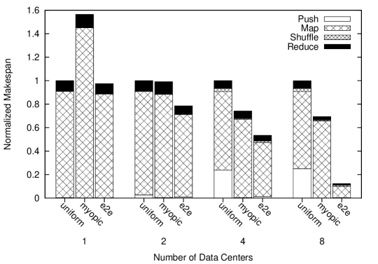
(a) $\alpha$=0.1

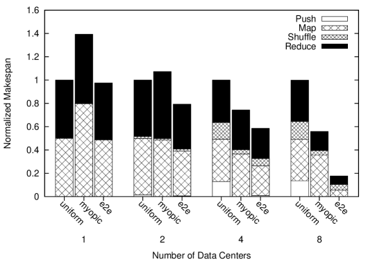
(b) $\alpha$=1

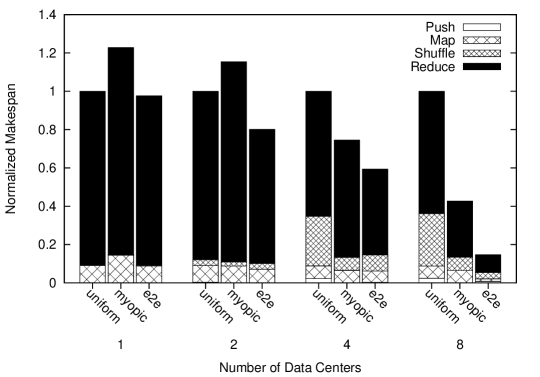
(c) $\alpha$=10

Figure 8: A comparison of myopic and end-to-end optimization relative to the uniform baseline for different network environments and different values of $\alpha$. The makespans are normalized by computing the ratio of the actual makespan to the makespan of the corresponding uniform schedule. A global barrier is used between phases in all cases.

Figure 8 shows the makespan for the myopic optimization that successively optimizes the execution times of the push phase and the shuffle phase and the end-to-end optimization that optimizes makespan by considering all phases at once. Both the myopic and end-to-end optimizations are compared against a baseline that performs uniform push and shuffle.

If the network environment is a single data center with relative homogeneity of compute rates and network bandwidths, the uniform baseline does almost as well as end-to-end optimization for all values of $\alpha$. Note that this provides supporting evidence for why Hadoop’s use of a largely uniform schedule is quite effective in homogeneous environments. Interestingly, some optimization is worse than none, as myopic optimization does worse than uniform. Intuitively, myopic optimization reacts to rectify small communication imbalances, but this can in turn create larger computational imbalances among the map and reduce tasks, resulting in a longer makespan. This effect can be seen from the figure by the increased map and reduce times for myopic for $\alpha$=0.1 and 10 respectively.

As the network environment becomes more diverse with more and more data centers, both myopic and end-to-end optimizations start to perform better than uniform, as uniform fails to account for the diversity of the environment. As expected, end-to-end performs the best with makespans that are smaller by 82-87% over uniform and by 65-82% over myopic.

In summary, our results show that our optimization derives much greater opportunity for improvement as the diversity and heterogeneity of the environment increases, while reducing to a largely uniform placement for tightly-coupled, homogeneous environments, where myopic optimization may actually hurt performance.

4.6 Comparing our optimization to Hadoop

We compare the results of our optimization against vanilla Hadoop, which represents a typical unmodified Hadoop execution.

4.6.1 Experimental setup

For these experiments, we use the 8-node cluster with the emulated links bandwidths of the distributed PlanetLab environment as described in Section 3.2. Each of our eight physical nodes hosts two map slots and one reduce slot, as well as an HDFS datanode. Each physical node also runs a simple TCP server to act as a data source. We use our modified Hadoop implementation described in Section 3.1, using largely default Hadoop configuration options, aside from increasing io.sort.mb to 200 and increasing the Java heap size for worker processes to 800$\,\mathrm{MB}$. We also set
dfs.replication to 1 to prevent replication over emulated slow links, which can have a pronounced adverse impact on performance (See Section 4.6.5). Since the emulated environment exhibits no inherent hierarchical structure, there is no direct way to model it using Hadoop’s rack-oriented model. Therefore, for Hadoop’s network topology configuration, we use the default that models each node as being co-located in the same rack.

To focus our comparison on the efficacy of our optimized plans, we implement the push phase for both vanilla Hadoop and our optimization using the same type of InputSplit as described in Section 3.1. To provide vanilla Hadoop with a competitive baseline, we take advantage of Hadoop’s existing data-locality optimization, using the getLocations method of our InputSplit to hint that Hadoop should push data from a data source to the most local compute node. In our testbed, since map tasks run on the same physical nodes as our data sources, we hint that Hadoop should move data locally from the data source server directly into the local HDFS data node. This is logically identical to Hadoop’s existing data-locality optimization, but applied to the emulated wide-area setting. In addition, we allow vanilla Hadoop to use its dynamic mechanisms such as speculative task execution and non-local work stealing to avoid stragglers and idle resources.

For our optimization, we provide our modified Hadoop implementation with the exact plans produced by our optimization. The optimized plan is derived using the model parameters for the underlying platform and the application, and the model uses a G-P-L barrier configuration at the consecutive phase boundaries to capture Hadoop’s execution behavior. In order to ensure that Hadoop strictly follows these plans, we turn on our LocalOnly configuration option (see Section 3.1). Further, to understand the benefit of our offline execution plan, we turn off Hadoop’s dynamic mechanisms mentioned above for our optimization. As a baseline, we also compare vanilla Hadoop and our optimization to a uniform execution plan, which uniformly pushes and shuffles data to mappers and reducers respectively.

4.6.2 Applications

We implement three MapReduce applications for this evaluation, which vary in terms of their application characteristics, particularly, the expansion factor $\alpha$:

(1) Word Count. This application takes as input a set of documents and produces as output, for each term in the set, the number of occurrences of that term. Map tasks receive a plain text document and tokenize it, then count the number of occurrences of each term. For each term $t$, the mapper emits the key-value pair $(t,f(t))$ where $f(t)$ denotes the number of times term $t$ occurred. We apply the in-mapper-combining pattern, described by Lin and Dyer [21]. Reducers receive key-value pairs of the form $(t,[f(t)])$ where $t$ is the term and $[f(t)]$ denotes a list of all counts for that term. The reducer simply sums up this list and emits as final output a tuple with $t$ as the key, and the sum of all counts as the value. This application exhibits high aggregation; $\alpha=0.09$. As inputs for this application, we use plain-text eBooks from Project Gutenberg [13]. The total input size is roughly 16.5$\,\mathrm{GB}$, spread across 48,000 eBooks.

(2) Sessionization. This application takes as input a collection of Web server logs and produces as output, for each user, the sequence of “sessions” for that user. At its core, this application is a large distributed sort. Here the map function receives a single server log entry $v$, which it then parses into a user identifier $id$ and timestamp $t$. As intermediate data, mappers emit the composite key $(id,t)$ along with the unchanged value $v$. This application uses a custom SortComparator to sort first by $id$, then by $t$. Intermediate key-value pairs are grouped using a custom GroupingComparator that groups only on the $id$; all log entries for a single $id$ are then presented to a single call of the reduce function. The system ensures that these values are delivered in sorted order by timestamp $t$, and the reduce function simply determines the boundary between sessions for that user by looking for sufficiently large gaps in this value. There is no opportunity for aggregating (or expanding) intermediate results in this application, as the mapper simply routes data to reducers. Therefore $\alpha=1.0$. We use a portion of the WorldCup98 trace [3] (roughly 5$\,\mathrm{GB}$ spanning 60 million log entries) as the input data for this application.

(3) Full Inverted Index. This application takes as input a collection of documents, each represented as a pair of document identifier $id$ along with a sequence of word identifiers $w$. It produces as output, for each word $w$, the complete list of documents in which that word occurs, as well as the position within those documents. The implementation is modeled after the example from Lin and Dyer [21]. This application also uses a custom SortingComparator and GroupingComparator to rely as much as possible on the underlying MapReduce system for its data movement. This application expands the input data by adding additional information regarding each term to the index, yielding $\alpha=1.88$. As input, we use the same set of eBooks as for the Word Count application, but preprocessed to remove stop words, and replace terms with an integer term identifier; in essence a simple forward index. This data again spans 48,000 books, but the more concise representation yields a total input size of roughly 4$\,\mathrm{GB}$.

4.6.3 Experimental results

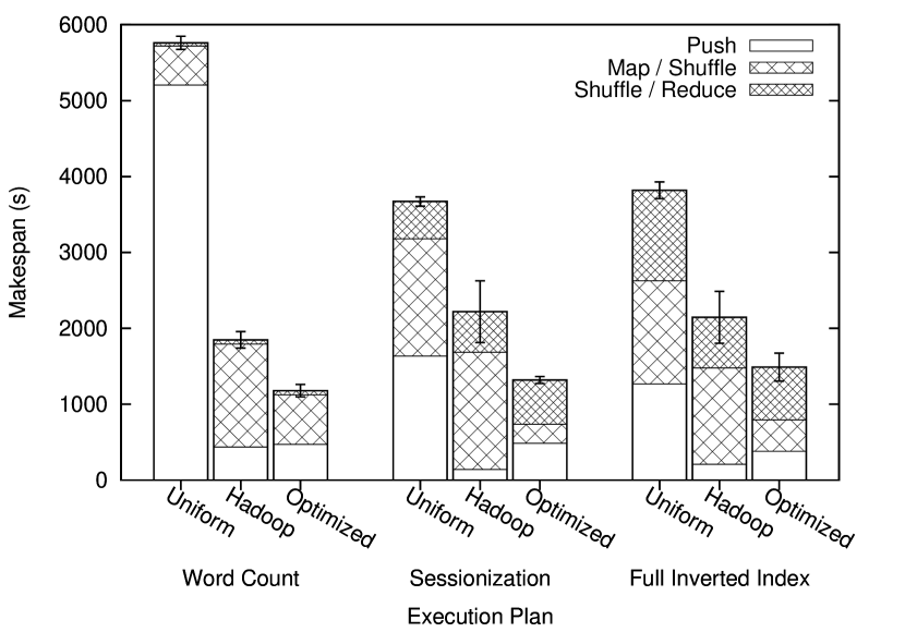
Figure 9: Actual makespan for three sample applications on our local testbed. Error bars reflect 95% confidence intervals.

Figure 9 shows the results of our comparison for the three applications. Note that for Hadoop, since the shuffle phase is partially overlapped with the map and reduce phases, we depict only three phases in each bar in the graph: the push phase, the overlapped map/shuffle phases, and the overlapped shuffle/reduce phases. We see that across all applications, while vanilla Hadoop substantially outperforms the uniform execution plan (by 68, 40, and 44% for Word Count, Sessionization, and Full Inverted Index respectively), Hadoop executing our optimized plan achieves a further improvement of 36, 41, and 31% over vanilla Hadoop for the same applications. Further, we see how vanilla Hadoop makes myopic decisions. Hadoop reduces the push time substantially (by 92, 91, and 83% for Word Count, Sessionization, and Full Inverted Index, respectively) over uniform. However, our optimization, while increasing the push time over vanilla Hadoop, achieves more significant reduction in end-to-end makespan than vanilla Hadoop by better optimizing the map, shuffle, and reduce phases. Thus, overall, we find that Hadoop executing our offline end-to-end, multi-phase optimal execution plan outperforms vanilla Hadoop using its dynamic mechanisms.

4.6.4 Enhancing optimized plan dynamically

Our optimization provides an offline execution plan based on information about the underlying infrastructure available before the job begins execution. As mentioned above, Hadoop provides two dynamic mechanisms to modify the initial execution plan based on the observed runtime behavior of the network and nodes: (i) speculative task execution, where another copy of a straggler task is launched on a different node; and (ii) work stealing, where a node may request a non-local task if that node is idle. Here, we evaluate the benefit of using dynamic mechanisms in addition to the static execution plan derived from the results of our optimization.

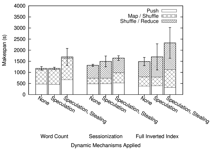
Figure 10: Effect of Hadoop’s dynamic scheduling mechanisms applied atop our optimized static execution plan for three sample applications. Error bars reflect 95% confidence intervals.

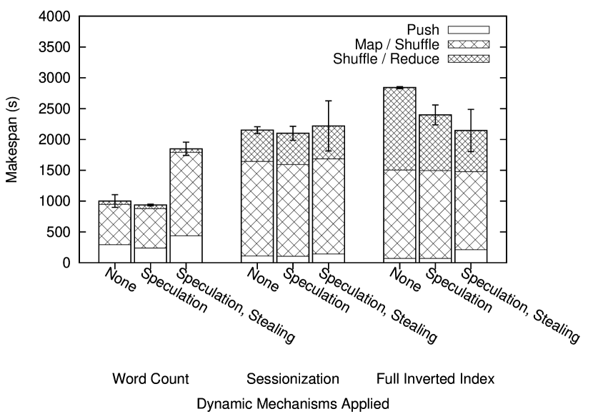
Figure 11: Effect of Hadoop’s dynamic scheduling mechanisms applied atop a competitive Hadoop baseline plan, one that pushes from each data source to the most local mapper, and distributes intermediate keys uniformly across all reducers. Error bars reflect 95% confidence intervals.

Figure 10 shows the impact of enabling these two dynamic mechanism on the performance of the optimized plan for each of the three sample applications. Additionally, Figure 11 shows the impact of enabling these mechanisms atop a competitive Hadoop baseline plan. We find from these two figures that, applied on its own, speculation does not statistically significantly degrade performance in any case, while it significantly improves performance in one case. On the other hand, the addition of work stealing to speculation never statistically significantly improves performance over speculation alone, while in some cases—specifically Word Count—stealing significantly degrades performance. In fact, there is only one case where the combination of speculation and stealing is statistically significantly better than the static baseline: Full Inverted Index with the Hadoop baseline. The reason in this case is that the static plan myopically optimizes the push phase, adversely impacting the much more dominant shuffle and reduce phases. By enabling speculation and optionally stealing, however, Hadoop is able to bypass the bottleneck network links and compute nodes by moving data over faster links and placing tasks on faster nodes.

Although the dynamic mechanisms are helpful in such a case, they can also degrade performance in other cases. For example, the combination of speculation and stealing statistically significantly worsens performance for two of the three applications when applied atop an optimized plan, and for one of the three applications when applied atop a Hadoop baseline plan. For the optimized plans, this occurs because dynamic changes to the offline plan can actually undermine the optimization. After all, if the computed plan is optimal, then barring any changes to the underlying infrastructure, no dynamic change could improve performance. For the Hadoop baseline, the degradation occurs for the Word Count application, for which the runtime is dominated by the push and map phases. For such an application, Hadoop’s myopic optimization is actually quite effective, and dynamically deviating from this plan can yield significantly worse performance as we see here.

Though it is not shown directly in the figures, it is noteworthy that the best Hadoop performance is never statistically significantly better than the performance with the optimized plan. Hadoop’s best performance relative to the optimized plan occurs for the Word Count application, for which Hadoop with speculation (but not stealing) yields a lower mean makespan than the optimized plan, but not statistically significantly so.

These results overall show the strength of the statically enforced optimized plan. At the same time, they show how dynamic mechanisms can improve performance when the initial plan is far from optimal, as is the case for the Full Inverted Index application with the Hadoop baseline. Such a situation could also arise if network or node conditions were to change significantly, for example due to network congestion or changes in background CPU load. Developing dynamic mechanisms that improve performance in such cases without adversely affecting the performance in other cases is an interesting direction for future work.

4.6.5 Impact of data replication across slow links

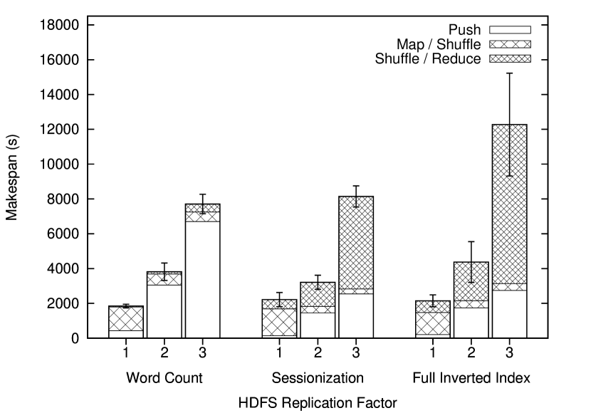
Figure 12: Effect of HDFS file replication for three sample applications. Error bars reflect 95% confidence intervals.

In our model, we restrict replication to be intra-cluster, to avoid sending redundant data across slow wide-area links. Figure 12 shows the impact of wide-area replication on the performance of vanilla Hadoop for each of the three applications. As the figure shows, increasing replication substantially increases the cost of data push, as well as the cost of the reduce phase due to the need to materialize final results to the distributed file system. While higher replication also yields a reduction in compute time in the map phase due to greater scheduling flexibility, this improvement is dwarfed by the increased communication costs. However, replication across clusters would be useful for achieving higher fault tolerance against geographically localized faults. Such replication may also provide other opportunities for performance optimization; e.g., work stealing may be directed to local tasks to avoid high-overhead data communication. Enhancing our model to incorporate cross-cluster replication, or complementing our execution with other techniques such as checkpointing for intermediate data [18] is an interesting direction for future work.

5 Related Work

MapReduce implementations [10, 14] have traditionally been deployed over a tightly-coupled cluster or data center, comprising largely homogeneous compute resources connected over a local-area network. Several research efforts have shown the impact on performance of MapReduce if this assumption is broken. Heterogeneity [30] in terms of node speeds was shown to have an adverse impact on the default MapReduce scheduling performance. Mantri [2] further shows the impact of heterogeneity in terms of machine and network characteristics as well as application workload on the performance of MapReduce within a data center environment. Tarazu [1] provides techniques for dynamic load balancing and reducing network burstiness within a tightly-coupled cluster of heterogeneous compute nodes. Our model is able to incorporate such heterogeneity in computation and communication characteristics, not only within a single data center, but also over a highly-distributed environment. Further, some of these dynamic techniques can be applied at the data center level, and are complementary to our model’s outputs, which provide an initial execution plan for a geographically distributed environment.

Our recent work [7] has shown the performance impact on MapReduce in a highly distributed environment, and explored multiple architectural choices for deploying MapReduce based on network and application characteristics. Hierarchical MapReduce [22] adds a new “Global Reduce” stage to the MapReduce semantics to aggregate results from a MapReduce job executed across multiple clusters, though it avoids the issue of costly data push by assuming data is small or already present in the local clusters. In this paper, we present a more general analytic approach to explore some of these tradeoffs, and our optimization provides the best execution plan based on system characteristics. Kim et al. [17] consider Hadoop performance in an inter-cloud environment, focusing on minimizing the end time of the shuffle phase, whereas our end-to-end, multi-phase optimization focuses on minimizing the makespan of the entire job.

Most existing work has examined the performance of MapReduce execution after the push phase. We explicitly model the push phase, which is particularly important due to the presence of multiple data sources in our environment. Most MapReduce implementations rely on a distributed file system, such as GFS [12] or HDFS [27], from which mapper nodes can pull their inputs. The presence of a distributed file system also implicitly imposes a global barrier between the push and map phases, where the mappers do not start execution until all the input data has already been placed in the distributed file system. Hadoop effectively allows pipelining between the push and map phase and coarse-grained pipelining between the map and shuffle phases (see Subsection 3.1.4). MapReduce Online [9] proposes finer-grained pipelining of the map and shuffle phases, as well as pipelining between MapReduce jobs. Verma et al. [28] propose system changes to relax Hadoop’s local shuffle/reduce barrier. This affects the semantics of the reduce phase, and they present techniques for transforming applications to support this change. Our model captures all these variations and enables us to compare the performance of these choices across different phase boundaries.

Our model is data-oblivious; i.e., it does not assume knowledge of the input data contents, but such knowledge could be exploited to further improve performance. SkewReduce [19] presents the problem of application-specific computational skew, where different parts of the input data may require different amounts of computation resources. Such data-dependent compute requirements can be incorporated in our model by using data-dependent $C_{i}$ values. CoHadoop [11] co-locates related data on the same node to improve performance of certain applications. Such an approach requires detailed knowledge of input data, which our model does not assume.

Other work has focused on scheduling or fine-tuning MapReduce parameters to provide better performance. Sandholm et al. [26] present a dynamic priority-based system for providing differentiated service to multiple MapReduce jobs. Quincy [16] is a framework for scheduling concurrent jobs to achieve fairness while improving data locality. Our focus is on optimizing the performance of individual job execution in a more distributed environment. Recent work [5] has proposed methods for automatically fine-tuning Hadoop parameters to optimize job performance. Our work takes a different approach, where we attempt to abstract away specific implementation details, so that our model is general enough to capture the abstraction behind many existing implementations. Thus, our model is useful for comparing different design and architectural choices, and some of its recommendations could be instantiated via some of the existing work.

Elastisizer [15] and STEAMEngine [6] focus on MapReduce provisioning within a cloud environment. While Elastisizer uses offline profiling along with black-box and white-box models to select the right cluster size, STEAMEngine uses both offline and online job profiling along with dynamic scaling to provision and place the jobs. The focus of these works is on largely homogeneous cluster environments, as opposed to multi-cluster environments like ours. Further, provisioning is a complementary problem to the problem of performance optimization within a given computation environment, addressed in this paper.

Fault tolerance in Hadoop has been addressed by increasing the availability of intermediate data [18]. MOON [20] explored MapReduce performance in a local-area volunteer computing environment and extended Hadoop to provide improved performance under low reliability conditions. While our focus in this paper is on performance, achieving fault tolerance over a highly distributed environment is an interesting area of future work.

6 Concluding Remarks

In this paper, we addressed the problem of executing MapReduce in a highly distributed environment, comprising distributed data sources and computational resources. We developed a modeling framework to capture MapReduce execution in such a distributed environment. This framework is flexible enough to capture several design choices and performance optimizations for MapReduce execution. We proposed a model-driven optimization that has two key features: (i) it is end-to-end as opposed to myopic optimizations that may only make locally optimal but globally suboptimal decisions, and (ii) it can control multiple MapReduce phases to achieve low runtime, as opposed to single-phase optimizations that may control only individual phases. Our model results showed that our optimization can provide nearly 82% and 64% reduction in execution time over myopic and the best single-phase optimizations, respectively. We modified Hadoop to implement our model outputs, and using three different MapReduce applications over an 8-node emulated PlanetLab testbed, we showed that our optimized Hadoop execution plan achieves 31-41% reduction in runtime over a vanilla Hadoop execution. Our model-driven optimization also provided several insights into the choice of techniques and execution parameters based on application and platform characteristics. For instance, we found that an application’s data expansion factor $\alpha$ can influence the optimal execution plan significantly, both in terms of which phases of execution are impacted more and where pipelining is more helpful. Our results also showed that as the network becomes more distributed and heterogeneous, our optimization provides higher benefits (82% for globally distributed sites vs. 37% for a single local cluster over myopic optimization), as it can exploit heterogeneity opportunities better.

References

- [1] F. Ahmad, S. T. Chakradhar, A. Raghunathan, and T. N. Vijaykumar. Tarazu: optimizing MapReduce on heterogeneous clusters. In Proceedings of ASPLOS, 2012.
- [2] G. Ananthanarayanan, S. Kandula, A. Greenberg, I. Stoica, Y. Lu, and B. Saha. Reining in the outliers in map-reduce clusters. In Proceedings of OSDI, 2010.
- [3] M. Arlitt and T. Jin. Workload Characterization of the 1998 World Cup Web Site. Technical Report HPL-1999-35R1, HP Labs, Sept. 1999.
- [4] M. Armbrust, A. Fox, R. Griffith, A. D. Joseph, R. H. Katz, A. Konwinsky, G. Lee, D. A. Patterson, A. Rabkin, I. Stoica, and M. Zaharia. Above the clouds: A berkeley view of cloud computing. Technical Report UCB/EECS-2009-28, Electrical Engineering and Computer Sciences, University of California at Berkeley, February 2009.
- [5] S. Babu. Towards automatic optimization of MapReduce programs. In Proceedings of ACM SoCC, 2010.
- [6] M. Cardosa, P. Narang, A. Chandra, H. Pucha, and A. Singh. STEAMEngine: Driving MapReduce Provisioning in the Cloud. In Proceedings of HiPC, 2011.
- [7] M. Cardosa, C. Wang, A. Nangia, A. Chandra, and J. Weissman. Exploring MapReduce Efficiency with Highly-Distributed Data. In The Second International Workshop on MapReduce and its Applications (MAPREDUCE ‘11), June 2011.
- [8] B. Chun, D. Culler, T. Roscoe, A. Bavier, L. Peterson, M. Wawrzoniak, and M. Bowman. PlanetLab: an overlay testbed for broad-coverage services. ACM SIGCOMM Computer Communication Review, 33(3):3–12, July 2003.
- [9] T. Condie, N. Conway, P. Alvaro, J. M. Hellerstein, K. Elmeleegy, and R. Sears. MapReduce Online. In Proceedings of NSDI, 2010.
- [10] J. Dean and S. Ghemawat. Mapreduce: Simplified data processing on large clusters. In Proceedings of OSDI, 2004.
- [11] M. Y. Eltabakh, Y. Tian, F. Özcan, R. Gemulla, A. Krettek, and J. McPherson. CoHadoop: flexible data placement and its exploitation in hadoop. Proc. VLDB Endow., 4:575–585, June 2011.
- [12] S. Ghemawat, H. Gobioff, and S.-T. Leung. The google file system. In SOSP, pages 29–43. ACM, 2003.
- [13] Free eBooks by Project Gutenberg. http://www.gutenberg.org/.
- [14] Hadoop. http://hadoop.apache.org.
- [15] H. Herodotou, F. Dong, and S. Babu. No one (cluster) size fits all: automatic cluster sizing for data-intensive analytics. In Proceedings of ACM SoCC, pages 18:1–18:14, 2011.
- [16] M. Isard, V. Prabhakaran, J. Currey, U. Wieder, K. Talwar, and A. Goldberg. Quincy: fair scheduling for distributed computing clusters. In SOSP, 2009.
- [17] S. Kim, J. Won, H. Han, H. Eom, and H. Y. Yeom. Improving Hadoop performance in intercloud environments. SIGMETRICS Perform. Eval. Rev., 39(3):107–109, Dec. 2011.
- [18] S. Ko, I. Hoque, B. Cho, and I. Gupta. Making Cloud Intermediate Data Fault-Tolerant. In Proceedings of ACM SoCC, 2010. \balancecolumns
- [19] Y. Kwon, M. Balazinska, B. Howe, and J. Rolia. Skew-resistant parallel processing of feature-extracting scientific user-defined functions. In Proceedings of ACM SoCC, 2010.
- [20] H. Lin, X. Ma, J. Archuleta, W.-c. Feng, M. Gardner, and Z. Zhang. MOON: MapReduce On Opportunistic eNvironments. In Proceedings of HPDC, 2010.
- [21] J. Lin and C. Dyer. Data-Intensive Text Processing with MapReduce. Morgan and Claypool Publishers, 2010.
- [22] Y. Luo, Z. Guo, Y. Sun, B. Plale, J. Qiu, and W. W. Li. A hierarchical framework for cross-domain MapReduce execution. In Proceedings of ECMLS, 2011.
- [23] E. Nygren, R. Sitaraman, and J. Sun. The akamai network: A platform for high-performance internet applications. ACM SIGOPS Operating Systems Review, 44(3):2–19, 2010.
- [24] S. Rao, R. Ramakrishnan, A. Silberstein, M. Ovsiannikov, and D. Reeves. Sailfish: A framework for large scale data processing. Technical Report YL-2012-002, Yahoo! Labs, 2012.
- [25] Barnes & Noble - Cross-channel Analytics for Deeper Customer Insights. http://www.asterdata.com/customers/barnes-and-noble.php.
- [26] T. Sandholm and K. Lai. Mapreduce optimization using dynamic regulated prioritization. In ACM SIGMETRICS/Performance, 2009.
- [27] K. Shvachko, H. Kuang, S. Radia, and R. Chansler. The hadoop distributed file system. In 2010 IEEE 26th Symposium on Mass Storage Systems and Technologies (MSST), pages 1–10. IEEE, 2010.
- [28] A. Verma, N. Zea, B. Cho, I. Gupta, and R. H. Campbell. Breaking the MapReduce stage barrier. Cluster Computing, IEEE International Conference on, 0:235–244, 2010.
- [29] H. Williams. Model building in mathematical programming. Wiley, 1999.
- [30] M. Zaharia, A. Konwinski, A. D. Joseph, R. H. Katz, and I. Stoica. Improving mapreduce performance in heterogeneous environments. In Proceedings of OSDI, 2008.