Dynamics of Magnetized Bulk Viscous Strings in Brans-Dicke Gravity

Abstract

We explore locally rotationally symmetric Bianchi I universe in Brans-Dicke gravity with self-interacting potential by using charged viscous cosmological string fluid. We use a relationship between the shear and expansion scalars and also take the power law for scalar field as well as self-interacting potential. It is found that the resulting universe model maintains its anisotropic nature at all times due to the proportionality relationship between expansion and shear scalars. The physical implications of this model are discussed by using different parameters and their graphs. We conclude that this model corresponds to an accelerated expanding universe for particular values of the parameters.

Keywords: Brans-Dicke theory; Scalar field; Cosmic expansion.
PACS: 98.80.-k; 04.50.Kd

1 Introduction

Current observational measurements obtained from many astronomical experiments (like Supernova (Ia), WMAP, SDSS, galactic cluster emission of X-rays, large scale structure and weak lensing etc.) strengthened the picture of cosmic expansion at an accelerating rate [1]-[4]. This significant phenomenon of cosmic expansion is prompted by dark energy (DE), a mysterious unusual kind of matter containing negative pressure. This is inconsistent with the strong energy condition and plays a dominant role in the composition of our universe [5]. The investigation of its obscure nature is one of the most fascinating issues in modern cosmology. Consequently, enormous DE proposals including Chaplygin gas, quintom, k-essence, phantom, quintessence, cosmological constant etc. have been suggested [6, 7]. However, none of them provides an unambiguous solution to this problem and thus leaving it as a mystery for the researchers.

General Relativity, in spite of its success in many ways, remained unsuccessful for describing the reality of DE and some other cosmological issues. This suggested the exploration of alternative theories of gravity by taking some modifications in Einstein Hilbert action [8, 9]. For this purpose, numerous modified gravity theories like Gauss-Bonnet theory, scalar tensor theories, $f(R)$ and $f(T)$ gravities and recently, $f(R,T)$ gravity theory etc. have been constructed [10, 11]. Among these modified theories, scalar-tensor theories are the most viable and interesting candidates of DE. In scalar tensor theories, the gravity effects are discussed by a tensor as well as a scalar field [12]-[14]. There are different scalar tensor theories available in literature, including the scalar tensor theories formulated by Brans and Dicke, Lyra, Nordtvedt and Wagoner, Saez and Ballester which are of particular interest [12, 13],[15]-[18].

Brans-Dicke (BD) gravitational theory is the most prominent and prevailing case of scalar-tensor theories which provides convenient solutions to many cosmological issues such as universe inflation and its late time behavior, coincidence problem, cosmic acceleration etc [19, 20]. Dynamical gravitational constant $(G=\frac{1}{\phi})$, non-minimal interaction of scalar field with geometry, compatibility with the Dirac’s large number and Mach’s hypotheses as well as weak equivalence principle are some major facets of this theory [12]-[14]. Various versions of BD theory are available in literature like generalized and chameleonic BD theory etc. for different cosmological implications. Brans-Dicke formalism attracted many researchers to explore exact cosmological universe models for cosmic expansion [21]-[23]. Recently, we have investigated exact solution of the BD field equations by using perfect, anisotropic and magnetized anisotropic fluids as matter contents [24].

According to grand unified theories, the phase transition (caused by the reduction in the temperature below some critical temperature in the initial epochs of the universe evolution) results in the creation of some topological defects including domain walls and cosmic strings etc. These defects are responsible for density fluctuations and hence lead to a precise description of structure formation [25]. Since the cosmic strings interact with gravity, therefore it would be worthwhile to canvas the string’s gravitational and astrophysical consequences. The study of magnetic field effects in the matter distribution is of considerable interest as it provides an effective way to understand the initial phases of cosmic evolution. Bulk viscous effects in the fluid lead to negative energy field and hence have a significant impact on the dynamics of the universe [26, 27]. Thus the study of magnetized cosmic stings under the influence of bulk viscosity leads to a better understanding of the dynamics of the universe. Various string cosmological universe models have been investigated in general relativity and scalar tensor theories [28]-[30].

This paper deals with the exact BD universe model with magnetized viscous cosmic strings. The paper is designed in the following layout. Next section provides BD formulation in the presence of self-interacting potential for Locally Rotationally Symmetric (LRS) Bianchi type I (BI) universe model and bulk viscous clouds of strings with electromagnetic effects. In section 3, we construct the universe model by solving the field equations. We discuss various physical parameters for the universe model. Lastly, we present a summary of the obtained results.

2 LRS Bianchi I Model and BD Formulation

In a simple BD theory, the BD coupling parameter remains as a constant, while its modified versions can be obtained by introducing variable BD parameter, i.e., $\omega(\phi)$ and a self-interacting potential term. In Jordon frame, the action for self-interacting BD theory [24] is specified by

$$S=\int d^{4}x\sqrt{-g}[L_{\phi}+L_{m}].$$ (1)

Here $L_{m}$ is the matter contribution and $L_{\phi}$ is the Lagrangian density having BD scalar field $\phi$ as source and is given by

$$L_{\phi}=\phi R-\frac{\omega}{\phi}\phi^{,\alpha}\phi_{,\alpha}-U(\phi),$$ (2)

where $\omega$ is the BD coupling parameter (which is taken to be constant), $R$ is the Ricci scalar and $U(\phi)$ represents self-interacting potential. The self-interacting BD equations obtained by varying the action with respect to scalar and tensor fields and are given by

$$G_{\mu\nu} = \frac{1}{\phi}[\phi_{,\mu;\nu}-g_{\mu\nu}\Box\phi]+\frac{\omega}{\phi^{2}}[\phi_{,\mu}\phi_{,\nu}-\frac{1}{2}g_{\mu\nu}\phi_{,\alpha}\phi^{,\alpha}]$$ (3)

$$- \frac{U(\phi)}{2\phi}g_{\mu\nu}+\frac{T_{\mu\nu}}{\phi},$$

$$\Box\phi = \frac{T}{3+2\omega}+\frac{1}{3+2\omega}[\phi\frac{dU(\phi)}{d\phi}-2U(\phi)].$$ (4)

Equation (4) provides the evolution of scalar field. Here $T$ and $\Box$ represent the trace of the energy-momentum tensor and the de’Alembertian operator, respectively. This theory leads to other modified theories when BD coupling constant takes some particular values [31, 32]. In the limit, $\phi=\phi_{0},~{}\omega\rightarrow\infty$ and $T\neq 0$, the respective action and hence the field equations of GR could be recovered [33, 34].

In order to investigate the universe formation and the initial epochs of cosmic expansion, the study of Bianchi universe models is of great significance [35, 36]. The LRS BI universe model, as the simplest generalization of FRW universe model, is described by an anisotropic spacetime exhibiting spatial homogeneity [37]

$$ds^{2}=dt^{2}-A^{2}(t)dx^{2}-B^{2}(t)(dy^{2}+dz^{2}).$$ (5)

Here the expansion in $x$ direction is measured by the scale factor $A$, while in $y$ and $z$ directions it is measured by the scale factor $B$. The corresponding field equations (3) become

$$\frac{2\dot{A}\dot{B}}{AB}+\frac{\dot{B}^{2}}{B^{2}}=-(\frac{\dot{A}}{A}+2\frac{\dot{B}}{B})\frac{\dot{\phi}}{\phi}+\frac{\omega}{2}\frac{\dot{\phi}^{2}}{\phi^{2}}+\frac{U(\phi)}{2\phi}+\frac{T_{00}}{\phi},$$ (6)

$$2\frac{\ddot{B}}{B}+\frac{\dot{B}^{2}}{B^{2}}=-2\frac{\dot{B}}{B}\frac{\dot{\phi}}{\phi}-\frac{\omega}{2}\frac{\dot{\phi}^{2}}{\phi^{2}}-\frac{\ddot{\phi}}{\phi}+\frac{U(\phi)}{2\phi}-\frac{T_{11}}{\phi},$$ (7)

$$\frac{\ddot{B}}{B}+\frac{\ddot{A}}{A}+\frac{\dot{A}\dot{B}}{AB}=-(\frac{\dot{A}}{A}+\frac{\dot{B}}{B})\frac{\dot{\phi}}{\phi}-\frac{\omega}{2}\frac{\dot{\phi}^{2}}{\phi^{2}}-\frac{\ddot{\phi}}{\phi}+\frac{U(\phi)}{2\phi}-\frac{T_{22}}{\phi}.$$ (8)

The BD scalar wave equation yields

$$\ddot{\phi}+3(\frac{\dot{A}}{A}+2\frac{\dot{B}}{B})\dot{\phi}=\frac{T}{2\omega+3}-\frac{(2\dot{\phi}U(\phi)-\phi\dot{U})}{(2\omega+3)\dot{\phi}}.$$ (9)

It is interesting to mention here that the energy conservation, $T^{\mu\nu}_{;\mu}=0$, leads to a linearly dependent equation as it is an outcome of covariant divergence of the BD equations (3) and (4). Thus we leave it and take the field equations (6)-(9) only.

The average scale factor, the mean and directional Hubble parameters are

$$a(t)=(AB^{2})^{1/3},\quad H(t)=\frac{1}{3}(\frac{\dot{A}}{A}+2\frac{\dot{B}}{B}),$$ (10)

$$H_{x}=\frac{\dot{A}}{A},\quad H_{y}=H_{z}=\frac{\dot{B}}{B}.$$ (11)

The anisotropy measure of expansion $\Delta$, volume $V$, expansion scalar $\Theta$, deceleration parameter $q$ as well as shear scalar $\sigma$ can be written as

$$\Delta = \frac{1}{3}\sum^{3}_{i=1}(\frac{H_{i}-H}{H})^{2},\quad V=a^{3}(t)=AB^{2},$$ (12)

$$\Theta = u^{\alpha}_{;\alpha}=\frac{\dot{A}}{A}+2\frac{\dot{B}}{B},\quad q=\frac{d}{dt}(\frac{1}{H})-1,\quad\sigma=\frac{1}{\sqrt{3}}(\frac{\dot{A}}{A}-\frac{\dot{B}}{B}).$$ (13)

Here $\Delta=0$ corresponds to isotropic expansion of the universe model.

3 Model for the Magnetized Viscous Cosmic String Fluid

In this section, we discuss BI model with electromagnetic bulk viscous cloud of strings as background fluid distribution given by the energy-momentum tensor [27]

$$T^{\nu}_{\mu}=(\rho+P_{eff})u^{\nu}u_{\mu}-P_{eff}\delta^{\nu}_{\mu}-\lambda x^{\nu}_{\mu}+E^{\nu}_{\mu},$$ (14)

where $u^{\mu}$ is the particle’s four velocity, $\lambda$ is the string tension density, $E^{\nu}_{\mu}$ denotes the electromagnetic part of energy-momentum tensor and $x^{\mu}$ is the spacelike unit vector that provides the string direction. Here we take $u^{\mu}=(1,0,0,0)$ and $x^{\mu}=(0,A^{-1},0,0)$ which satisfy the relations

$$u^{\mu}u_{\mu}=1=-x^{\mu}x_{\mu},\quad u^{\mu}x_{\mu}=0.$$

The effective pressure $P_{eff}$ is defined as the sum of isotropic and viscous pressures, i.e., $P_{eff}=P_{I}+P_{vis}$. We consider here the dust case, i.e., $P_{I}=0$. Moreover, $P_{vis}=-\xi\Theta$, where $\xi$ denotes the bulk viscosity coefficient. The electromagnetic part of $T^{\nu}_{\mu}$ is given by

$$E^{\nu}_{\mu}=\overline{\mu}[|h|^{2}(u_{\mu}u^{\nu}+1/2\delta^{\nu}_{\mu})-h_{\mu}h^{\nu}],$$ (15)

where $h_{\mu}$ is the magnetic flux vector

$$h_{\mu}=\frac{\sqrt{-g}}{2\overline{\mu}}\epsilon_{\mu\nu\alpha\beta}F^{\alpha\beta}u^{\nu},$$ (16)

the terms $\overline{\mu},~{}F^{\alpha\beta}$ and $\epsilon_{\mu\nu\alpha\beta}$ denote the magnetic permeability, the electromagnetic field tensor and the Levi-Civita tensor, respectively. Moreover, $\rho$ represents the proper density of strings being the sum of the particle density $\rho_{p}$ (as the particles are attached to these strings) and string tension density $\lambda$ is specified by $\rho=\rho_{p}+\lambda$.

We assume that the magnetic field is generated in $yz$ plane as its source is the electric current that flows in $x$ direction. Here the magnetic flux vector has only one non-zero component $h_{1}$. Moreover, the assumption of infinitely large conductivity along with finite current (in magnetohydrodynamics limit) leads to $F_{10}=F_{20}=F_{30}=0$ [38]. Thus, all the electromagnetic field tensor components vanish except $F_{23}$. Using Maxwell’s equations

$$F_{\alpha\beta;\rho}+F_{\beta\rho;\alpha}+F_{\rho\alpha;\beta}=0,\quad F^{\alpha\beta}_{;\rho}=0,$$

we find $F_{23}=\Pi$, a constant. The matter tensor (14) has the trace $T=\rho+\lambda-3\xi\Theta$. The non-zero component of magnetic flux vector will be $h_{1}=\frac{\Pi}{\overline{\mu}B}$, yielding the corresponding components of $E^{\nu}_{\mu}$

$$E^{0}_{0}=E^{1}_{1}=\frac{-\Pi^{2}}{2\overline{\mu}B^{4}}=-E^{2}_{2}=-E^{3}_{3}.$$

There are seven unknowns namely $\phi,~{}U,~{}A,~{}B,~{}\rho,~{}\lambda,~{}\xi$ and only three independent field equations. For a closed set of equations, we take the following assumptions:

• $A=B^{n};~{}n\neq 1$, this condition is constructed by setting the ratio $\frac{\sigma}{\Theta}$ as constant, i.e., we assume the proportional relationship between the expansion and shear scalar [39]-[42].

• $\phi=\phi_{0}B^{\delta}$, a well-known power law relationship which indicates that the evolution of BD scalar field $\phi$ is dependent on the scale factor. Moreover, $\delta>0$ for expanding solutions [24].

• $U=U_{0}\phi^{k}$, a power law ansatz for potential in which $k$ is any non-zero integer which can further be written as $U=U_{0}B^{k\delta}$.

• Also, we take $\xi\Theta=M_{1}$, by setting the expansion scalar inversely proportional to bulk viscosity coefficient [27] which means that the rate of cosmic expansion decreases as the viscosity increases. Here $M_{1}$ is any positive constant.

The field equations for the fluid (14) turn out to be

$$(2n+1)\frac{\dot{B}^{2}}{B^{2}} = -(n+2)\frac{\dot{B}}{B}\frac{\dot{\phi}}{\phi}+\frac{\omega}{2}\frac{\dot{\phi}^{2}}{\phi^{2}}+\frac{U(\phi)}{2\phi}+\frac{\rho}{\phi}-\frac{\Pi^{2}}{2\overline{\mu}B^{4}\phi},$$ (17)

$$2\frac{\ddot{B}}{B}+\frac{\dot{B}^{2}}{B^{2}} = -2\frac{\dot{B}}{B}\frac{\dot{\phi}}{\phi}-\frac{\omega}{2}\frac{\dot{\phi}^{2}}{\phi^{2}}-\frac{\ddot{\phi}}{\phi}+\frac{U(\phi)}{2\phi}+\frac{\xi\Theta}{\phi}+\frac{\lambda}{\phi}-\frac{\Pi^{2}}{2\overline{\mu}B^{4}\phi},$$

$$(n+1)\frac{\ddot{B}}{B}+n^{2}\frac{\dot{B}^{2}}{B^{2}} = -(n+1)\frac{\dot{B}}{B}\frac{\dot{\phi}}{\phi}-\frac{\omega}{2}\frac{\dot{\phi}^{2}}{\phi^{2}}-\frac{\ddot{\phi}}{\phi}+\frac{U(\phi)}{2\phi}+\frac{\xi\Theta}{\phi}$$ (19)

$$+ \frac{\Pi^{2}}{2\overline{\mu}B^{4}\phi},$$

$$\ddot{\phi}+(n+2)\frac{\dot{B}}{B}\dot{\phi} = \frac{(\rho+\lambda+3\xi\Theta)}{(2\omega+3)}+\frac{(\phi\dot{U}-2\dot{\phi}U(\phi))}{(2\omega+3)\dot{\phi}},$$ (20)

where we have used $A=B^{n}$.

Now there are three independent field equations and three unknowns namely $\rho,~{}B$ and $\lambda$. Equation (19) yields

$$2\ddot{B}+\frac{(2n(n+\delta)+(\omega_{0}+2)\delta^{2})\dot{B}^{2}}{(n+\delta+1)B} = \frac{2M_{1}B^{(1-\delta)}}{\phi_{0}(\delta+n+1)}+\frac{\Pi^{2}B^{-(\delta+3)}}{\overline{\mu}\phi_{0}(\delta+n+1)}$$

$$+ \frac{U_{0}B^{(\delta k-\delta+1)}}{\phi_{0}(\delta+n+1)}$$

whose solution is

$$\dot{B}^{2} = \frac{2M_{1}B^{(2-\delta)}}{\phi_{0}(\delta+n+1)(2-\delta+s)}-\frac{\Pi^{2}B^{-(\delta+2)}}{\overline{\mu}\phi_{0}(\delta+n+1)(\delta+2-s)}$$ (21)

$$+ \frac{U_{0}B^{(\delta k+2-\delta)}}{\phi_{0}(\delta+n+1)(\delta k+2-\delta+s)}+\frac{M_{2}}{B^{s}},$$

where $M_{2}$ is a constant of integration (taken to be positive) and $s$ is a constant given by

$$s=\frac{2n(n+\delta)+(\omega+2)\delta^{2}}{(n+\delta+1)}.$$

Equation (21) leads to

$$dt = [\frac{2M_{1}B^{(2-\delta)}}{\phi_{0}(\delta+n+1)(2-\delta+s)}-\frac{\Pi^{2}B^{-(\delta+2)}}{\overline{\mu}\phi_{0}(\delta+n+1)(\delta+2-s)}$$ (22)

$$+ \frac{U_{0}B^{(\delta k+2-\delta)}}{\phi_{0}(\delta+n+1)(\delta k+2-\delta+s)}+\frac{M_{2}}{B^{s}}]^{-1/2}dB.$$

Introducing the notions $B=\tau$ for time and $X,~{}Y,~{}Z$ for the space coordinates, the corresponding BI universe model becomes

$$ds^{2} = [\frac{2M_{1}\tau^{(2-\delta)}}{\phi_{0}(\delta+n+1)(2-\delta+s)}-\frac{\Pi^{2}\tau^{-(\delta+2)}}{\overline{\mu}\phi_{0}(\delta+n+1)(\delta+2-s)}$$ (23)

$$+ \frac{U_{0}\tau^{(\delta k+2-\delta)}}{\phi_{0}(\delta+n+1)(\delta k+2-\alpha+s)}+\frac{M_{2}}{\tau^{s}}]^{-1}d\tau^{2}-\tau^{2n}dX^{2}$$

$$- \tau^{2}(dY^{2}+dZ^{2}).$$

Equation (17) yields the density as

$$\rho(B)=[(1+2n)+\delta(n+2)-\frac{\omega\delta^{2}}{2}]\phi_{0}\dot{B}^{2}B^{(\delta-2)}+\frac{U_{0}B^{2}}{2}+\frac{\Pi^{2}}{2\overline{\mu}B^{4}}.$$

Substituting the value from Eq.(21), it follows that

$$\rho(\tau) = \phi_{0}(1+2n+\delta(n+2)-\frac{\omega\delta^{2}}{2})\frac{M_{2}}{\tau^{s-\delta+2}}+[(1+2n+\delta(n+2)$$ (24)

$$- \frac{\omega\delta^{2}}{2})\frac{2M_{1}}{(\delta+n+1)(2-\delta+s)}]-[\frac{(1+2n+\delta(n+2)-\frac{\omega\delta^{2}}{2})}{(\delta+n+1)(2+\delta-s)}$$

$$- \frac{1}{2}]\frac{\Pi^{2}}{\overline{\mu}\tau^{4}}-[\frac{1}{2}-\frac{(1+2n+\delta(n+2)-\frac{\omega\delta^{2}}{2})}{(\delta+n+1)(\delta k+2+s-\delta)}]U_{0}\tau^{\delta k}.$$

The string tension density $\lambda$ can be expressed from Eqs.(LABEL:16) and (20) as

$$\lambda(\tau) = \frac{(3+2\omega)\phi_{0}\tau^{\delta}}{(4+2\omega)}[\frac{2\ddot{\tau}}{\tau}+(1+\frac{\omega\delta^{2}}{2}+n\delta+4\delta)\frac{\dot{\tau}^{2}}{\tau^{2}}-\frac{U_{0}\tau^{\delta(k-1)}}{\phi_{0}(3+2\omega)}$$ (25)

$$\times (1+2\omega+k)-\frac{M_{1}(6+2\omega)}{(3+2\omega)\phi_{0}\tau^{\delta}}+\frac{\Pi^{2}}{2\overline{\mu}\tau^{\delta+4}\phi_{0}}]-\frac{\rho}{4+2\omega},$$

where

$$\frac{\ddot{\tau}}{\tau} = \frac{1}{(\delta+n+1)}[\frac{M_{1}(2-\delta)\tau^{-\delta}}{\phi_{0}(s+2-\delta)}-\frac{(\delta+2)\Pi^{2}\tau^{-(\delta+4)}}{2\overline{\mu}\phi_{0}(s-\delta-2)}$$

$$+ \frac{U_{0}(\delta(k-1)+2)\tau^{\delta(k-1)}}{2\phi_{0}(\delta(k-1)+2+s)}],$$

$\rho$ is given by Eq.(24) and $\frac{\dot{\tau}^{2}}{\tau^{2}}$ can be calculated from Eq.(21).

The density of the particles is

$$\rho_{p}=\rho-\lambda = -\frac{\rho(5+2\omega)}{4+2\omega}-\frac{(3+2\omega)\phi_{0}\tau^{\delta}}{4+2\omega}[\frac{2\ddot{\tau}}{\tau}+(1+\frac{\omega\delta^{2}}{2}$$ (26)

$$+ n\delta+4\delta)\frac{\dot{\tau}^{2}}{\tau^{2}}-\frac{U_{0}\tau^{\delta(k-1)}}{\phi_{0}(3+2\omega)}(1+2\omega+k)$$

$$- \frac{M_{1}(6+2\omega)}{(3+2\omega)\phi_{0}\tau^{\delta}}+\frac{\Pi^{2}}{2\overline{\mu}\tau^{\delta+4}\phi_{0}}].$$

The directional Hubble, mean Hubble and deceleration parameters become

$$H_{x}=nH_{y} = nH_{z}=n[\frac{2M_{1}\tau^{-\delta}}{\phi_{0}(\delta+n+1)(2-\delta+s)}-\frac{\Pi^{2}(\delta+n+1)^{-1}}{\overline{\mu}\phi_{0}(\delta+2-s)}$$

$$\times \tau^{-(\delta+4)}-\frac{U_{0}\tau^{(k-1)\delta}}{\phi_{0}(\delta+n+1)(k\delta-\delta+s)}+\frac{M_{2}}{\tau^{(s+2)}}]^{1/2},$$

$$H = \frac{(n+2)}{3}[\frac{2M_{1}\tau^{-\delta}}{\phi_{0}(\delta+n+1)(2-\delta+s)}-\frac{\Pi^{2}(\delta+n+1)^{-1}}{\overline{\mu}\phi_{0}(\delta+2-s)}$$

$$\times \tau^{-(\delta+4)}-\frac{U_{0}\tau^{(k-1)\delta}}{\phi_{0}(\delta+n+1)(k\delta-\delta+s)}+\frac{M_{2}}{\tau^{(s+2)}}]^{1/2},$$

$$q = \frac{3(s+1)}{(n+2)}-1-\frac{3\tau^{2}}{(n+2)(\delta+n+1)\dot{\tau}^{2}}[\frac{M_{1}}{\phi_{0}\tau^{\delta}}+\frac{\Pi^{2}\tau^{-(\delta+4)}}{2\overline{\mu}\phi_{0}}$$

$$+ \frac{U_{0}\tau^{\delta(k-1)}}{2\phi_{0}}].$$

The expansion scalar is

$$\Theta = (n+2)[\frac{2M_{1}\tau^{-\delta}}{\phi_{0}(\delta+n+1)(2-\delta+s)}-\frac{\Pi^{2}\tau^{-(\delta+4)}}{\overline{\mu}\phi_{0}(\delta+n+1)(\delta+2-s)}$$ (27)

$$+ \frac{U_{0}\tau^{(k-1)\delta}}{\phi_{0}(\delta+n+1)(k\delta-\delta+s)}+\frac{M_{2}}{\tau^{(s+2)}}]^{1/2}.$$

The coefficient of bulk viscosity takes the form

$$\xi = \frac{M_{1}}{(n+2)}[\frac{2M_{1}\tau^{-\delta}}{\phi_{0}(\delta+n+1)(2-\delta+s)}-\frac{\Pi^{2}\tau^{-(\delta+4)}}{\overline{\mu}\phi_{0}(\delta+n+1)(\delta+2-s)}$$ (28)

$$+ \frac{U_{0}\tau^{(k-1)\delta}}{\phi_{0}(\delta+n+1)(k-\delta+s)}+\frac{M_{2}}{\tau^{(s+2)}}]^{-1/2}.$$

The shear scalar is

$$\sigma = \frac{(1-n)}{\sqrt{3}}[\frac{2M_{1}\tau^{-\delta}}{\phi_{0}(\delta+n+1)(2-\delta+s)}-\frac{\Pi^{2}\tau^{-(\delta+4)}}{\overline{\mu}\phi_{0}(\delta+n+1)(\delta+2-s)}$$ (29)

$$- \frac{U_{0}\tau^{(k-1)\delta}}{\phi_{0}(\delta+n+1)(k\delta-\delta+s)}+\frac{M_{2}}{\tau^{(s+2)}}]^{1/2}.$$

The volume for the model takes the form $V=\tau^{n+2}$ which is zero initially and becomes divergent when $\tau\rightarrow\infty$ indicating that the expansion of the universe starts from zero to infinite volume. The anisotropic measure of expansion leads to $\Delta=\frac{2(n-1)^{2}}{(n+2)^{2}}$ which is constant (as we have taken the shear scalar proportional to expansion scalar) and it becomes zero for $n=1$. In our case, $n\neq 1$, thus the universe model remains anisotropic throughout the cosmic time. The energy density remains positive for the allowed range of parameters as shown in Figure 1(a). However, it becomes infinite at initial epoch but decreases for final phases of the universe evolution. The energy density approaches to a positive value due to viscosity, given by

$$\rho=\frac{2M_{1}}{(\delta+n+1)(s+2-\delta)}[1+2n-\frac{\omega\delta^{2}}{2}+\delta(n+2)]$$

as $\tau\rightarrow\infty$. If we take viscosity to be negligible, then the density approaches to zero for later times thus representing an empty universe in future.

The string tension density $\lambda$ increases with the passage of time and then remains a constant for future evolution of the universe as shown in Figure 1(b). The particle density $\rho_{p}$ exhibits a similar behavior as does the energy density. It decreases from infinite value (at $\tau=0$) to a certain constant due to viscosity effects and then remains constant for the future evolution as shown in Figure 2(a).

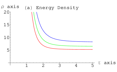
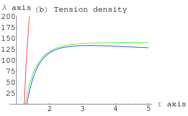
Figure 1: Plots (a) and (b) show the energy density $\rho$ and the string tension density $\lambda$ versus time $\tau$. Here, red, green and blue lines correspond to $\omega=-1.7,~{}-1.8$ and $-1.9$ respectively. Also, we have taken $\delta=2,~{}M_{1}=4,~{}M_{2}=3,~{}n=3,~{}\bar{\mu}=0.5,~{}k=-4,~{}\Pi^{2}=3,~{}U_{0}=1,$ and $\phi_{0}=1$.

The model results in dynamical deceleration parameter and consequently leads to negative as well as positive values for certain choices of parameters. For later time with $k<0,~{}-2<\omega<-1.5,~{}0<\delta<1$ and $n>2$, the deceleration parameter becomes negative, indicating accelerated expanding behavior of the universe model given by

$$q=\frac{3(s+1)}{n+2}-1-\frac{3(2-\delta+s)}{(n+2)(\delta+n+1)}.$$

However, for other choices of parameters, it exhibits decelerating behavior.

The graph of deceleration parameter for particular choices of the parameters is given in Figure 2(b). It is clear that the model represents accelerated expanding universe as the deceleration parameter attains small negative values as shown in this figure.

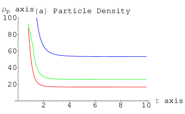
Figure 2: Plot (a) shows the particle density $\rho_{p}$ versus time $\tau$ and (b) indicates the deceleration parameter $q$ versus BD parameter $\omega$. In graph (b), we have taken $n=2$, the blue, green and red lines correspond to $\delta=0.2,~{}0.4$ and $0.6$ respectively.

The graphical illustration for expansion scalar is given in Figure 3(a), while the shear scalar, directional and mean Hubble parameters exhibit a similar behavior. These parameters go to zero when $\tau\rightarrow\infty$ and diverge for initial time indicating the beginning of the universe model with a big bang explosion as shown in Figure 3(a). Figure 3(b) indicates the graphical behavior of viscosity parameter $\xi$ which is opposite to the expansion scalar (in accordance with our assumption). The viscosity parameter is negligible at the initial epoch and increases with the passage of time as shown in Figure 3(b). Hence it prevents the universe to be empty for its future evolution.

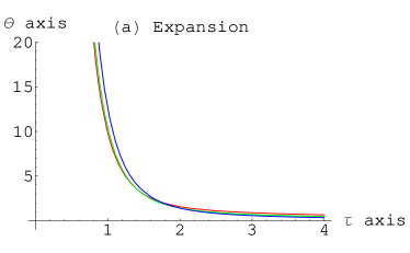
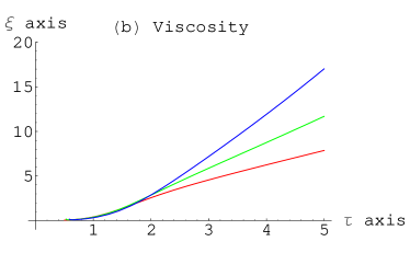
Figure 3: Plots (a) and (b) represent the expansion parameter $\Theta$ and viscosity $\xi$ respectively. Here, $M_{1}=4,~{}M_{2}=3,~{}n=3,~{}\bar{\mu}=0.5,~{}k=-4,~{}\Pi^{2}=3,~{}U_{0}=1,$ and $\phi_{0}=1$. The red, green and blue colors correspond to $\omega=-1.7,~{}-1.8$ and $-1.9$ respectively.

4 Summary

It is argued that magnetic field has cosmological origin as there was highly ionized matter that was coupled to magnetic field which further leads to neutral matter as a consequence of universe expansion. It is interesting to discuss the magnetic field effects on the expansion history of the universe. Moreover, bulk viscosity effects and scalar field have important role for obtaining accelerated expanding universe model. Thus it would be worthwhile to discuss BI universe filled with magnetized bulk viscous strings for the discussion of early and late stages of the universe in scalar tensor theories. This paper investigates the cosmological model in self-interacting BD gravity with magnetized bulk viscous cloud of strings by taking certain physical conditions. All the cosmological parameters depend upon the values of BD parameter $\omega$, parameter $n$ as well as parameter $\delta$ (that appear due to scalar field). We have discussed the resulting model using different physical parameters through graphs. The results are summarized as follows.

• According to Hubble [43], there would have been an infinitely hot and dense universe in its early phase. In fact, all the density of the universe was concentrated at a single point and hence initially there was zero volume of the universe. Penrose and Hawking [44, 45] have argued that expansion of the universe has been started from this dense and hot phase by an explosion and then universe is going to expand till today. After infinite time, universe would have infinite volume with negligible density. In our case, the proper energy density, string tension density as well as particle density remain positive for increasing BD parameter values and cosmic time. At initial epoch, the proper energy and particle densities diverge while they turn out to be finite for later time due to bulk viscous effects. Hence the presence of viscosity prevents the universe to be empty in its future evolution. Clearly, the physical behavior of our constructed model supports these arguments as energy densities turn out to be infinite (divergent) at initial epoch and hence is of considerable interest. However, the string tension density increases with the increase in time and BD parameter values.

• Different parameters like $H,~{}H_{x},H_{y},~{}\Theta$ and $\sigma$ exhibit increasing behavior for decreasing $\tau$ and become divergent at initial epoch indicating the big bang start of the model. However, these parameters approach to zero asymptotically, i.e., $\tau\rightarrow\infty$. Thus the constructed model has an initial singularity. Moreover, scalar field evolves from zero (initially) to infinite value as $\tau\rightarrow\infty$.

• As we have discussed in our previous work [24], in case of BI universe filled with perfect fluid, there is a constant and positive deceleration parameter yielding decelerated expanding universe model. This problem is then resolved by taking anisotropic matter contents. In present work, the deceleration parameter turns out to be a dynamical quantity rather than a constant due to the presence of self-interacting potential, viscosity and magnetic field effects which can provide negative values and hence yields accelerated expansion of universe. For example, if we take $\tau\rightarrow\infty$ and $-2<\omega<-3/2$ as well as decreasing values of scalar field, the deceleration parameter gives negative values lying in the range $-1<q<0$ which is in good agreement with the observed range for cosmic expansion as shown in Figure 2(b).

• The anisotropic measure of expansion of the universe model turns out to be a constant showing that the universe model exhibits anisotropic behavior through the whole range of cosmic time. In [46], it has been pointed out that some large-angle anomalies are seen in CMB radiations, violating the statistical isotropy of the observable universe. For a better description of these anomalies, plane symmetric and homogeneous but anisotropic universe models play a very significant role. Moreover, it is found [47]-[49] that removing a Bianchi component in WMAP data can explain various large-angle anomalies yielding an isotropic universe. Thus the universe may have accomplished a slight anisotropic geometry in cosmological models irrespective of inflation. If the anisotropic nature of the model is maintained through the whole range of time, then it may explain or discuss these large-angle anomalies in CMB radiations.

• The viscosity parameter increases with the passage of time which corresponds to a non-empty universe in future.

• In all physical parameters, the component of magnetic field has a negative contribution, i.e., these physical parameters reduce due to the presence of magnetic field.

In [50], a class of Bianchi II, VII and IX filled with cosmic string fluid within Saez and Ballester gravity is discussed. It is found that the constructed model has no initial singularity which is inconsistent with the big bang model. Likewise, in a new work [51], the same class is discussed with cosmological strings in BD gravity and it is observed that the volume of the universe model is contracting rather than expanding which is physically unacceptable. However, in the present work, no such ambiguity exists and the results are in well agreement with the observations. It is worthwhile to mention here that our results are consistent with those already available in the context of GR [27].

References

- [1] Perlmutter, S. et al.: Nature 391(1998)51.
- [2] Riess, A.G. et al.: Astron. J. 116(1998)1009.
- [3] Bennett, C.L. et al.: Astrophys. J. Suppl. 148(2003)1.
- [4] Tegmark, M. et al.: Phys. Rev. D 69(2004)03501.
- [5] Komatsu, E. et al.: Astrophys. J. Suppl. 180(2009)330.
- [6] Al-Rawaf A.S. and Taha, M.O.: Gen. Relativ. Gravit. 28(1996)935.
- [7] Caldwell, R.R., Dave, R. and Steinhardt, P.J.: Phys. Rev. Lett. 80(1998)1582.
- [8] Briscese, F. et al.: Phys. Lett. B 646(2007)105.
- [9] Bamba, K. et al.: Phys. Rev. D 79(2009)083014.
- [10] Lobo, F.S.N.: arXiv:0807.1640.
- [11] Flanagan, E.E.: Class. Quantum Grav. 21(2004)417.
- [12] Brans, C.H. and Dicke, R.H.: Phys. Rev. 124(1961)925.
- [13] Dirac, P.A.M.: Proc. R. Soc. Lond. A 165(1938)199.
- [14] Weinberg, S.: Gravitation and Cosmology (Wiley, 1972).
- [15] Lyra, G.: Math. Z. 54(1951)52.
- [16] Nordtvedt, K. Jr.: Astrophys. J. 161(1970)1059.
- [17] Wagoner, R.V.: Phys. Rev. D 1(1970)3209.
- [18] Saez, D. and Ballester, V.J.: Phys. Lett. A 113(1985)467.
- [19] Bertolami, O. and Martins, P.J.: Phys. Rev. D 61(2000)064007.
- [20] Banerjee, N. and Pavon, D.: Phys. Rev. D 63(2001)043504.
- [21] Singh, T. and Rai, L.N.: Gen. Relativ. Gravit. 15(1983)875.
- [22] Reddy, D.R.K. and Rao, M.V.S.: Astrophys. Space Sci. 305(2006)183.
- [23] Chakraborty, W. and Debnath, U.: Int. J. Theor. Phys. 48(2009)232.
- [24] Sharif, M. and Waheed, S.: Eur. Phys. J. C 72(2012)1876.
- [25] Zel’sdovich, Y.B., Kokzarev, I.Y. and Okum, L.B.: J. Exp. Theor. Phys. 40(1975)1.
- [26] Misner, C.W.: Astrophys. J. 151(1968)431.
- [27] Tyagi, A. and Sharma, K.: Chin. Phys. Lett. 28(2011)089802.
- [28] Barros, A. and Romero, C.: J. Math. Phys. 36(1995)5800.
- [29] Bali, R. and Yadav, M.K.: Pramana J. Phys. 64(2005)187.
- [30] Pradhan, A.: Fizika B 16(2007)205.
- [31] Sen, S. and Seshadri, T.R.: Int. J. Mod. Phys. D 12(2003)445.
- [32] Sotiriou, T.P. and Faraoni, V.: Rev. Mod. Phys. 82(2010)451.
- [33] Romero, C. and Barros, A.: Phys. Lett. A 173(1993)243.
- [34] Banerjee, N. and Sen, S.: Phys. Rev. D 56(1997)1334.
- [35] Pradhan, A. and Singh, S.K.: Int. J. Mod. Phys. D 13(2004)503.
- [36] Pradhan, A. and Pandey, P.: Astrophys. Space Sci. 301(2006)221.
- [37] Sharif, M. and Zubair, M.: Astrophys. Space Sci. 330(2010)399.
- [38] Maartens, R.: Pramana 55(2000)575.
- [39] Collins, C.B.: Phys. Lett. A 60(1977)397.
- [40] Collins, C.B., Glass, E.N. and Wilkinson, D.A.: Gen. Relativ. Gravit. 12(1980)805.
- [41] Xing-Xiang, W.: Chin. Phys. Lett. 21(2004)1205.
- [42] Yadav, A.K., Pradhan, A. and Singh, A.K.: Astrophys. Space Sci. 337(2012)379.
- [43] Narlikar, J.V.: An Introduction to Cosmology (Cambridge University Press, 2006).
- [44] Hawking, S.: The Illustrated: A Brief History of Time (Bantam Books, 1996).
- [45] Hawking, S.: The Universe in a Nutshell (Bantam Books, 2001).
- [46] Eriksen, H. et al.: Astrophys. J. 605(2004)1420.
- [47] Jaffe, T.R. et al.: Astrophys. J. 629(2005)L1.
- [48] Jaffe, T.R. et al.: Astrophys. J. 643(2006)616.
- [49] Jaffe, T.R. et al.: Astron. Astrophys. 460(2006)393.
- [50] Rao, V.U.M., Santhi, M.V. and Vinutha, T.: Astrophys. Space Sci. 314(2008)73.
- [51] Rao, V.U.M. and Santhi, M.V.: ISRN Math. Phys. (2012).