A search for mass segregation of stars and brown dwarfs in $\rho$ Ophiuchi

Abstract

We apply two different algorithms to search for mass segregation to a recent observational census of the $\rho$ Ophiuchi star forming region. Firstly, we apply the $\Lambda_{\rm MSR}$ method, which compares the minimum spanning tree (MST) of a chosen subset of stars to MSTs of random subsets of stars in the cluster, and determine the mass segregation ratio, $\Lambda_{\rm MSR}$. Secondly, we apply the $m-\Sigma$ method, which calculates the local stellar surface density around each star and determines the statistical significance of the average surface density for a chosen mass bin, compared to the average surface density in the whole cluster. Using both methods, we find no indication of mass segregation (normal or inverse) in the spatial distribution of stars and brown dwarfs in $\rho$ Ophiuchi. Although $\rho$ Ophiuchi suffers from high visual extinction, we show that a significant mass segregation signature would be detectable, albeit slightly diluted, despite dust obscuration of centrally located massive stars.

1 Introduction

Most stars form in groups, clusters, and larger associations. In order to understand the star formation process, it is desirable to quantify the spatial distribution of stars in different star forming regions, so that a clear picture of the formation and evolution of each region can be drawn. It is possible to measure the amount of substructure in a region (e.g.  by using the $\mathcal{Q}$-parameter, Cartwright & Whitworth, 2004) and to quantify the amount of mass segregation (e.g.  the $\Lambda_{\rm MSR}$ method, Allison et al., 2009a, or the $m-\Sigma$ method, Maschberger & Clarke, 2011). Additionally, statistical methods can be applied to find clusters against a background field (e.g. Gutermuth et al., 2009; Schmeja, 2011).

Allison et al. (2009a) found that the amount of mass segregation in the ONC could be quantified by comparing the minimum spanning trees (MSTs) of chosen subsets of stars to the MSTs of random sets of stars. If the MST of the most massive stars is shorter than the MSTs of random subsets of cluster stars, then the cluster is mass segregated. The ONC is mass segregated (see also Hillenbrand & Hartmann, 1998), and the same signature was found by Sana et al. (2010) in Trumpler 14.

However, Parker et al. (2011) found that the most massive stars in the Taurus association were ‘inversely mass segregated’, i.e.  anti-clustered with respect to randomly chosen stars. Is mass segregation therefore a dynamical process (as postulated by Allison et al., 2009b), rather than a primordial outcome of star formation (in hydrodynamical simulations of star cluster formation, primordial mass segregation occurs as part of the competitive accretion process, e.g.  Maschberger et al., 2010, Maschberger & Clarke, 2011)? To answer this question, we must first search for mass segregation in other young star forming regions, ideally using independent methods.

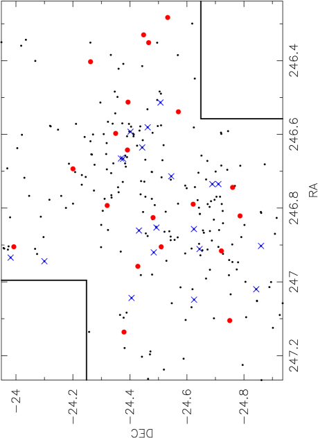
Figure 1: A map of $\rho$ Ophiuchi showing the 255 objects in our dataset (restricted to the WIRCam field). The 20 least massive cluster members (masses up to 0.03 M_⊙) are shown by the blue crosses and the 20 most massive cluster members (masses down to 1.63 M_⊙) are shown by the large red dots. The solid lines indicate the extent of the WIRCam field.

In this paper we search for mass segregation in $\rho$ Ophiuchi. This cluster suffers heavily from differential extinction, so an accurate and self-consistent determination of stellar masses is difficult. However, recent spectroscopic surveys (Alves de Oliveira et al., 2012; Erickson et al., 2011; Geers et al., 2011; Mužić et al., 2012) have probed the low-mass end of the IMF and allowed a complete census of the cluster to be made. We describe the observational sample in Section 2, we describe the methods used to quantify mass segregation in Section 3, we present our results in Section 4, we discuss the results and the potential effects of extinction in Section 5 and we conclude in Section 6.

2 The observational sample

We adopted as a starting point for building the observational sample the most recent census of the $\rho$ Ophiuchi core cluster as compiled in Alves de Oliveira et al. (2012), where a new population of brown dwarf members in the cluster was uncovered and analyzed with respect to the previously known members. Their census includes only stars and brown dwarfs for which there is a spectral type classification and reliable membership confirmation. In short, the compilation takes all the spectroscopically confirmed members compiled for the cluster’s review (see, Wilking et al., 2008, and references therein) in the Handbook of Star Forming Regions (Reipurth, 2008), adding to it the more recent spectroscopic results by Alves de Oliveira et al. (2010); McClure et al. (2010); Geers et al. (2011); Erickson et al. (2011), totalling a list of 250 members where 208 have spectral types earlier than M6, and 42 have spectral types later or equal to M6. At the age of $\rho$ Oph ($\sim$1 Myr), the evolutionary models of the Lyon group (Baraffe et al., 1998; Chabrier et al., 2000) when combined with the temperature scale of Luhman et al. (2003), place the substellar boundary at $\sim$M6.25 (Luhman et al., 2007). We have added to this census two low mass stars and one brown dwarf recently confirmed spectroscopically by Mužić et al. (2012), as well as 3 members where the spectral type carries a larger error (but membership is confirmed) presented by Alves de Oliveira et al. (2012) but not included in their compilation.

In the substellar regime, the spectroscopic follow-up of the CFHT/WIRCam survey (Alves de Oliveira et al., 2012) is nearly complete down to an extinction of 20 visual magnitudes (only 3 photometric candidates were not observed spectroscopically), and within the WIRCam mapped region (interior to the solid lines in Fig. 1). In the stellar domain, a conservative depth of 8 visual magnitudes has been used by Alves de Oliveira et al. (2012) to define a complete sample with spectroscopic confirmation. To complete the database in the stellar domain at higher extinctions, we have included candidate members from X-ray surveys that still lack a spectroscopic confirmation. X-ray surveys of young stellar objects usually have low contamination rates, in particular in clusters like $\rho$ Oph where large amounts of extinction effectively block background sources. From the 51 X-ray sources which lack spectroscopic confirmation compiled in the Wilking et al. (2008) list of candidate members (originally uncovered by Imanishi et al., 2001; Gagné et al., 2004; Ozawa et al., 2005; Pillitteri et al., 2010), 43 are matched to a near-IR source, either in the 2MASS or the WIRCam catalogues. From the remaining 8 X-ray sources, 2 have an uncertain membership status (denoted as x? in Wilking et al., 2008), and 6 are not detected in the J-band, and in any case are outside the photometric completeness limits of the WIRCam survey (J$=$20.5 and H$=$18.9 mag, Alves de Oliveira et al., 2012).

We have used the colour-colour diagram J$-$H vs. H$-$K to deredden each of the X-ray sources along the extinction vector (Rieke & Lebofsky, 1985) and estimate a spectral type by comparing their near-IR photospheric colours to those characteristic of young stellar objects (Luhman et al., 2010, their Table 13). This method could not be applied for 9 sources which have strong IR excess and therefore their position on the colour-colour diagram is likely to be affected by the contribution of the disk, and to 4 sources which although classified as Class III fall in a region of the diagram where the colours of young stellar objects ($\sim$M9 to early L) increase nearly parallel to the reddening vector, and therefore any solution is degenerate. We estimated spectral types ($\sim$K4 to $\sim$M8) for 30 sources using this method.

To estimate the masses of the members of the cluster, we first convert spectral types to temperature, adopting the temperature scale from Schmidt-Kaler (1982) for stars earlier than M0, and the scale from Luhman et al. (2003) for sources with spectral type between M0 and M9.5. For the L dwarfs, we applied the scale proposed by Lodieu et al. (2008) extrapolated to the L4 spectral type. Masses were derived from the 1 Myr evolutionary models (Baraffe et al., 1998; Chabrier et al., 2000; Siess et al., 2000) according to each target’s effective temperature.

Because we derive our masses from temperatures, many stars are assigned the same mass from the stellar models. This is potentially a problem for our mass segregation algorithm, as 25 stars at the peak of the IMF may be assigned the same mass. We therefore apply a small amount of random noise to each mass, thereby making each value unique.

In Fig. 1 we show the 255 objects in our dataset (which we have restricted to the WIRCam field). We plot the 20 most massive stars (masses down to 1.63 M_⊙) as the large red points, and the 20 least massive objects (masses up to 0.03 M_⊙) as the blue crosses.

2.1 Spatially and extinction-limited sample

A major caveat in studying a representative sample of the $\rho$ Ophiuchi population is the variable extinction across the cluster. To attempt to correct our methods for this, we also examined a spatially and extinction limited sample of objects. We selected from the original data base all sources that had in the colour-magnitude diagram H vs. J$-$H an A_V$\lesssim$20 mag (see, for example, Fig. 9 in Alves de Oliveira et al., 2012). The data base limited both spatially and to an extinction of 20 visual magnitudes contains 205 members. Though the masses of the X-ray members determined from photometry are likely to carry a large uncertainty, they represent only $\sim$11$\%$ of this sample, and should nevertheless reflect in relative terms the relation between the real masses.

3 Method

In this section we outline the two methods we use to look for mass segregation signatures in the data, namely the $\Lambda_{\rm MSR}$ ratio pioneered by Allison et al. (2009a) and the $m-\Sigma$ distribution, recently proposed by Maschberger & Clarke (2011).

3.1 The $\Lambda_{\rm MSR}$ mass segregation ratio

We first quantify any mass segregation present in the cluster by using the $\Lambda_{\rm MSR}$ ratio introduced by Allison et al. (2009a). This constructs a minimum spanning tree (MST) between a chosen subset of stars and then compares this MST to the average MST length of many random subsets.

The MST of a set of points is the path connecting all the points via the shortest possible pathlength but which contains no closed loops (e.g. Prim, 1957; Cartwright & Whitworth, 2004).

We use the algorithm of Prim (1957) to construct MSTs in our dataset. We first make an ordered list of the separations between all possible pairs of stars. Stars are then connected together in ‘nodes’, starting with the shortest separations and proceeding through the list in order of increasing separation, forming new nodes if the formation of the node does not result in a closed loop.

We find the MST of the $N_{\rm MST}$ stars in the chosen subset and compare this to the MST of sets of $N_{\rm MST}$ random stars in the cluster. If the length of the MST of the chosen subset is shorter than the average length of the MSTs for the random stars then the subset has a more concentrated distribution and is said to be mass segregated. Conversely, if the MST length of the chosen subset is longer than the average MST length, then the subset has a less concentrated distribution, and is said to be inversely mass segregated (see e.g. Parker et al., 2011). Alternatively, if the MST length of the chosen subset is equal to the random MST length, we can conclude that no mass segregation is present.

By taking the ratio of the average (mean) random MST length to the subset MST length, a quantitative measure of the degree of mass segregation (normal or inverse) can be obtained. We first determine the subset MST length, $l_{\rm subset}$. We then determine the average length of sets of $N_{\rm MST}$ random stars each time, $\langle l_{\rm average}\rangle$. There is a dispersion associated with the average length of random MSTs, which is roughly Gaussian and can be quantified as the standard deviation of the lengths $\langle l_{\rm average}\rangle\pm\sigma_{\rm average}$. However, we conservatively estimate the lower (upper) uncertainty as the MST length which lies 1/6 (5/6) of the way through an ordered list of all the random lengths (corresponding to a 66 per cent deviation from the median value, $\langle l_{\rm average}\rangle$). This determination prevents a single outlying object from heavily influencing the uncertainty. We can now define the ‘mass segregation ratio’ ($\Lambda_{\rm MSR}$) as the ratio between the average random MST pathlength and that of a chosen subset, or mass range of objects:

$$\Lambda_{\rm MSR}={\frac{\langle l_{\rm average}\rangle}{l_{\rm subset}}}^{+{\sigma_{\rm 5/6}}/{l_{\rm subset}}}_{-{\sigma_{\rm 1/6}}/{l_{\rm subset}}}.$$ (1)

A $\Lambda_{\rm MSR}$ of $\sim$ 1 shows that the stars in the chosen subset are distributed in the same way as all the other stars, whereas $\Lambda_{\rm MSR}>1$ indicates mass segregation and $\Lambda_{\rm MSR}<1$ indicates inverse mass segregation, i.e.  the chosen subset is more sparsely distributed than the other stars.

As noted by Allison et al. (2009a), the MST method gives a quantitative measure of mass segregation with an associated significance and it does not rely on defining the centre of a cluster.

There are several subtle variations of $\Lambda_{\rm MSR}$. Olczak, Spurzem & Henning (2011) propose using the geometric mean to reduce the spread in uncertainties, and Maschberger & Clarke (2011) propose using the median MST length to reduce the effects of outliers from influencing the results. However, in the subsequent analysis we will adopt the original $\Lambda_{\rm MSR}$ from Allison.

3.2 The $m-\Sigma$ distribution

Recently, Maschberger & Clarke (2011) proposed a method to analyse mass segregation which measures the distribution of local stellar surface density, $\Sigma$, as a function of stellar mass. We calculate the local stellar surface density following the prescription of Casertano & Hut (1985), modified to account for the analysis in projection. For an individual star the local stellar surface density is given by

$$\Sigma=\frac{N-1}{\pi r_{N}^{2}},$$ (2)

where $r_{N}$ is the distance to the $N^{\rm th}$ nearest neighbouring star (we adopt $N=10$ throughout this work).

If there is mass segregation, massive stars are concentrated in the central, dense region of a cluster and thus should have higher values of $\Sigma$. This can be seen in a plot of $\Sigma$ versus mass, showing all stars and highlighting outliers. Trends in the $m-\Sigma$ plot can be shown by the moving average (or median) of a subset, $\tilde{\Sigma}_{\mathrm{subset}}$, compared to the average (median) of the whole sample, $\tilde{\Sigma}_{\mathrm{all}}$. The signature of mass segregation is then $\tilde{\Sigma}_{\mathrm{subset}}>\tilde{\Sigma}_{\mathrm{all}}$, and of inverse mass segregation $\tilde{\Sigma}_{\mathrm{subset}}<\tilde{\Sigma}_{\mathrm{all}}$. The statistical significance of mass segregation can be established with a two-sample Kolmogorov-Smirnov test of the $\Sigma$ values of the subset against the $\Sigma$ values of the rest.

Note that there are many more ways of defining mass segregation. For instance, one can choose a cluster centre and measure the mass function as a function of radial distance (Gouliermis et al., 2004; Sabbi et al., 2008), or the distance of the most massive star(s) from the cluster centre compared to the average distance of low-mass stars to the cluster centre (Kirk & Myers, 2011). Both methods rely on determining the centre of the cluster or association, which in the case of low-number clusters with substructure is non-trivial and is virtually impossible in the case of a highly substructured region such as Taurus (Parker et al., 2011).

4 Results

In this section we present the results of our $\Lambda_{\rm MSR}$ analysis, followed by the $m-\Sigma$ distribution. We then discuss the effects of extinction on the results.

4.1 $\Lambda_{\rm MSR}$ for high mass stars

In Fig. 2 we show the evolution of $\Lambda_{\rm MSR}$ as a function of the number of stars in an MST, $N_{\rm MST}$ for the most massive stars in the cluster. We increase the number of stars in the MST in steps of 6, which is a compromise between a high enough resolution to pick out structure between different mass regimes, and a low enough resolution so that we do not add noise to the plot. The first subset compares the MST of the 20 most massive stars to the median of many different random sets of 20 stars, and the second subset is the 26 most massive stars compared to the median of random sets of 26 stars, and so on. On the top axis we also indicate the mass of the least massive star within that value of $N_{\rm MST}$, at regular intervals.

Fig. 2 we see that there is no clear mass segregation signature (normal or inverse) in the most massive stars in the cluster (the most massive 20 stars are indicated by the large red points in Fig. 1). The 20 most massive stars (with masses above 1.63 M_⊙) have a mass segregation ratio $\Lambda_{\rm MSR}=0.89^{+0.09}_{-0.13}$, which does deviate from $\Lambda_{\rm MSR}=1$ (indicating slight inverse mass segregation), but because the 26 most massive stars are consistent with $\Lambda_{\rm MSR}=1$, this result is not particularly significant.

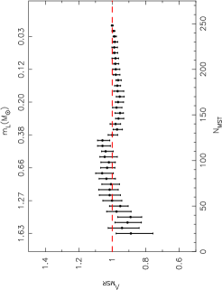
Figure 2: The evolution of the mass segregation ratio, $\Lambda_{\rm MSR}$, for the $N_{\rm MST}$ most massive stars in our dataset and we also indicate the lowest mass star, $m_{\rm L}$ within the $N_{\rm MST}$. Error bars show the 1/6 and 5/6 percentile values from the median, as described in the text. The dashed line indicates $\Lambda_{\rm MSR}=1$, i.e.  no mass segregation.

4.2 $\Lambda_{\rm MSR}$ for low mass stars

In Fig. 3 we show the evolution of $\Lambda_{\rm MSR}$ as a function of the number of stars in an MST, $N_{\rm MST}$ for the least massive stars in the cluster. We begin by constructing an MST with the 20 least massive objects in the cluster, and then increasing the number of objects in the MST by 6 at each stage. On the top axis we now indicate the mass of the most massive star within the $N_{\rm MST}$ subset.

We see that the least massive objects do not show any strong mass segregation signature, and (within the uncertainties) are consistent with $\Lambda_{\rm MSR}=1$.

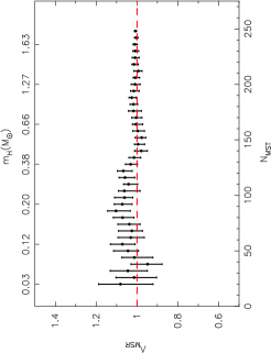
Figure 3: The evolution of the mass segregation ratio, $\Lambda_{\rm MSR}$, for the $N_{\rm MST}$ least massive stars in our dataset and we also indicate the highest mass star, $m_{\rm H}$ within the $N_{\rm MST}$. Error bars show the 1/6 and 5/6 percentile values from the median, as described in the text. The dashed line indicates $\Lambda_{\rm MSR}=1$, i.e.  no mass segregation.

4.3 The $m-\Sigma$ distribution

We show the $m-\Sigma$ distribution for the stars in our dataset in Fig. 4. The upper (black) dashed line is the mean $\Sigma$ value for the whole cluster, and the lower (blue) dashed line is the median value. We also show the mean and median $\Sigma$ values for the 50 most massive stars (on the righthand side) and the 50 least massive stars (on the lefthand side) by the solid lines.

The plot shows that the mean and median $\Sigma$ values of the lowest mass objects in the cluster are marginally higher than for the whole sample. The $p$-values of a two-sample KS test ($\Sigma$ of low-mass stars versus the entire cluster) are $p=0.21$ (20 least massive) and $p=0.51$ (50 least massive). Usually, these would need to be smaller than $p=0.05$ at a significance level corresponding to $2\sigma$, in order to reject the hypothesis of “no mass segregation”. Thus, the lowest mass objects are not mass segregated.

The most massive stars lie at slightly lower $\Sigma$ values compared to the whole cluster, suggesting inverse mass segregation. Here the $p$-values are $p=0.17$ and $p=0.70$ for the 50 and 20 most massive stars, respectively. Again, this does not indicate any significant deviation of the spatial distribution of the massive stars from the spatial distribution of the other stars. The 50 most massive stars are inversely mass segregated, similar to the $\Lambda_{\rm MSR}$ results, but only at a $1\sigma$ level. This is not the case for the 20 most massive stars, where no inverse mass segregation can be concluded. Given the small $n$ and the rather weak signature for $\Lambda_{\rm MSR}$ this result can be deemed compatible with the $\Lambda_{\rm MSR}$.

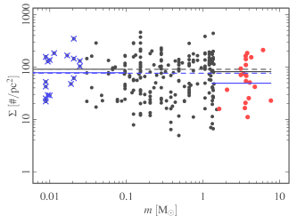
Figure 4: The $m-\Sigma$ distribution for the stars in our dataset. We plot the local surface density for each star against its mass. We then determine the median (blue lines) and mean (black lines) $\Sigma$ for the entire cluster (the dashed lines) and for the 50 least massive, and 50 most massive stars in the cluster (the solid lines).

4.4 Extinction-limited sample

A major caveat in determining the spatial distribution of a sample of objects in $\rho$ Ophiuchi is the variable extinction across the cluster. As a check that our results do not change when an extinction limit is imposed on the data, we apply an $A_{v}$ limit of 20 mag and then repeat the MST and $m-\Sigma$ analysis on this extinction-limited sample. We find no discernible difference to the results in either case; i.e.  there is no clear mass segregation signature in either the high- or low-mass objects in the cluster.

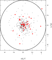
(a) No mass segregation

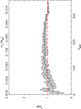
(b) No mass segregation

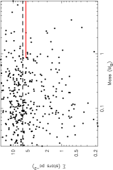
(c) No mass segregation

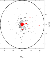
(d) Mass segregation

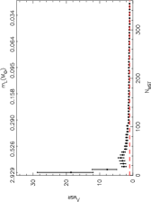
(e) Mass segregation

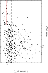
(f) Mass segregation

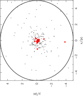
(g) Mass segregation with extinction

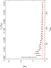
(h) Mass segregation with extinction

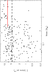
(i) Mass segregation with extinction

Figure 5: Results for a fake cluster without mass segregation (panels a – c), with mass segregation (d – f), with mass segregation but some stars removed due to high extinction (g – i). In each case we show the morphology of the cluster (the most massive stars are shown by the large red dots), the plot of $\Lambda_{\rm MSR}$ for the high mass stars, and the $m-\Sigma$ plot. The extent of the extinction cloud is shown by the black circle. in the $m-\Sigma$ plots the median $\tilde{\Sigma}$ value for the most massive stars is shown by the solid red line, and the median $\tilde{\Sigma}$ value for the whole cluster is shown by the dashed line.

5 Discussion

The results presented in Section 4 show that there is no evidence of mass segregation in that the most massive stars are not centrally concentrated, as they are in e.g. the ONC (Allison et al., 2009a) and Trumpler 14 (Sana et al., 2010). This could indicate that mass segregation may be a dynamical process, rather than a primordial outcome of star formation, but a study of more star forming regions is required to substantiate this hypothesis.

In this dynamical scenario, the massive stars form at random locations in a substructured cluster, and then a subvirial collapse facilitates mass segregation on a very short timescale ($\sim$ 1 Myr, Allison et al., 2009b). $\rho$ Oph is not substructured (Cartwright & Whitworth, 2004), but may have been at earlier ages. If it was substructured at earlier ages, this has not facilitated dynamical mass segregation in this cluster.

5.1 Extinction

The high level of extinction makes observing objects in $\rho$ Oph challenging, and it is possible that even with our extinction-limited sample, some stars are still hidden in the centre of the cluster. In such a scenario, unobserved high mass stars could reside in the central regions, and any mass segregation of such stars would not be observed. In this case, both our mass segregation-finding algorithms would erroneously give a null-result, similar to those described in the previous Section.

Here, we conduct a simple numerical experiment to determine how much a mass segregation signature could be diluted by high levels of extinction, such as that present in $\rho$ Oph. We distribute 360 stars randomly in a Plummer sphere (Plummer, 1911), with a half-number radius of 1 pc according to the prescription in Aarseth, Hénon & Wielen (1974), and assign masses (again at random) from a 3-part Kroupa (2002) IMF of the form:

$$N(M)\propto\left\{\begin{array}[]{ll}M^{-0.3}\hskip 11.38092ptm_{0}<M/{\rm M_{\odot}}\leq m_{1}\,,\\ M^{-1.3}\hskip 11.38092ptm_{1}<M/{\rm M_{\odot}}\leq m_{2}\,,\\ M^{-2.3}\hskip 11.38092ptm_{2}<M/{\rm M_{\odot}}\leq m_{3}\,,\end{array}\right.$$ (3)

and we choose $m_{0}$ = 0.02 M_⊙, $m_{1}$ = 0.1 M_⊙, $m_{2}$ = 0.5 M_⊙, and $m_{3}$ = 10 M_⊙. In Fig. 5(a) we show the morphology of this cluster, with the 40 most massive stars shown by the red points. If we determine $\Lambda_{\rm MSR}$ for the most massive stars (in steps of 6 objects) we see that this cluster is not mass segregated, with $\Lambda_{\rm MSR}\simeq 1$ throughout (Fig. 5(b)). The $m-\Sigma$ algorithm also shows no significant differences between the 40 most massive stars and the cluster as a whole (the solid red line and the dashed line, respectively, shown in Fig. 5(c)).

We apply a simple mass segregation algorithm to the Plummer sphere by swapping the positions of the 40 most central stars with the positions of the 40 most massive stars (we choose 40 stars to clearly demonstrate the effects of extinction in Fig. 5, but the results are similar for the 20 most massive stars). We show the new spatial configuration of the massive stars in the cluster in Fig. 5(d). Several of the most massive stars are originally within the sample of the 40 most central stars, and end up (randomly) being assigned positions outside the central core. In one sense, such a configuration is perhaps more realistic than if the 40 most massive stars were also the 40 most central; in a real cluster dynamical interactions between the central stars would likely eject one or two of the massive stars.

In Fig. 5(e) we show the evolution of $\Lambda_{\rm MSR}$ as a function of the number of stars in the MST. The effect of artificially mass segregating the cluster is clearly seen, with $\Lambda_{\rm MSR}=18.6^{+10.2}_{-6.7}$. The cluster shows significant mass segregation down to the $40^{\rm th}$ most massive star, which has $\Lambda_{\rm MSR}=3.6^{+1.3}_{-0.9}$. Similarly, the $m-\Sigma$ method also shows that the cluster is mass segregated; in Fig. 5(f) we show the median surface density of the entire cluster by the dashed line ($\tilde{\Sigma}=6.35$ stars pc^-2) and the median surface density of the 40 most massive stars by the red solid line ($\tilde{\Sigma}=10.76$ stars pc^-2). A two-sample KS test returns a p-value of $<10^{-8}$ that the two distributions could be drawn from the same parent population.

We now assign a power-law extinction to the fake cluster, from the centre out to a radius of 5 pc (denoted by the circle in Figs 5(a), 5(d) and 5(g)). We then assign an $A_{v}$ value to each star using the following formula:

$$A_{v}(r)=20\left[1-\left(\frac{|r|}{5\,{\rm pc}}\right)^{5/3}\right],$$ (4)

where $r$ is the position of the star with respect to the cluster centre and $|r|$ is the modulus of its vector. To account for projection effects along the line of sight, we double $A_{v}(r)$ if the $z$-component of the vector $r$ is negative. Therefore, in the central regions of the cluster, the $A_{v}$ value can range between $\sim 10-40$. We then remove all stars with $A_{v}>20$, leaving a total of 193 stars. In Fig. 5(g) we show the spatial distribution of the remaining objects.

Once again, we calculate $\Lambda_{\rm MSR}$ for the remaining objects, and Fig. 5(h) shows that the mass segregation signature is still observable, although to a lesser extent due to the removal of several of the most massive stars in the cluster. The peak value is now $\Lambda_{\rm MSR}=6.4^{+3.4}_{-3.0}$, but the plot still shows the same morphology as the non-extinction-limited data-sample. Furthermore, the $m-\Sigma$ method also shows that the cluster is still mass segregated; in Fig. 5(i) we show the median surface density of the entire cluster by the dashed line ($\tilde{\Sigma}=4.50$ stars pc^-2) and the median surface density of the 40 most massive stars by the red solid line ($\tilde{\Sigma}=7.34$ stars pc^-2). A two-sample KS test returns a p-value of $<10^{-2}$ that the two distributions could be drawn from the same parent population.

We have demonstrated with a simple model for extinction that the two mass segregation finding algorithms could still determine whether a cluster suffering from extinction is significantly mass segregated or not. The results suggest that the actual dataset, whilst possibly lacking some cluster members due to obscuration, is likely reflecting the true spatial distribution of stars and brown dwarfs in $\rho$ Oph.

6 Conclusions

We have used an observational census of $\rho$ Ophiuchi, which was recently enhanced by several surveys probing the substellar domain of the IMF, to search for possible mass segregation signatures in the spatial distribution of stars and brown dwarfs in this cluster.

We have utilised two different algorithms. Firstly, we used the $\Lambda_{\rm MSR}$ technique (Allison et al., 2009a), which compares the minimum spanning tree (MST) of a chosen subset of stars, to the MSTs of randomly chosen stars in the cluster. If the MST length of a chosen subset is shorter than the MST length of the random objects, then the cluster is mass segregated. Secondly, we have used the $m-\Sigma$ plot, which compares the local surface density surrounding massive stars to the the average surface density of all of the stars in the cluster. By this definition, a cluster is mass segregated if the massive stars have a significantly higher than average surface density. Our conclusions are as follows:

(i) The $\Lambda_{\rm MSR}$ technique finds that the most massive stars show hints of being inversely mass segregated, with $\Lambda_{\rm MSR}=0.89^{+0.09}_{-0.13}$ for the 20 most massive stars. However, $\Lambda_{\rm MSR}$ is consistent with there being no mass segregation of the 26 most massive stars, and so on. The least massive stars show no clear deviation from $\Lambda_{\rm MSR}=1$.
(ii) The $m-\Sigma$ distribution also suggests that the most massive stars may be inversely mass segregated (but with no strong statistical significance), and with no difference in the distribution of low-mass stars compared to the cluster average.
(iii) The high levels of extinction in $\rho$ Oph may mean that some members are missing from the dataset. However, we have demonstrated that a significant difference in the spatial distribution of a group of objects would still be found by both the $\Lambda_{\rm MSR}$ and $m-\Sigma$ methods.

In order to understand the star formation process in different clusters, we suggest applying both mass segregation algorithms in tandem to build up a census of the spatial distribution of stars in different star forming regions.

References

- Aarseth et al. (1974) Aarseth S. J., Hénon M., Wielen R., 1974, A&A, 37, 183
- Allison et al. (2009a) Allison R. J., Goodwin S. P., Parker R. J., Portegies Zwart S. F., de Grijs R., Kouwenhoven M. B. N., 2009a, MNRAS, 395, 1449
- Allison et al. (2009b) Allison R. J., Goodwin S. P., Parker R. J., de Grijs R., Portegies Zwart S. F., Kouwenhoven M. B. N., 2009b, ApJ, 700, L99
- Alves de Oliveira et al. (2012) Alves de Oliveira C., Moraux E., Bouvier J., Bouy H., 2012, A&A, 539, A151
- Alves de Oliveira et al. (2010) Alves de Oliveira C., Moraux E., Bouvier J., Bouy H., Marmo C., Albert L., 2010, A&A, 515, A75+
- Baraffe et al. (1998) Baraffe I., Chabrier G., Allard F., Hauschildt P. H., 1998, A&A, 337, 403
- Cartwright & Whitworth (2004) Cartwright A., Whitworth A. P., 2004, MNRAS, 348, 589
- Casertano & Hut (1985) Casertano S., Hut P., 1985, ApJ, 298, 80
- Chabrier et al. (2000) Chabrier G., Baraffe I., Allard F., Hauschildt P., 2000, ApJ, 542, 464
- Erickson et al. (2011) Erickson K. L., Wilking B. A., Meyer M. R., Robinson J. G., Stephenson L. N., 2011, AJ, 142, 140
- Gagné et al. (2004) Gagné M., Skinner S. L., Daniel K. J., 2004, ApJ, 613, 393
- Geers et al. (2011) Geers V., Scholz A., Jayawardhana R., Lee E., Lafrenière D., Tamura M., 2011, ApJ, 726, 23
- Gouliermis et al. (2004) Gouliermis D., Keller S. C., Kontizas M., Kontizas E., Bellas-Velidis I., 2004, A&A, 416, 137
- Gutermuth et al. (2009) Gutermuth R. A., Megeath S. T., Myers P. C., Allen L. E., Fazio J. L. P. G. G., 2009, ApJS, 184, 18
- Hillenbrand & Hartmann (1998) Hillenbrand L. A., Hartmann L. W., 1998, ApJ, 492, 540
- Imanishi et al. (2001) Imanishi K., Tsujimoto M., Koyama K., 2001, ApJ, 563, 361
- Kirk & Myers (2011) Kirk H., Myers P. C., 2011, ApJ, 727, 64
- Kroupa (2002) Kroupa P., 2002, Science, 295, 82
- Lodieu et al. (2008) Lodieu N., Hambly N. C., Jameson R. F., Hodgkin S. T., 2008, MNRAS, 383, 1385
- Luhman et al. (2010) Luhman K. L., Allen P. R., Espaillat C., Hartmann L., Calvet N., 2010, ApJS, 186, 111
- Luhman et al. (2007) Luhman K. L., Joergens V., Lada C., Muzerolle J., Pascucci I., White R., 2007, Protostars and Planets V, pp 443–457
- Luhman et al. (2003) Luhman K. L., Stauffer J. R., Muench A. A., Rieke G. H., Lada E. A., Bouvier J., Lada C. J., 2003, ApJ, 593, 1093
- Maschberger & Clarke (2011) Maschberger T., Clarke C. J., 2011, MNRAS, 416, 541
- Maschberger et al. (2010) Maschberger T., Clarke C. J., Bonnell I. A., Kroupa P., 2010, MNRAS, 404, 1061
- McClure et al. (2010) McClure M. K., Furlan E., Manoj P., Luhman K. L., Watson D. M., Forrest W. J., Espaillat C., Calvet N., D’Alessio P., Sargent B., Tobin J. J., Chiang H.-F., 2010, ApJS, 188, 75
- Mužić et al. (2012) Mužić K., Scholz A., Geers V., Jayawardhana R., Tamura M., 2012, ApJ, 744, 134
- Olczak et al. (2011) Olczak C., Spurzem R., Henning T., 2011, A&A, 532, 119
- Ozawa et al. (2005) Ozawa H., Grosso N., Montmerle T., 2005, A&A, 429, 963
- Parker et al. (2011) Parker R. J., Bouvier J., Goodwin S. P., Moraux E., Allison R. J., Guieu G., Güdel M., 2011, MNRAS, 412, 2489
- Pillitteri et al. (2010) Pillitteri I., Sciortino S., Flaccomio E., Stelzer B., Micela G., Damiani F., Testi L., Montmerle T., Grosso N., Favata F., Giardino G., 2010, A&A, 519, A34+
- Plummer (1911) Plummer H. C., 1911, MNRAS, 71, 460
- Prim (1957) Prim R. C., 1957, Bell Syst. Tech. J., 36, 1389
- Reipurth (2008) Reipurth B., 2008, Handbook of Star Forming Regions, Volume II: The Southern Sky
- Rieke & Lebofsky (1985) Rieke G. H., Lebofsky M. J., 1985, ApJ, 288, 618
- Sabbi et al. (2008) Sabbi E., Sirianni M., Nota A., Tosi M., Gallagher J., Smith L. J., Angeretti L., Meixner M., Oey M. S., Walterbos R., Pasquali A., 2008, AJ, 135, 173
- Sana et al. (2010) Sana H., Momany Y., Gieles M., Carraro G., Beletsky Y., Ivanov V. D., De Silva G., James G., 2010, A&A, 515, A26
- Schmeja (2011) Schmeja S., 2011, AN, 332, 172
- Schmidt-Kaler (1982) Schmidt-Kaler T., 1982, Bulletin d’Information du Centre de Donnees Stellaires, 23, 2
- Siess et al. (2000) Siess L., Dufour E., Forestini M., 2000, A&A, 358, 593
- Wilking et al. (2008) Wilking B. A., Gagné M., Allen L. E., 2008, Star Formation in the Ophiuchi Molecular Cloud. pp 351–+