Friedel oscillations due to Fermi arcs in Weyl semimetals

Abstract

Weyl semimetals harbor unusual surface states known as Fermi arcs, which are essentially disjoint segments of a two dimensional Fermi surface. We describe a prescription for obtaining Fermi arcs of arbitrary shape and connectivity by stacking alternate two dimensional electron and hole Fermi surfaces and adding suitable interlayer coupling. Using this prescription, we compute the local density of states – a quantity directly relevant to scanning tunneling microscopy – on a Weyl semimetal surface in the presence of a point scatterer and present results for a particular model that is expected to apply to pyrochlore iridate Weyl semimetals. For thin samples, Fermi arcs on opposite surfaces conspire to allow nested backscattering, resulting in strong Friedel oscillations on the surface. These oscillations die out as the sample thickness is increased and Fermi arcs from the bottom surface retreat and weak oscillations, due to scattering between the top surface Fermi arcs alone, survive. The surface spectral function – accessible to photoemission experiments – is also computed. In the thermodynamic limit, this calculation can be done analytically and separate contributions from the Fermi arcs and the bulk states can be seen.

Weyl semimetals (WSMs) are rapidly gaining popularity Volovik (2009); Wan et al. (2011); Witczak-Krempa and Kim (2012) as a new, gapless topological phase of matter, as opposed to topological insulators, which are gapped. A WSM is defined as a phase that has a pair of non-degenerate bands touching at a certain number of points in its Brillouin zone. Each such point or Weyl node has a chirality or a handedness; very general conditions constrain the right- and the left-handed Weyl nodes to be equal in number Nielsen and Ninomiya (1981a, b). Near the nodes, the Hamiltonian resembles that of Weyl fermions well-known in high-energy physics. These nodes are topologically stable as long as translational symmetry is conserved, and can only be destroyed by annihilating them in pairs. Several theoretical proposals for realizing WSMs now exist in the literature Wan et al. (2011); Witczak-Krempa and Kim (2012); Burkov and Balents (2011); Fang et al. (2011); Delplace et al. (2012); Cho (2011); Halász and Balents (2012); Jiang (2012); Lu et al. (2012). WSMs have already been predicted to exhibit several interesting bulk properties, ranging from unusual quantum hall effects Yang et al. (2011); Xu et al. (2011) to various effects that rely on a 3D chiral anomaly present in this phase Nielsen and Ninomiya (1983); Aji (2011); Liu et al. (2012); Yang et al. (2011); Son and Spivak (2012); Zyuzin and Burkov (2012); Wang and Zhang (2012). Preliminary bulk transport studies of WSMs have been performed both theoretically Hosur et al. (2012); Burkov et al. (2011); Burkov and Balents (2011), as well as experimentally in some candidate materials Yanagishima and Maeno (2001); Tafti et al. (2011).

A remarkable feature of WSMs is the existence of unconventional surface states known as Fermi arcs (FAs). These FAs are of a different origin from the FAs that exist in cuprate superconductors. A FA on a WSM is essentially a segment of a 2D Fermi surface (FS) that connects the projections of a pair of bulk Weyl nodes of opposite chiralities onto the surface Brillouin zone Wan et al. (2011). Although FAs always connect Weyl nodes of opposite chiralities, their exact shapes and connectivities depend strongly on the local boundary conditions. Such disconnected segments of zero energy states cannot exist in isolated 2D systems, which must necessarily have a well-defined FS. A WSM in a slab geometry, however, is an isolated 2D system and indeed, FAs on opposite surfaces together do form a well-defined 2D FS. A natural question to therefore ask is, “what signatures does this unusual Fermi surface have in scanning tunneling microscopy (STM) and angle-resolved photoemission spectroscopy (ARPES) – two common techniques that can probe surface states directly?”

In this work, we answer this question by computing the local density of states (LDOS) on the surface of WSM, $\rho_{\mbox{surf}}(\boldsymbol{r},E)$, in the presence of a point scatterer on the surface as well as the surface spectral function for a clean system, $A_{\mbox{surf}}^{0}(\boldsymbol{k},E)$. We apply our results to the iridates, A₂Ir₂O₇, A$=$Y, Eu, which are predicted to be WSMs Wan et al. (2011); Witczak-Krempa and Kim (2012). Both $\rho_{\mbox{surf}}$ and $A_{\mbox{surf}}^{0}$ evolve as the sample thickness is increased, and the evolution is explained in terms of the amplitude of the FAs on the far surface diminishing on the near surface. The calculation is done using a prescription that can give FAs of arbitrary shape and connectivity and simultaneously generate the corresponding Weyl nodes in the bulk. The procedure, in a nutshell, entails stacking electron and hole FSs alternately, and gapping them out pairwise via interlayer couplings that are designed to leave the desired FAs on the end layers. The resulting Hamiltonian is of a simple tight-binding form, which allows us to calculate $A_{\mbox{surf}}^{0}$ analytically in the thermodynamic limit. This quantity can be directly measured by ARPES.

FAs appear in two qualitatively distinct ways: (a) either FAs on opposite surfaces overlap, resulting in a gapless semimetal, or, (b) FAs on opposite surface do not overlap, resulting in a 2D metal with a FS. The 2D particle density in this metal is proportional to the FS area according to Luttinger’s theorem, and lives predominantly on the surface. In general, however, some particles will leak into the bulk, but the bulk filling will typically be $\mathcal{O}(1/L)$, where $L$ is the slab thickness, and will thus vanish in the thermodynamic limit: $L\to\infty$. In the model presented here, (a) results when equal numbers of electron and hole FSs are stacked while (b) is obtained when the total number of 2D FSs is odd. This is consistent with the statement made earlier that the FA structure depends strongly on the boundary conditions, since peeling off a single layer interchanges (a) and (b).

FAs, in principle, can be generated by: (i) starting with a bulk model with the desired number of Weyl nodes, (ii) discretizing it in real space in the finite direction, and (iii) applying suitable boundary conditions to obtain FAs of the desired structure. While this approach works in principle, it has several associated complications. For example, determining the boundary conditions that result in the desired connectivity of the FAs is non-trivial. For instance, a WSM with four Weyl nodes $W_{1,2}^{\chi}$ at momenta $\chi\boldsymbol{Q}_{1,2}$, where $\chi=\pm$ denotes the chirality of the Weyl node, has two pairs of FAs on any surface on which the projections of the Weyl points are distinct. These FAs can pair up the Weyl points in two qualitatively different ways: as $(W_{1}^{+}W_{1}^{-})$ and $(W_{2}^{+}W_{2}^{-})$ on each surface, which is an (a)-type connectivity, or as $(W_{1}^{+}W_{1}^{-})$ and $(W_{2}^{+}W_{2}^{-})$ on the top surface and as $(W_{1}^{+}W_{2}^{-})$ and $(W_{1}^{-}W_{2}^{+})$ on the bottom surface, which falls in the (b) category. However, there is currently no general prescription for determining the boundary conditions that give one or the other connectivity. Moreover, to our knowledge there is also no general prescription for deriving lattice models with arbitrary numbers and locations of Weyl nodes. These gaps in working methods are filled by our top-down approach for generating FAs directly. Our approach should be useful to model FAs in real systems, where surface effects can bend the FAs and change their connectivity unpredictably.

Layering prescription: We describe the prescription by considering the simplest WSM, which has just two Weyl nodes, at $(k_{x},k_{y},k_{z})\equiv(\boldsymbol{k},k_{z})=(\boldsymbol{K}_{1,2},0)$ and the FAs connect $\boldsymbol{K}_{1}$ and $\boldsymbol{K}_{2}$ along a segment $S$ ($S^{\prime}$) on the $z=1$ ($z=L$) surface in the surface Brillouin zone, as shown in Fig 1. $S=S^{\prime}$ and $S\neq S^{\prime}$ correspond to the two qualitatively different situations (a) and (b) mentioned earlier, and will be obtained by distinct boundary conditions. Generalization to more Weyl points and Weyl points away from the $k_{z}=0$ plane is straightforward.

 

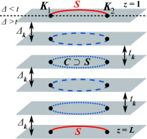
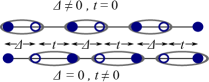
Figure 1: Above: Layering prescription for obtaining FAs of arbitrary shape. Dotted (dashed) ellipses represent electron (hole) FSs, and solid red segments are the residual FAs on adding interlayer hoppings $t_{\boldsymbol{k}}$ and $\Delta_{\boldsymbol{k}}$. The horizontal black dashed line on the topmost layer separates regions with $\Delta_{\boldsymbol{k}}>t_{\boldsymbol{k}}$ and $\Delta_{\boldsymbol{k}}<t_{\boldsymbol{k}}$. An even (odd) number of total layers gives identical (non-identical) FAs on the two surfaces, as shown on the left (right). Below: 1D systems at fixed $\boldsymbol{k}\in C$ under the influence of $\Delta$ and $t$ in the extreme cases where the smaller hopping vanishes, for even (left) and odd (right) $L$. Filled (empty) circles denote a state on an electron (a hole) Fermi surface in the limit of decoupled layers. The ellipses enclose the states which get mutually gapped out by the hoppings.

We claim that this WSM is generated by the following Bloch Hamiltonian:

$$H_{\boldsymbol{k}} = \sum_{z=1}^{L}\psi_{z,\boldsymbol{k}}^{\dagger}(-1)^{z}\mathcal{E}_{\boldsymbol{k}}\psi_{z,\boldsymbol{k}}$$

$$+\sum_{z=1}^{L-1}\psi_{z,\boldsymbol{k}}^{\dagger}h_{z,\boldsymbol{k}}\psi_{z+1,\boldsymbol{k}}+\mbox{h.c.}$$

where even (odd) $L$ generates $S=S^{\prime}$ ($S\neq S^{\prime}$), $\mathcal{E}_{\boldsymbol{k}}$ is a phenomenological function that vanishes along a contour $C$ given by

$$C\begin{cases}\supset S&S=S^{\prime}\\ =S\cup S^{\prime}&S\neq S^{\prime}\end{cases}$$ (2)

and the interlayer coupling $h_{z,\boldsymbol{k}}=-t_{\boldsymbol{k}}(\Delta_{\boldsymbol{k}})$ if $z$ is even (odd). If $S=S^{\prime}$, $C$ can be chosen arbitrarily as long as it contains the entire segment $S$. The functions $t_{\boldsymbol{k}}$ and $\Delta_{\boldsymbol{k}}$ are real, non-negative phenomenological functions that satisfy:

$$t_{\boldsymbol{k}}\begin{cases}>\Delta_{\boldsymbol{k}}&\boldsymbol{k}\in S\\ <\Delta_{\boldsymbol{k}}&\boldsymbol{k}\in C/S(=S^{\prime}\mbox{ if }C=S\cup S^{\prime})\end{cases}$$ (3)

(3) dictates that $t_{\boldsymbol{k}}=\Delta_{\boldsymbol{k}}$ exactly at $\boldsymbol{k}=\boldsymbol{K}_{1,2}$. The $\boldsymbol{k}$-dependence of $t$ and $\Delta$ away from $C$ is unimportant for our purposes, and will be assumed to be negligible henceforth. We now justify the above claim.

Bulk: If the interlayer couplings $t_{\boldsymbol{k}}=\Delta_{\boldsymbol{k}}=0$, then $\mathbb{H}=\sum_{\boldsymbol{k}}H_{\boldsymbol{k}}$ describes a stack of alternate non-degenerate electron and hole FSs. When $t_{\boldsymbol{k}}$ and $\Delta_{\boldsymbol{k}}$ are turned on, these FSs get gapped out in pairs in the bulk. Indeed, the bulk Hamiltonian is

$$H_{\boldsymbol{k},k_{z}}^{\mbox{bulk}}=\mathcal{E}_{\boldsymbol{k}}\sigma_{z}+\left(\Delta_{\boldsymbol{k}}-t_{\boldsymbol{k}}\cos k_{z}\right)\sigma_{x}+t_{\boldsymbol{k}}\sin k_{z}\sigma_{y}$$ (4)

where $z$ is the layering direction, and is gapped everywhere except at the desired Weyl points: $(\boldsymbol{k},k_{z})=\left(\boldsymbol{K}_{1,2},0\right)$, due to (3). Allowing $t_{\boldsymbol{k}}$ and $\Delta_{\boldsymbol{k}}$ to be negative or complex simply moves the Weyl points off the $k_{z}=0$ plane, but this does not affect the shape of the FAs. Near the gapless points, $H^{\mbox{bulk}}$ realizes the Weyl Hamiltonian:

$$H_{\boldsymbol{K}_{i}+\boldsymbol{p},0+p_{z}}^{\mbox{bulk}}$$

$$\,\,\,\approx\left[\boldsymbol{p}\cdotp\boldsymbol{\nabla_{k}}\mathcal{E}_{\boldsymbol{K}_{i}}\right]\sigma_{z}+\left[\boldsymbol{p}\cdot\boldsymbol{\nabla_{k}}\left(\Delta_{\boldsymbol{K}_{i}}-t_{\boldsymbol{K}_{i}}\right)\right]\sigma_{x}+\left[t_{\boldsymbol{K}_{i}}p_{z}\right]\sigma_{y}$$

$$\,\,\,\equiv p_{\perp}v_{F}(\boldsymbol{K}_{i})\sigma_{z}+p_{\parallel}v_{i}\sigma_{x}+\Delta_{0}p_{z}\sigma_{y}$$ (5)

where $p_{\perp}=\boldsymbol{p}\cdot\hat{\boldsymbol{e}}_{r}(\boldsymbol{K}_{i})$ and $p_{\parallel}=\boldsymbol{p}\cdot\hat{\boldsymbol{e}}_{t}(\boldsymbol{K}_{i})$ are momenta perpendicular and parallel to $C$ ($\hat{e}_{r}(\boldsymbol{k})$ and $\hat{\boldsymbol{e}}_{t}(\boldsymbol{k})$ are 2D unit vectors normal and tangential to $C$), $v_{F}$ is the Fermi velocity of the 2D FSs and $v_{i}=\boldsymbol{\nabla_{k}}\left(\Delta_{\boldsymbol{K}_{i}}-t_{\boldsymbol{K}_{i}}\right)\cdot\hat{e_{t}}(\boldsymbol{K}_{i})$. In going to the second line, the variation of $t_{\boldsymbol{k}}$ and $\Delta_{\boldsymbol{k}}$ perpendicular to $C$ has been assumed to be negligible, since it does not affect the shape of the FAs. $v_{i}$ has opposite signs at $\boldsymbol{K}_{1}$ and $\boldsymbol{K}_{2}$, ensuring that the Weyl nodes have opposite chirality. $H_{\mbox{bulk}}$ is obviously unaffected by the boundary conditions at $z=1$ and $z=L$ for large $L$.

Surface: The surface, however, strongly depends on the boundary conditions; in particular, it is qualitatively different for odd and even $L$. If $L$ is odd, at each $\boldsymbol{k}\in C$, a state remains unpaired and hence, gapless, at $z=1$ ($z=L$) whenever $\Delta_{\boldsymbol{k}}<t_{\boldsymbol{k}}$ ($\Delta_{\boldsymbol{k}}>t_{\boldsymbol{k}}$). The gapless states at $z=1$ ($z=L$) thus, trace out $S$ ($S^{\prime}$). On the other hand, when $L$ is even, both ends of a the chain at fixed $\boldsymbol{k}$ carry a gapless state when $\Delta_{\boldsymbol{k}}<t_{\boldsymbol{k}}$ and neither end has gapless states when $\Delta_{\boldsymbol{k}}>t_{\boldsymbol{k}}$. In this case, the gapless states on both surfaces of the slab trace out $S$.

Viewed differently, the 1D system at fixed $\boldsymbol{k}\in C$ and $\left|\Delta\right|\neq\left|t\right|$ is an insulator in the CII symmetry class, which is known to have a $\mathbb{Z}$ topological classification Schnyder et al. (2008); Kitaev (2009). While $\left|\Delta\right|>\left|t\right|$ gives a trivial phase, $\left|\Delta\right|<\left|t\right|$ is topologically non-trivial with a zero mode at each end protected by a chiral symmetry, if the 1D lattice has a whole number of unit cells. These end states are nothing but the FA states at that $\boldsymbol{k}$ when $L$ is even. As $\boldsymbol{k}$ is varied along $C$, the 1D system undergoes a topological phase transition at $\boldsymbol{K}_{1}$ and $\boldsymbol{K}_{2}$. For odd $L$, there is always a state at one end of the chain, as show in Fig 1. This prescription is similar in spirit to node-pairing picture of Ref Hosur et al. (2010) for chiral topological insulators in three dimensions. Note that it is necessary to start with two sets of FSs, since a single FS cannot be destroyed perturbatively.

Symmetry analysis: WSMs can only exist in systems in which at least one symmetry out of time-reversal symmetry ($\mathcal{T}$) and inversion symmetry ($\mathcal{I}$) is broken; the presence of both would make each band doubly degenerate and give Dirac semi-metals instead with four-component fermions near at each node. Moreover, $\mathcal{I}$-symmetric, $\mathcal{T}$-breaking ($\mathcal{T}$-symmetric, $\mathcal{I}$-breaking) WSMs have an odd (even) number of pairs of Weyl nodes. In the current picture, the breaking of these symmetries can be understood as follows. Let us assume $\mathcal{E}_{\boldsymbol{k}}=\mathcal{E}_{-\boldsymbol{k}}$; if this weren’t true, both symmetries would broken from the outset. In general, $t_{\boldsymbol{k}}$ and $\Delta_{\boldsymbol{k}}$ are unrelated to $t_{-\boldsymbol{k}}$ and $\Delta_{-\boldsymbol{k}}$, in which case both symmetries would again be broken. However, $\mathcal{T}$ is preserved if $t_{\boldsymbol{k}}=t_{-\boldsymbol{k}}$ and $\Delta_{\boldsymbol{k}}=\Delta_{-\boldsymbol{k}}$, which can only happen if the number of points on $C$ at which $t_{\boldsymbol{k}}=\Delta_{\boldsymbol{k}}$, and thus the number of Weyl nodes, is an integer multiple of four. On the other hand, inversion about a particular layer interchanges $t$ and $\Delta$; thus, $t_{\boldsymbol{k}}=\Delta_{-\boldsymbol{k}}$ preserves this inversion symmetry. This condition requires $t_{\boldsymbol{k}}-\Delta_{\boldsymbol{k}}$ to change sign twice an odd number of times along $C$, giving an odd number of Weyl node pairs.

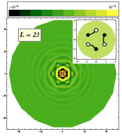
(a)                              (b)                                            (c)

Figure 2: (a) FAs in the surface Brillouin zone on the 111 surface of iridate WSMs. Solid (dashed) lines denote FAs on the near (far) surface. Filled (empty) circles denote projections of Weyl nodes of positive (negative) chirality in all the figures above. (b and c) Surface LDOS in arbitrary units due to the six FAs near the $L$ point in the presence of a point scatterer on the surface (brown cross) for a thin sample (b) and a thick sample (c). Insets show the numerically computed surface spectral function at $E=0$ for the clean system, with darker colors representing larger values. The computation is done for the model, described in the text, which generates the six FAs near the $L$-point but not the remaining eighteen FAs near the Brillouin zone edges.

LDOS results: Having described the procedure for obtaining FAs from a 2D limit, we demonstrate its utility by calculating the surface spectral function for a clean system and the surface LDOS in the presence of a point surface scatterer within a model that should be relevant to the pyrochlore iridates A₂Ir₂O₇, A$=$Y, Eu, which are purported WSMs with 24 Weyl nodes Wan et al. (2011). The lattice in the WSM phase has inversion symmetry as well as a threefold rotation symmetry $R_{3}$ about the cubic 111-axis, and there are six Weyl nodes related by these symmetries near each of the four $L$ points in the FCC Brillouin zone. Additionally, the lattice also has a $D_{6}$ symmetry, i.e., $\pi/3$ rotation about [111] followed by reflection in the perpendicular plane. This symmetry has an important implication for the FAs: if it is preserved in a slab geometry, then the FAs will be as shown in Fig 2 (a). In particular, the six FAs near the center of the surface Brillouin zone enclose an area, while the remaining eighteen overlap in pairs on the opposite surfaces. We note that Ref Witczak-Krempa and Kim (2012) also predicted Weyl semimetallic behavior in the above iridates, but with only 8 Weyl nodes. In this case, the hexagonal figure around the $L$ point would collapse to a point. As we argue below, LDOS oscillations on the surface stem predominantly from the hexagonal figure; hence, the proposal of Ref Witczak-Krempa and Kim (2012), if true, would imply no strong LDOS oscillations.

We compute the surface LDOS for a model that has six FAs like the ones around the $L$ point, as a function of the the sample thickness. The remaining eighteen FAs in the iridates are expected to be destroyed by finite size effects for thin samples, while for thick samples backscattering occurs across the Brillouin zone and hence can give rise to LDOS oscillations only on the lattice scale. These oscillations are unlikely to be distinguishable from the electron density variations on this scale already present.

The LDOS is calculated via the standard $T$-matrix formalism. Given the time-ordered Green’s function for the clean system: $G_{0}(\boldsymbol{k},E)=\left(E-H_{\boldsymbol{k}}\right)^{-1}$ and a scattering potential: $U_{z,z^{\prime}}(x,y)=u\delta(x)\delta(y)\delta_{z,1}\delta_{z^{\prime},1}$, the $T$-matrix is given by $T(\omega)=\left(1-U\sum_{\boldsymbol{k}}G_{0}(\boldsymbol{k},E)\right)^{-1}U$, independent of momentum, since the scattering potential in momentum independent. Here, $G_{0}$, $U$ and $T$ are all $L\times L$ matrices indexed by $z$. The full Green’s function in the presence of the impurity is $G(\boldsymbol{k},\boldsymbol{k}^{\prime},E)=\delta_{\boldsymbol{k},\boldsymbol{k}^{\prime}}G_{0}(\boldsymbol{k},E)+G_{0}(\boldsymbol{k},E)T(\omega)G_{0}(\boldsymbol{k}^{\prime},E)$, and the LDOS on the $z=1$ surface is related to the $(1,1)$ element of its retarded cousin: $\rho_{\mbox{surf}}(\boldsymbol{r},E)=-\frac{1}{\pi}\mathrm{Im}G^{11}(\boldsymbol{r},\boldsymbol{r},E+i\delta)$, where $G(\boldsymbol{r},\boldsymbol{r}^{\prime},E)=\int_{\boldsymbol{k},\boldsymbol{k}^{\prime}}e^{i(\boldsymbol{k}\cdot\boldsymbol{r}-\boldsymbol{k}^{\prime}\cdot\boldsymbol{r}^{\prime})}G(\boldsymbol{k},\boldsymbol{k}^{\prime},E)$. For the calculation, we use $\mathcal{E}(\boldsymbol{k})=\sqrt{k^{2}+2k^{6}\cos^{2}3\theta_{\boldsymbol{k}}}-1$ to generate the hexagonal figure and $t_{\boldsymbol{k}}\equiv t_{0}=0.5$, $\Delta_{\boldsymbol{k}}=t_{0}(1-\cos 3\theta_{\boldsymbol{k}})$ to obtain the FAs. Here, $(k,\theta_{\boldsymbol{k}})$ the polar coordinates of $\boldsymbol{k}$.

The results are presented in Fig 2 (b) and (c) for $E=0$. For thin samples, clear LDOS oscillations are seen in the horizontal direction as well as along the two equivalent directions related by $\pi/3$ rotation. The origin of these oscillations becomes clear if one looks at $A_{\mbox{surf}}^{0}(\boldsymbol{k},E=0)$, displayed inset. Since the sample is thin, FA wavefunctions from the far surface have significant amplitude on the near surface, which allows backscattering to occur diametrically across the hexagon. The dominant backscattering processes are the ones involving the midpoints of the FAs, since the Fermi surface is nested here. On the other hand, as the sample thickness is increased, three of the six FAs retreat to the far surface and backscattering is exponentially suppressed. The result is small variations in the LDOS arising from scattering between FAs solely on the top surface. Thus, the STM map has a distinct evolution with sample thickness which is characteristic of the FA structure in the iridate WSMs.

Surface spectral function in clean thermodynamic limit: $A_{\mbox{surf}}^{0}(\boldsymbol{k},E)$ was computed numerically in order to generate the insets of Fig 2. In the thermodynamic limit, however, this calculation can be done analytically. Denoting the $(1,1)$ element of the clean Green’s function for a $L$-layer slab by $G_{0(L)}^{11}$, it is straightforward to show, by explicitly evaluating the $(1,1)$ cofactor of $E-H_{\boldsymbol{k}}$ and using $\mathrm{det}\left(\begin{array}[]{cc}A&B\\ C&D\end{array}\right)=\mathrm{det}(A)\mathrm{det}(D-CA^{-1}B)$, that

$$(E-\mathcal{E}_{\boldsymbol{k}})G_{0(L)}^{11}(\boldsymbol{k},E)$$

$$=1+\frac{\Delta_{\boldsymbol{k}}^{2}}{E^{2}-\mathcal{E}_{\boldsymbol{k}}^{2}-\Delta_{\boldsymbol{k}}^{2}-t_{\boldsymbol{k}}^{2}(E-\mathcal{E}_{\boldsymbol{k}})G_{0(L-2)}^{11}(\boldsymbol{k},E)}$$ (6)

In the thermodynamic limit: $L\to\infty$, $G_{0(L)}^{11}(\boldsymbol{k},E)\approx G_{0(L-2)}^{11}(\boldsymbol{k},E)\equiv g(\boldsymbol{k},E)$. Thus,

$$g(\boldsymbol{k},E)=\frac{1}{2t_{\boldsymbol{k}}^{2}(E-\mathcal{E}_{\boldsymbol{k}})}\left[\left(E^{2}-\mathcal{E}_{\boldsymbol{k}}^{2}+t_{\boldsymbol{k}}^{2}-\Delta_{\boldsymbol{k}}^{2}\right)\pm\sqrt{\left(E^{2}-\mathcal{E}_{\boldsymbol{k}}^{2}+t_{\boldsymbol{k}}^{2}-\Delta_{\boldsymbol{k}}^{2}\right)^{2}-4t_{\boldsymbol{k}}^{2}(E^{2}-\mathcal{E}_{\boldsymbol{k}}^{2})}\right]$$ (7)

The physical condition $A_{\mbox{surf}}^{0}(\boldsymbol{k},E)=-\frac{1}{\pi}\mathrm{Im}\left[g(\boldsymbol{k},E+i\delta)\right]\geq 0$ fixes the sign in front of the square root. Clearly,

$$A_{\mbox{surf}}^{0}(\boldsymbol{k},E)=\delta(E-\mathcal{E}_{\boldsymbol{k}})\frac{t_{\boldsymbol{k}}^{2}-\Delta_{\boldsymbol{k}}^{2}+\left|t_{\boldsymbol{k}}^{2}-\Delta_{\boldsymbol{k}}^{2}\right|}{2t_{\boldsymbol{k}}^{2}}+$$

$$\frac{1}{2t_{\boldsymbol{k}}^{2}(E-\mathcal{E}_{\boldsymbol{k}})}\mathrm{Im}\sqrt{\left(E^{2}-\mathcal{E}_{\boldsymbol{k}}^{2}+t_{\boldsymbol{k}}^{2}-\Delta_{\boldsymbol{k}}^{2}\right)^{2}-4t_{\boldsymbol{k}}^{2}(E^{2}-\mathcal{E}_{\boldsymbol{k}}^{2})}$$ (8)

The first line is non-zero only when $t_{\boldsymbol{k}}^{2}>\Delta_{\boldsymbol{k}}^{2}$ and has a sharp peak at $E=\mathcal{E}_{\boldsymbol{k}}$. Clearly, this represents the contribution to $A_{\mbox{surf}}^{0}$ from the FA. Whereas, the second line is non-vanishing when $|E|>|\mathcal{E}_{\boldsymbol{k}}|$ and $\left|t_{\boldsymbol{k}}-\sqrt{E^{2}-\mathcal{E}_{\boldsymbol{k}}^{2}}\right|<|\Delta_{\boldsymbol{k}}|<\left|t_{\boldsymbol{k}}+\sqrt{E^{2}-\mathcal{E}_{\boldsymbol{k}}^{2}}\right|$. These inequalities are satisfied in the region near the projection of the Weyl points onto the surface. Moreover, this contribution to $A_{\mbox{surf}}^{0}$ has no delta-function peak. Thus, it represents contributions form the bulk states near the Weyl nodes. The quantity $A_{\mbox{surf}}^{0}$ can be directly measured by ARPES experiments.

In conclusion, we have studied impurity-induced Friedel oscillations due to FAs in WSMs, focusing on the FA structure of the purported iridate WSMs, and observed their dependence on sample thickness. For thin samples, FAs on both surfaces collude to allow nested backscattering and hence produce strong LDOS oscillations, whereas for thick samples, the FAs on the far surface do not reach the near surface and such backscattering and the consequent LDOS oscillations are suppressed. The calculation is done by building the desired WSM and FA structure by stacking electron and hole Fermi surfaces and adding suitable interlayer hopping. Within this prescription, the surface spectral function for a clean system can be calculated analytically in the thermodynamic limit.