Probing dark radiation with inflationary gravitational waves

Abstract

Recent cosmological observations indicate the existence of extra light species, i.e., dark radiation. In this paper we show that signatures of the dark radiation are imprinted in the spectrum of inflationary gravitational waves. If the dark radiation is produced by the decay of a massive particle, high frequency mode of the gravitational waves are suppressed. In addition, due to the effect of the anisotropic stress caused by the dark radiation, a dip in the gravitational wave spectrum may show up at the frequency which enters the horizon at the time of the dark radiation production. Once the gravitational wave spectrum is experimentally studied in detail, we can infer the information on how and when the dark radiation was produced in the Universe.

I Introduction

Recently, there are increasing evidence of the extra non-interacting relativistic degrees of freedom, in addition to the standard three (nearly) massless neutrino species. The abundance of relativistic component is parametrized by the effective number of neutrino species, $N_{\rm eff}$, as

$$\rho_{\rm rel}=\left[1+N_{\rm eff}\frac{7}{8}\left(\frac{4}{11}\right)^{4/3}\right]\rho_{\gamma},$$ (1)

where $\rho_{\rm rel}$ is the total relativistic energy density and $\rho_{\gamma}=(\pi^{2}/15)T_{\gamma}^{4}$ denotes the photon energy density measured after the $e^{+}e^{-}$ annihilation with $T_{\gamma}$ representing the photon temperature. The standard model predicts $N_{\rm eff}=3.05$ Mangano:2005cc .

The $N_{\rm eff}$ can be constrained from various observations. First, increasing $N_{\rm eff}$ leads to larger Hubble expansion rate at the big bang nucleosynthesis epoch, which in turn results in increase of the primordial helium abundance. Recent observations suggest $N_{\rm eff}=3.68^{+0.80}_{-0.70}$ at $2\sigma$ level Izotov:2010ca . (See, however, also Ref. Aver:2010wq for discussion on the error estimation in the helium abundance.)

The cosmic microwave background (CMB) anisotropy is also sensitive to $N_{\rm eff}$. The information on $N_{\rm eff}$ is imprinted in the CMB anisotropy in some ways. First, increase of $N_{\rm eff}$ makes the early integrated Sachs-Wolfe effect more efficient, and the first peak of the CMB power spectrum is enhanced. Second, it tends to make the scale of sound horizon smaller at the recombination epoch, resulting in shift of the peak positions in the CMB power spectrum toward high multipole moment. Third, it erases the small scale power spectrum due to the effect of free-streaming. The WMAP seven-year results combined with standard rulers give $N_{\rm eff}=4.32^{+0.86}_{-0.88}$ at $1\sigma$ level Komatsu:2010fb . Adding small scale CMB measurements improves the accuracy as $N_{\rm eff}=4.56\pm 0.75$ for ACT Dunkley:2010ge and $N_{\rm eff}=3.86\pm 0.42$ for SPT Keisler:2011aw both at $1\sigma$ level. Ref. Archidiacono:2011gq combined the WMAP, ACT and SPT datasets with standard rulers and obtained $N_{\rm eff}=4.08^{+0.71}_{-0.68}$ at $2\sigma$ level. See also recent related studies Hamann:2011hu ; Nollett:2011aa ; Hamann:2010bk ; Hamann:2011ge .

To summarize, at the current situation, observations suggest $\Delta N_{\rm eff}\equiv N_{\rm eff}-3\simeq 1$ at nearly $2\sigma$ level. Motivated by these increasing evidence of the extra light species, which is often called “dark radiation”, models to explain dark radiation were proposed Ichikawa:2007jv ; Jaeckel:2008fi ; Nakayama:2010vs ; Fischler:2010xz ; Kawasaki:2011ym ; Hall:2011zq ; Hasenkamp:2011em ; Kawasaki:2011rc ; Menestrina:2011mz ; Kobayashi:2011hp ; Hooper:2011aj ; Jeong:2012hp ; Kawakami:2012ke ; Blennow:2012de ; Moroi:2012vu . Although there are many candidates, if the dark radiation has only extremely weak interaction with the standard model particles, it may be difficult to detect it experimentally. Thus it is important to study how to confirm and distinguish models of dark radiation by other observations. For example, in Refs. Kawasaki:2011rc ; Kawakami:2012ke the possibility that the dark radiation has (non-Gaussian) isocurvature perturbations was considered. In Ref. Zhao:2009aj the effect of dark radiation on CMB B-mode spectrum is discussed.

In this paper we consider a novel method to detect dark radiation through inflationary gravitational waves (GWs). It is known that relativistic free streaming fluid can contribute to the anisotropic stress, which potentially affects the propagation of GWs Weinberg:2003ur . This effect was concretely studied for the free-streaming neutrinos. GWs entering the horizon after the neutrino freezeout dissipate their energies and, as a result, a modulation feature shows up in the GW spectrum Weinberg:2003ur ; Dicus:2005rh ; Watanabe:2006qe . It was also studied in the context of large lepton asymmetry Ichiki:2006rn . Therefore, it is expected that the dark radiation also induces similar effects on GWs. As opposed to the case of neutrinos, we do not know when and how the dark radiation was generated in the Universe. Thus the position and strength of the modulation in the GWs, if detected, tells us exactly about the production mechanism of dark radiation. In particular, models of dark radiation produced by decay of non-relativistic fields Ichikawa:2007jv ; Fischler:2010xz ; Kawasaki:2011ym ; Hasenkamp:2011em ; Kawasaki:2011rc ; Menestrina:2011mz ; Kobayashi:2011hp ; Hooper:2011aj ; Jeong:2012hp shows characteristic features in the primordial GW spectrum. The feature consists of combination of the anisotropic stress effect and the modified background expansion history. This is detectable in future space-based GW detectors such as DECIGO Seto:2001qf and BBO Crowder:2005nr ; Cutler:2009qv . We also show that the GW spectrum will be a powerful tool for confirming the dark radiation produced thermally and decoupled at some epoch in the early Universe.

This paper is organized as follows. In Sec. II we review a model of dark radiation produced by decaying particles. In Sec. III we calculate the evolution of gravitational waves in the presence of anisotropic stress induced by dark radiation, and show that characteristic signatures appear in the spectrum. Sec. IV is devoted to conclusions and discussion.

II Dark radiation production by decaying particles

II.1 Background evolution

We consider the case where the non-relativistic matter $\phi$ decays into $X$ particle which plays the role of dark radiation. Thus $X$ is assumed to be massless and has no interaction with other fields. To be more precise, $X$ must be relativistic until the recombination epoch and its interaction must be so weak that remains to be decoupled from thermal bath after the production by $\phi$ decay. The evolution equations of components are given by

$$\dot{\rho}_{\phi}+3H\rho_{\phi}=-\Gamma_{\phi}\rho_{\phi},$$ (2)

$$\dot{\rho}_{\rm rad}+4H\rho_{\rm rad}=\Gamma_{\phi}(1-B_{X})\rho_{\phi},$$ (3)

$$\dot{\rho}_{X}+4H\rho_{X}=\Gamma_{\phi}B_{X}\rho_{\phi},$$ (4)

where the dot represents time derivative, and the Friedmann equation,

$$H^{2}=\frac{\rho_{\rm tot}}{3M_{P}^{2}}=\frac{\rho_{\phi}+\rho_{\rm rad}+\rho_{X}}{3M_{P}^{2}},$$ (5)

where $\rho_{\phi},\rho_{\rm rad}$ and $\rho_{X}$ are energy densities of $\phi$, visible radiation and dark radiation, respectively, $M_{P}$ is the reduced Planck scale, $\Gamma_{\phi}$ is the decay rate of $\phi$, and $B_{X}$ denotes its branching fraction into $X$.

The extra effective number of neutrino species is given by

$$\Delta N_{\rm eff}=\frac{43}{7}\left[\frac{10.75}{g_{*s}(T_{\phi})}\right]^{1/3}\left[\frac{\rho_{X}}{\rho_{\rm rad}}\right]_{H\ll\Gamma_{\phi}},$$ (6)

where $g_{*s}(T_{\phi})$ denotes the relativistic degrees of freedom at $T=T_{\phi}$ where the $\phi$ decays, and $\rho_{X}$ and $\rho_{\rm rad}$ are evaluated well after the $\phi$ decay. In our numerical study we take the standard-model value of $g_{*s}(T_{\phi})=106.75$, because as we will see, $T_{\phi}\gg T_{\rm EW}\simeq\mathcal{O}(100)\,{\rm GeV}$ is necessary for observation.

In order to obtain $\Delta N_{\rm eff}\simeq 1$, the energy density of $\phi$ should nearly dominate the Universe at the decay. Therefore, the expansion rate of the Universe around the $\phi$ decay epoch is modified. Fig. 1 shows the product $tH$ as a function of cosmic time $t$ normalized by $t_{\rm dec}$, defined by

$$t_{\rm dec}\equiv\frac{1}{\Gamma_{\phi}}.$$ (7)

Here we have fixed initial conditions of $\rho_{\phi}$ and $\rho_{\rm rad}$ so that $\Delta N_{\rm eff}=1$ is realized. Solid (red), long-dashed (green), short-dashed (blue) and dotted (magenta) lines correspond to $B_{X}=0.26$, $0.5$, $0.7$ and $1.0$, respectively. It is seen that $\phi$ has significant energy fraction around its decay and the expansion rate is modified from the radiation-dominated one ($tH=1/2$). In the limit of $\phi$ domination, we need $B_{X}\simeq 0.26$ for $\Delta N_{\rm eff}=1$. Thus $B_{X}\gtrsim 0.26$ is required in order to realize $\Delta N_{\rm eff}=1$: otherwise, the $X$ energy density would be too small to explain $\Delta N_{\rm eff}=1$ even if $\phi$ dominates the Universe. Since the background expansion rate is imprinted in the GW spectrum Turner:1990rc ; Seto:2003kc ; Tashiro:2003qp ; Boyle:2005se ; Boyle:2007zx ; Nakayama:2008ip ; Nakayama:2008wy ; Kuroyanagi:2008ye ; Mukohyama:2009zs ; Nakayama:2009ce ; Nakayama:2010kt ; Schettler:2010dp ; Durrer:2011bi ; Kuroyanagi:2011fy ; Jinno:2011sw ; Saito:2012bb , a particular shape in the GW spectrum is expected if dark radiation is produced by decaying matter, as we will see.

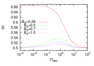
Figure 1: Evolution of the product $tH$ as a function of cosmic time (normalized by $t_{\rm dec}$) for $B_{X}=0.26$ (red solid), $0.5$ (green dashed), $0.7$ (blue dotted) and $1.0$ (magenta dot-dashed) for explaining $\Delta N_{\rm eff}=1$.

II.2 Model

As one of the motivated models of $\phi$ and $X$, we consider the saxion and axion in a supersymmetric axion model Rajagopal:1990yx . This possibility was studied in Refs. Ichikawa:2007jv ; Kawasaki:2011ym ; Kawasaki:2011rc ; Jeong:2012hp ; Moroi:2012vu in the context of dark radiation.

The axion is a pseudo Nambu-Goldstone boson associated with the spontaneous breakdown of the global U(1)_PQ symmetry Peccei:1977hh . It solves the strong CP problem in the quantum chromodynamics. The axion has interactions suppressed by the U(1)_PQ breaking scale, $f_{a}$. The value of $f_{a}$ is phenomenologically constrained as $10^{9}$ GeV $\lesssim f_{a}\lesssim 10^{12}$ GeV, and the axion mass is $\sim 10^{-2}$–$10^{-5}$ eV for this range of $f_{a}$ Kim:1986ax . Thus the axion is a good candidate of dark radiation.

In a supersymmetric extension of the axion model, there appears a scalar partner of the axion, called saxion, which is massless in supersymmetric limit but obtains a mass from supersymmetry breaking effects. Writing the saxion mass as $m_{\phi}$, the saxion decay rate into the axion pair is given by Chun:1995hc

$$\Gamma_{\phi}=\frac{\xi^{2}}{64\pi}\frac{m_{\phi}^{3}}{f_{a}^{2}}.$$ (8)

where $\xi$ is a model-dependent constant of order unity. Assuming that the saxion decays in the radiation dominated era in order to make the signal detectable, the temperature at the saxion decay is estimated to be

$$T_{\phi}\sim 3\times 10^{6}\,{\rm GeV}\left(\frac{m_{\phi}}{10^{3}\,{\rm TeV}}\right)^{3/2}\left(\frac{10^{10}\,{\rm GeV}}{f_{a}}\right).$$ (9)

The saxion with mass of $\mathcal{O}(10^{3})\,{\rm TeV}$ is plausible by taking account of the preference for high-supersymmetry breaking scale Giudice:2011cg in light of the recent discovery of the Higgs boson mass of 125 GeV Higgs . The saxion often dominantly decays into the axion pair $(B_{X}\simeq 1)$. The produced axions are never thermalized below the temperature $\sim 10^{7}$ GeV for $f_{a}\gtrsim 10^{10}$ GeV Graf:2010tv . Assuming that the saxion begins a coherent oscilation at $H=m_{\phi}$ with initial amplitude of $\phi_{i}$, the saxion abundance in terms of the energy-to-entropy ratio is given by $\rho_{\phi}/s\sim T_{\rm R}(\phi_{i}/M_{P})^{2}$, where $T_{\rm R}$ is the reheating temperature after inflation. Then the abundance of relativistic axion after the $\phi$ decay is estimated to be

$$\left[\frac{\rho_{X}}{\rho_{\rm rad}}\right]_{H\ll\Gamma_{\phi}}\sim B_{X}\left[\frac{\rho_{\phi}}{\rho_{\rm tot}}\right]_{H=\Gamma_{\phi}}\simeq\frac{B_{X}}{6}\frac{T_{\rm R}}{T_{\phi}}\left(\frac{\phi_{i}}{M_{P}}\right)^{2}.$$ (10)

Therefore, for appropriate choices of $T_{\rm R}$ and $\phi_{i}$, e.g., for $T_{\rm R}\sim T_{\phi}$ and $\phi_{i}\sim M_{P}$, the axion abundance produced by the saxion decay can account for the dark radiation : $\Delta N_{\rm eff}\simeq 1$ (see Eq. (6)).

III Spectrum of gravitational wave background with dark radiation

III.1 Evolution equations

Now let us study the evolution of primordial GWs under the presence of dark radiation. The GW corresponds to the tensor perturbation of the metric. We define the line element as

$$ds^{2}=-dt^{2}+a^{2}(t)(\delta_{ij}+h_{ij})dx^{i}dx^{j},$$ (11)

where $h_{ij}$ is the transverse and traceless part of the metric perturbation, and the Fourier amplitude of $h_{ij}$ as

$$\begin{split}h_{ij}(t,\mathbf{x})&=\int\frac{d^{3}k}{(2\pi)^{3}}h_{ij}(t,\mathbf{k})e^{i\mathbf{k}\mathbf{x}}\\ &=\sum_{\lambda=+,\times}\int\frac{d^{3}k}{(2\pi)^{3}}h^{(\lambda)}(t,\mathbf{k})\epsilon_{ij}^{(\lambda)}e^{i\mathbf{k}\mathbf{x}},\end{split}$$ (12)

where $\epsilon_{ij}^{(\lambda)}$ denotes the polarization tensor. As shown in Appendix, $h^{(\lambda)}(t,\mathbf{k})$ satisfies the following equation

$$\begin{split}\ddot{h}^{(\lambda)}&(t,\mathbf{k})+3H\dot{h}^{(\lambda)}(t,\mathbf{k})+\frac{k^{2}}{a^{2}}h^{(\lambda)}(t,\mathbf{k})\\ =&-24H^{2}\frac{1}{a^{4}(t)\rho_{\rm tot}(t)}\\ &\times\int_{0}^{t}a^{4}(t^{\prime})\rho_{X}(t^{\prime})K\left(k\int_{t^{\prime}}^{t}\frac{dt^{\prime\prime}}{a(t^{\prime\prime})}\right)\dot{h}^{(\lambda)}(t^{\prime},\mathbf{k})dt^{\prime},\\ \end{split}$$ (13)

where

$$K(u)\equiv\frac{j_{2}(u)}{u^{2}}=-\frac{\sin(u)}{u^{3}}-\frac{3\cos(u)}{u^{4}}+\frac{3\sin(u)}{u^{5}},$$ (14)

with $j_{2}$ being the second-order spherical Bessel function. Here we have assumed that there is no source for the anisotropic stress except for that induced by GW effects on dark radiation. Contrary to the case of neutrinos studied in Refs. Weinberg:2003ur ; Watanabe:2006qe , $\rho_{X}(t^{\prime})$ is inside the time integral since $\rho_{X}$ does not scale as $a^{-4}$ while $X$ is produced by the $\phi$ decay. In terms of $u$ and $u^{\prime}$ defined as

$$u = k\eta=k\int_{0}^{t}\frac{dt^{\prime}}{a(t^{\prime})},$$ (15)

$$u^{\prime} = k\eta^{\prime}=k\int_{0}^{t^{\prime}}\frac{dt^{\prime\prime}}{a(t^{\prime\prime})},$$ (16)

where $\eta\equiv\int_{0}^{t}\frac{dt^{\prime}}{a(t^{\prime})}$ is the conformal time, Eq. (LABEL:eq_hdif_t) becomes

$$\begin{split}\frac{\partial^{2}h^{(\lambda)}}{\partial u^{2}}&(u,\mathbf{k})+2H_{u}\frac{\partial h^{(\lambda)}}{\partial u}(u,\mathbf{k})+h^{(\lambda)}(u,\mathbf{k})\\ =&-24H_{u}^{2}\frac{1}{a^{4}(u)\rho_{\rm tot}(u)}\\ &\times\int_{0}^{u}a^{4}(u^{\prime})\rho_{X}(u^{\prime})K(u-u^{\prime})\frac{\partial h^{(\lambda)}}{\partial u}(u^{\prime},\mathbf{k})du^{\prime},\end{split}$$ (17)

with $H_{u}\equiv\frac{1}{a}\frac{\partial a}{\partial u}$. The RHS of Eq. (17) have effects mainly for $u\sim 1$, which roughly equals to the time of horizon-crossing, $k=aH$.

We have solved Eq. (17) together with the background evolution (2) – (4) to derive the present GW spectrum.

III.2 Overall normalization

Before showing the detailed results, we here comment on the normalization of the present GW energy density. During inflation, quantum fluctuations of the tensor perturbation is continuously generated which turn into stochastic GW background in the present Universe after the horizon-in Maggiore:1999vm . It predicts nearly scale invariant GW spectrum for the GW modes entering in the horizon in the radiation-dominated era Allen:1987bk ; Sahni:1990tx ; Turner:1993vb ; Turner:1996ck ; Smith:2005mm ; Smith:2006xf ; Chongchitnan:2006pe ; Friedman:2006zt . The GW energy density per log frequency at the horizon crossing $k=aH$, normalized by the critical energy density, is given by Smith:2008pf

$$\Omega_{\rm GW}(k=aH)=\frac{\Delta_{h}^{2}(k)}{24}\simeq\frac{2.43\times 10^{-9}r}{24}\left(\frac{k}{k_{0}}\right)^{n_{t}},$$ (18)

where $r$ denotes the tensor-to-scalar ratio, $n_{t}$ is the tensor spectral index, $k_{0}=0.002\,{\rm Mpc^{-1}}$ is the pivot scale and

$$\Delta_{h}^{2}(k)\equiv\frac{8}{M_{P}^{2}}\left(\frac{H_{\rm inf}}{2\pi}\right)^{2}\left(\frac{k}{k_{0}}\right)^{n_{t}},$$ (19)

with $H_{\rm inf}$ being the Hubble scale during inflation and we have assumed the WMAP normalization on the curvature perturbation on large scale Komatsu:2010fb . In this subsection, we consider the modes which enter the horizon in the radiation-dominated era, since we are interested in the high-frequency GWs which may be observed by space-based GW detectors.

First, in the standard model without dark radiation, the present spectrum of GWs is given by

$$\Omega_{\rm GW}^{\rm(SM)}(k)=\gamma^{\rm(SM)}\Omega_{\rm rad}^{\rm(SM)}\times\Omega_{\rm GW}(k=aH),$$ (20)

where $\Omega_{\rm rad}^{\rm(SM)}=4.2\times 10^{-5}h^{-2}$ with $h$ parameterizing the present Hubble parameter as $H_{0}=100h$ km/s/Mpc and

$$\gamma^{\rm(SM)}=\left[\frac{g_{*}(T_{\rm in}(k))}{g_{*0}^{\rm(SM)}}\right]\left[\frac{g_{*s0}^{\rm(SM)}}{g_{*s}(T_{\rm in}(k))}\right]^{4/3},$$ (21)

where $g_{*0}^{\rm(SM)}=3.36$ and $g_{*s0}^{\rm(SM)}=3.91$, and $T_{\rm in}(k)$ denotes the temperature at which the mode $k$ enters the horizon. Eq. (20) reflects the fact that GWs behave as a relativistic component after they have entered the horizon. We have $\gamma^{\rm(SM)}\simeq 0.39$ for $g_{*}(T_{\rm in}(k))=106.75$. The present GW spectrum per log frequency is then given by

$$\Omega_{\rm GW}^{\rm(SM)}(k) \simeq 3.3\times 10^{-16}$$ (22)

$$\times\left(\frac{r}{0.1}\right)\left(\frac{k}{k_{0}}\right)^{n_{t}}\left[\frac{106.75}{g_{*}(T_{\rm in}(k))}\right]^{1/3}.$$

In the presence of dark radiation, the overall normalization of the GW spectrum is modified due to the change of expansion rate. Neglecting the effect of anisotropic stress, we find

$$\Omega_{\rm GW}(k)=\gamma\Omega_{\rm rad}\times\Omega_{\rm GW}(k=aH),$$ (23)

where $\Omega_{\rm rad}=\Omega_{\rm rad}^{\rm(SM)}\times(g_{*0}/g_{*0}^{\rm(SM)})$ with

$$g_{*0}=2\left[1+N_{\rm eff}\frac{7}{8}\left(\frac{4}{11}\right)^{4/3}\right].$$ (24)

We find $g_{*0}\simeq 3.82$ for $N_{\rm eff}=4$. The factor $\gamma$ is given by

$$\gamma=\frac{1+\frac{7}{43}\left(\frac{g_{*s}(T_{\phi})}{10.75}\right)^{1/3}\Delta N_{\rm eff}}{1/\gamma^{\rm(SM)}+\frac{7}{43}\left(\frac{g_{*s}(T_{\phi})}{10.75}\right)^{1/3}\Delta N_{\rm eff}},$$ (25)

where we have used the relation (6). Therefore, the overall enhancement factor for the GW spectrum is given by

$$C_{1}\equiv\frac{\gamma}{\gamma^{\rm(SM)}}\frac{g_{*0}}{g_{*0}^{\rm(SM)}},$$ (26)

which is $1.35$ for $\Delta N_{\rm eff}=1$. The first factor comes from the modified expansion rate between the horizon-in and matter-radiation equality, and the second factor comes from the change of the epoch of matter-radiation equality. Thus, without the effect of anisotropic stress, the GW amplitudes at high frequencies inferred from the measured tensor-to-scalar ratio at the CMB scales are enhanced in the presence of dark radiation.

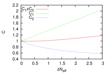
Figure 2: Relative normalization of the GW spectrum for $k_{\rm EW}\ll k\ll k_{\rm dec}$ as a function of $\Delta N_{\rm eff}$. $C_{1}$ (green dashed) : the enhancement factor due to the modified background evolution. $C_{2}$ (blue dotted) : the suppression factor due to the anisotropic stress caused by dark radiation. Their product $C_{1}\times C_{2}$ (red solid) determines the resulting overall normalization for the modes $k_{\rm EW}\ll k\ll k_{\rm dec}$.

Such an enhancement is compensated by the dissipation of GWs caused by the anisotropic stress of dark radiation. The suppression factor due to the anisotropic stress, which we express here by $C_{2}$, was analytically derived in Ref. Dicus:2005rh ; Boyle:2005se as a function of energy fraction of relativistic free-streaming particles with respect to the total radiation energy density, which was assumed to be constant around the time of horizon-crossing. Thus we can apply their result to the present situation only for $k\ll k_{\rm dec}$, where $k_{\rm dec}$ denotes the comoving Hubble scale at $t=t_{\rm dec}$ :

$$k_{\rm dec}\equiv a(t_{\rm dec})H(t_{\rm dec}),$$ (27)

because $\phi$ has completely decayed and the energy fraction of $X$ is constant after the horizon crossing for the mode $k\ll k_{\rm dec}$. In terms of $T_{\phi}$, it is given by

$$k_{\rm dec}\simeq 0.27\,{\rm Hz}\left(\frac{T_{\phi}}{10^{7}\,{\rm GeV}}\right)\left(\frac{g_{*s}(T_{\phi})}{106.75}\right)^{1/6}.$$ (28)

If it is around $\mathcal{O}(1)$ Hz, the GW features around $k\sim k_{\rm dec}$ is observable at DECIGO/BBO Seto:2001qf ; Crowder:2005nr , which we will see in the next subsection. Thus we need $T_{\phi}\sim 10^{6}$–$10^{8}$ GeV for successful observation, which is actually the case for some particle physics models, e.g., the saxion model (see Eq. (9)).

The relative normalization for the GW spectrum is then given by the product of them,

$$\frac{\Omega_{\rm GW}(k)}{\Omega_{\rm GW}^{\rm(SM)}(k)}=C_{1}\times C_{2}.$$ (29)

Fig. 2 shows $C_{1}$, $C_{2}$ and their product as functions of $\Delta N_{\rm eff}$ for $k_{\rm EW}\ll k\ll k_{\rm dec}$ where $k_{\rm EW}$ denotes the comoving Hubble scale around the electroweak phase transition. (Note that $C_{1}$ depends on $k$ through $g_{*}(T_{\rm in}(k))$. For $k<k_{\rm EW}$, the value of $C_{1}$ is slightly modified. ) It is seen that there is a cancellation between $C_{1}$ and $C_{2}$, and the result is close to one for $\Delta N_{\rm eff}=\mathcal{O}(1)$. Although Eq. (29) gives normalization of the GW spectrum for $k_{\rm EW}\ll k\ll k_{\rm dec}$, the precise shape of the GW spectrum around $k\sim k_{\rm dec}$ needs to be investigated numerically. Detailed results are shown in the next subsection.

III.3 Results

In Figs. 3 – 6, we plot the GW spectrum normalized by $\Omega_{\rm GW}^{\rm(SM)}(k)$ predicted in the present scenario, varying $B_{X}$ from 0.26 to 1.0. The horizontal axis is normalized by $k_{\rm dec}$. For comparison, we have also plotted the GW spectrum without the effect of anisotropic stress. As one can see, the spectrum of the GWs has a characteristic change at $k\sim k_{\rm dec}$ if the dark radiation (with $\Delta N_{\rm eff}\sim 1$) is produced by the decay of massive particle. Thus, once the GW spectrum is precisely measured, we have a chance to extract the information on the mechanism of dark-radiation production.

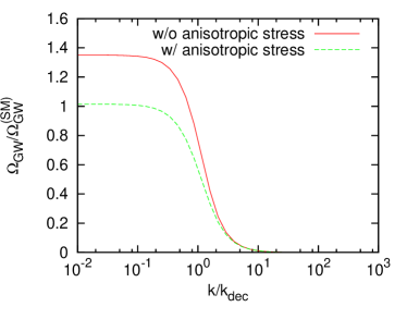
Figure 3: $\Omega_{\rm GW}(k)/\Omega_{\rm GW}^{\rm(SM)}(k)$ as a function of $k$ (normalized by $k_{\rm dec}$) for $B_{X}=0.26$. The green (dotted) line is the full result, taking account of the effect of anisotropic stress. For comparison, in the solid line (red), we also plot $\Omega_{\rm GW}(k)/\Omega_{\rm GW}^{\rm(SM)}(k)$ without the effect of anisotropic stress. The value at the plateau for $k\ll k_{\rm dec}$ is given by $C_{1}\times C_{2}$ and $C_{1}$ with and without anisotropic stress, respectively.

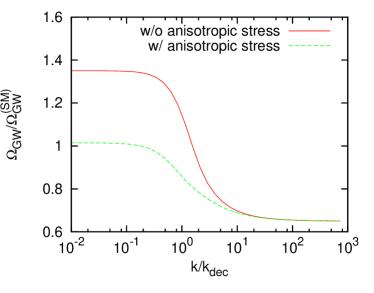
Figure 4: Same as Fig. 3 but for $B_{X}=0.5$.

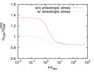
Figure 5: Same as Fig. 3 but for $B_{X}=0.7$.

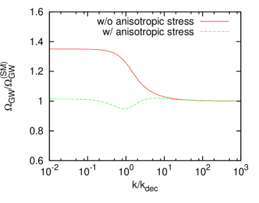
Figure 6: Same as Fig. 3 but for $B_{X}=1.0$.

There are several effects on the GW spectrum in the presence of dark radiation. First, since $\phi$ (nearly) dominates the Universe at the time of its decay in order to realize $\Delta N_{\rm eff}\sim 1$, $\Omega_{\rm GW}$ decreases at $k\gtrsim k_{\rm dec}$. This is due to the change of equation of state of the Universe. The GW energy density scales as $a^{-4}$ inside the horizon, while total energy density scales as $a^{-3}$ in the $\phi$-dominated period. Even if $\phi$ does not completely dominate the Universe, there should be deviation from the radiation-dominated Universe as shown in Fig. 1. Hence high frequency modes entering the horizon before $\phi$-domination experience relative suppression compared with low frequency modes. As a result, as one can see, $\Omega_{\rm GW}$ is suppressed for high frequency modes which enter the horizon before the $\phi$-domination.

In addition, most importantly, the effect of anisotropic stress caused by dark radiation dissipates the GW energy density of the mode with $k\lesssim k_{\rm dec}$, because dark radiation is already created by the $\phi$ decay when such modes enter the horizon. The effect is weaker for higher frequency because the abundance of $X$ is smaller at the horizon entry of high frequency modes.

Therefore, we expect suppression on the GW spectrum for both high frequency and low frequency sides : the former caused by modified expansion rate due to $\phi$ and the latter by the anisotropic stress of $X$. The GW spectrum between these two regimes, $k\sim k_{\rm dec}$, receives both effects and the resulting shape of the spectrum depends on how effective those effects are at $k\sim k_{\rm dec}$. Numerical calculations show that a dip in the spectrum may appear at $k\sim k_{\rm dec}$. In particular, the dip becomes more apparent when $B_{X}$ is close to $1$. Such a dip provides a smoking-gun signature of the dark-radiation production by the decay of massive particles. If $\phi$ and $X$ are completely sequestered from the standard-model sector, for example, $B_{X}=1$ may be realized. Then, such a model provides a striking signature in the GW spectrum.

Note that, in the low frequency limit $k\ll k_{\rm dec}$, we have numerically confirmed the suppression factor $C_{2}$ caused by dark radiation. As a result, $\Omega_{\rm GW}/\Omega_{\rm GW}^{\rm(SM)}$ at $k\ll k_{\rm dec}$ is close to one as shown in Fig. 2.

IV Conclusions and Discussion

In this paper we have studied the spectrum of inflationary GW background in the presence of dark radiation, motivated by recent observational preferences for $\Delta N_{\rm eff}\sim 1$. We have assumed that the dark radiation is non-thermally produced by decay of massive particles $\phi$. There are several effects on the GW spectrum. First, the equation of state of the Universe is modified due to the $\phi$ energy density and it changes the shape of the GW spectrum. Second, the anisotropic stress carried by dark radiation dissipates the GW amplitude for modes entering the horizon around and after $\phi$ decay. Numerical results show that there may appear a characteristic dip around $k\sim k_{\rm dec}$, which is a smoking-gun signature of dark radiation. It not only provides an evidence of dark radiation, but also sheds light on its production mechanism.

Some notes are in order. We have assumed that the dark radiation anisotropic stress is induced only by the primordial GWs. This is not in general true in the second order perturbation theory. Free-streaming particles (as well as other fluids) contribute to GWs at the second order in the scalar perturbation even if there is no primordial tensor perturbation. However, this contribution is negligible for $r\gtrsim 10^{-6}$ Baumann:2007zm ; Mangilli:2008bw .

So far, we have considered dark radiation produced by the decay of $\phi$. However, it is possible that the dark radiation was once in thermal equilibrium and decoupled from thermal bath at the temperature $T_{\rm dec}$. In this case, the extra effective number of neutrino species is given by

$$\Delta N_{\rm eff}=\frac{4}{7}\epsilon N_{X}\left[\frac{10.75}{g_{*s}(T_{\rm dec})}\right]^{4/3},$$ (30)

where

$$\epsilon=\begin{cases}1&{\rm~{}~{}for~{}a~{}real~{}scalar},\\ 7/4&{\rm~{}~{}for~{}a~{}chiral~{}fermion},\end{cases}$$ (31)

and $N_{X}$ counts the number of $X$ species. If the decoupling temperature is higher than the weak scale, we need $N_{X}\gtrsim 20$ for explaining $\Delta N_{\rm eff}\simeq 1$. The modulation in the GW spectrum, similar to the effect caused by of neutrinos apparent at the GW frequency of $10^{-10}$ Hz Weinberg:2003ur ; Watanabe:2006qe , appears at the frequency inside the range of DECIGO/BBO sensitivities for $T_{\rm dec}\sim 10^{7}$–$10^{9}$ GeV. If the decoupling temperature is $\mathcal{O}$(1) MeV, $N_{X}\sim 1$ is sufficient in order to obtain $\Delta N_{\rm eff}\simeq 1$ but the dip in the GW spectrum cannot be seen in the GW detectors. Instead, overall normalization of the GW spectrum at the observable frequency range, inferred from the measured tensor-to-scalar ratio, is enhanced by the factor $C_{1}\sim 1.3$. (At this epoch, dark radiation took part in thermal bath and there is no anisotropic stress damping on GW amplitudes with corresponding modes.) This provides another indirect evidence of dark radiation.

Appendix A Equation of motion of gravitational waves with dark radiation

In this Appendix we derive Eq. (17), the equation of motion of GWs with dark radiation. We follow Refs. Weinberg:2003ur ; Watanabe:2006qe but the result is slightly different because $X$ is continuously produced by the decay of $\phi$ so that the number of $X$ in the comoving volume is not constant.

Throughout this appendix, we use the synchronous gauge and consider tensor perturbations defined in Eq. (11).

The equation of motion for tensor perturbations in Fourier space is

$$\frac{\partial^{2}h_{ij}}{\partial u^{2}}+2H_{u}\frac{\partial h_{ij}}{\partial u}+h_{ij}=16\pi G\left(\frac{a}{k}\right)^{2}\Pi_{ij},$$ (32)

where $u\equiv k\eta\equiv k\int_{0}^{t}\frac{dt^{\prime}}{a(t^{\prime})}$, $H_{u}\equiv\frac{1}{a}\frac{\partial a}{\partial u}$ and $\Pi_{ij}$ is defined by using the total energy momentum tensor as

$$T_{ij}^{\rm(tot)} = Pg_{ij}+a^{2}\Pi_{ij},$$ (33)

$$P \equiv \frac{1}{3}T^{i{\rm(tot)}}_{\;\;i}.$$ (34)

Our goal in this appendix is to express the RHS of Eq. (32) in terms of metric perturbations. In what follows, use the fact that only the collisionless particle (i.e., $X$) contributes to the anisotropic stress $\Pi_{ij}$.

We first introduce the distribution function of the relativistic components $F^{\rm(tot)}(t,x^{i},p_{i})$, with which the total number of relativistic particles with particular momentum range contained in the volume element is given by $F^{\rm(tot)}dx^{1}dx^{2}dx^{3}dp_{1}dp_{2}dp_{3}$. (Here and hereafter, $x^{i}$ is the comoving coordinate, while $p_{i}$ is the comoving momentum.) Note that $F^{\rm(tot)}$ is a scalar under general coordinate transformations which preserve the synchronous gauge. The distribution function can be decomposed as

$$F^{\rm(tot)}(t,x^{i},p_{i})=F^{(X)}(t,x^{i},p_{i})+F^{\rm(rad)}(t,x^{i},p_{i}),$$ (35)

where $F^{(X)}$ and $F^{\rm(rad)}$ are distribution functions of the dark radiation $X$ and that of ordinary radiation (like photon, gluon, and so on) with very short free-streaming length, respectively. Hereafter, we omit the superscript $X$ for the distribution function of $X$ for notational simplicity : $F(t,x^{i},p_{i})\equiv F^{(X)}(t,x^{i},p_{i})$.

We start with the effect of dark radiation on the anisotropic stress. The distribution function of $X$ obeys the collisionless Boltzmann equation with source from non-relativistic decaying particle $\phi$:

$$\frac{dF}{dt}=\frac{B_{X}}{4\pi(p^{0})^{3}}\Gamma_{\phi}\rho_{\phi}\delta\left(p^{0}-\frac{m_{\phi}}{2}\right),$$ (36)

where $p^{0}$ is the energy of $X$, and we assume that $\phi$ decays into two $X$s. Also note that $p^{0}$ and $p^{i}$ should be regarded as functions of $p_{i}$ through $g_{\mu\nu}p^{\mu}p^{\nu}=-(p^{0})^{2}+a^{2}(\delta_{ij}+h_{ij})p^{i}p^{j}=0$ and $p^{i}=g^{ij}p_{j}=a^{-2}(\delta_{ij}-h_{ij})p_{j}$. The LHS of Eq. (36) is

$$\begin{split}\frac{dF}{dt}&=\frac{\partial F}{\partial t}+\frac{dx^{i}}{dt}\frac{\partial F}{\partial x^{i}}+\frac{dp_{i}}{dt}\frac{\partial F}{\partial p_{i}}\\ &=\frac{\partial F}{\partial t}+\frac{p^{i}}{p^{0}}\frac{\partial F}{\partial x^{i}}+\frac{1}{2}g_{ij,k}\frac{p^{i}p^{j}}{p^{0}}\frac{\partial F}{\partial p_{k}},\end{split}$$ (37)

where we used

$$\frac{dx^{i}}{dt} = \frac{p^{i}}{p^{0}},$$ (38)

$$\frac{dp_{i}}{dt} = \frac{1}{2}g_{jk,i}\frac{p^{j}p^{k}}{p^{0}}.$$ (39)

Eq. (39) is obtained from the geodesic equation.

Next we decompose $F$ into the unperturbed part $\bar{F}(t,p)$, where $p\equiv\sqrt{p_{i}p_{i}}$ should not be confused with the pressure, and the perturbed part $\delta F$. We further decompose $\delta F$ into two terms $\delta F_{1}$ and $\delta F_{2}$ for later convenience:

$$\delta F_{1}(t,x^{i},p_{i}) \equiv \bar{F}(t,(g^{ij}p_{i}p_{j})^{1/2}/a)-\bar{F}(t,p),$$

$$\delta F_{2}(t,x^{i},p_{i}) \equiv F-\bar{F}-\delta F_{1}.$$ (41)

We get from Eq. (36) the zeroth-order equation

$$\frac{\partial\bar{F}}{\partial t}=\frac{B_{X}}{4\pi(\bar{p}^{0})^{3}}\Gamma_{\phi}\rho_{\phi}\delta\left(\bar{p}^{0}-\frac{m_{\phi}}{2}\right),$$ (42)

and the first-order one

$$\frac{\partial(\delta F_{1}+\delta F_{2})}{\partial t}+\frac{\bar{p}^{i}}{\bar{p}^{0}}\frac{\partial(\delta F_{1}+\delta F_{2})}{\partial x^{i}}$$

$$+\frac{1}{2}(\delta g_{jk})_{,i}\frac{\bar{p}^{j}\bar{p}^{k}}{\bar{p}^{0}}\frac{\partial\bar{F}}{\partial p_{i}}=a\frac{\partial^{2}\bar{F}}{\partial p\partial t}\delta p^{0}.$$ (43)

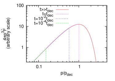
Figure 7: $4\pi p^{3}\bar{F}$ as functions of $p$ (normalized by $p_{\rm dec}\equiv a(t_{\rm dec})m_{\phi}/2$). Each line corresponds to $t\gg t_{\rm dec}$ (red solid), $t=10^{-4}t_{\rm dec}$ (green long-dashed), $10^{-2}t_{\rm dec}$ (blue short-dotted) and $t_{\rm dec}$(magenta dotted).

In Fig. 7, we show $4\pi p^{3}\bar{F}$ as a function of $p/p_{\rm dec}$, where $p_{\rm dec}\equiv a(t_{\rm dec})m_{\phi}/2$ is the comoving momentum of $X$ produced at $t=t_{\rm dec}$. We can see that the energy fraction $4\pi p^{3}\bar{F}$ is mostly carried by $X$ produced at $t\simeq t_{\rm dec}$. Then we use the following equations:

$$\delta F_{1} = -\frac{1}{2}h_{ij}\frac{p_{i}p_{j}}{p}\frac{\partial\bar{F}}{\partial p},$$ (44)

$$\delta p^{0} = -\frac{1}{2a}\frac{h_{ij}p_{i}p_{j}}{p},$$ (45)

$$\delta p^{i} = -\frac{1}{a^{2}}h_{ij}p_{j}.$$ (46)

Using $\hat{p}_{i}\equiv p_{i}/p$ and substituting Eq. (44) – Eq. (46) into Eq. (43), we get

$$\frac{\partial\delta F_{2}}{\partial t}+\frac{\hat{p}_{i}}{a}\frac{\partial\delta F_{2}}{\partial x^{i}}=\frac{1}{2}\frac{\partial h_{ij}}{\partial t}\frac{\partial\bar{F}}{\partial p}p\hat{p}_{i}\hat{p}_{j}.$$ (47)

In terms of conformal time $\eta$, this equation is expressed as

$$\frac{\partial\delta F_{2}}{\partial\eta}+\hat{p}_{i}\frac{\partial\delta F_{2}}{\partial x^{i}}=\frac{1}{2}\frac{\partial h_{ij}}{\partial\eta}\frac{\partial\bar{F}}{\partial p}p\hat{p}_{i}\hat{p}_{j}.$$ (48)

In Fourier space,

$$\frac{\partial\delta F_{2}}{\partial\eta}+ik\mu\delta F_{2}=\frac{1}{2}\frac{\partial h_{ij}}{\partial\eta}\frac{\partial\bar{F}}{\partial p}p\hat{p}_{i}\hat{p}_{j},$$ (49)

where

$$\delta F_{2}(\eta,x^{i},p_{i}) = \int\frac{d^{3}k}{(2\pi)^{3}}\delta F_{2}(\eta,k_{i},p_{i})e^{ik_{i}x^{i}},$$ (50)

$$h_{ij}(\eta,x^{i}) = \int\frac{d^{3}k}{(2\pi)^{3}}h_{ij}(\eta,k_{i})e^{ik_{i}x^{i}},$$ (51)

$$\mu \equiv \hat{k}_{i}\hat{p}_{i}.$$ (52)

We can use line-of-sight integral to get the solution of Eq. (49):

$$\delta F_{2}=\int_{0}^{\eta}d\eta^{\prime}\frac{1}{2}\frac{\partial h_{ij}}{\partial\eta}(\eta^{\prime})\frac{\partial\bar{F}}{\partial p}(\eta^{\prime})p\hat{p}_{i}\hat{p}_{j}e^{-ik\mu(\eta-\eta^{\prime})},$$ (53)

where we have used $\delta F_{2}(\eta=0)=0$ because there is no $X$ in the beginning.

We take the first-order perturbation of the energy-momentum tensor of $X$:

$$T_{\mu\nu}^{(X)} = \frac{1}{\sqrt{-{\rm det}g_{\mu\nu}}}\int d^{3}pF\frac{p_{\mu}p_{\nu}}{p^{0}},$$ (54)

$$\delta T_{ij}^{(X)} = \frac{1}{a^{3}}\int d^{3}p\left[(\delta F_{1}+\delta F_{2})\frac{p_{i}p_{j}}{\bar{p}^{0}}+\bar{F}p_{i}p_{j}\delta\left(\frac{1}{p^{0}}\right)\right].$$

Note that energy momentum tensor defined above transforms as a tensor under general coordinate transformations since $\int d^{3}p/p^{0}\propto d^{4}p\delta(g^{\mu\nu}p_{\mu}p_{\nu})$. Using Eq. (44) – Eq. (46), we get

$$\delta T_{ij}^{(X)} = \frac{1}{a^{3}}\int d^{3}p\left[\frac{}{}\delta F_{2}ap\hat{p}_{i}\hat{p}_{j}\right.$$ (56)

$$\left.-\frac{1}{2}ah_{kl}p^{2}\hat{p}_{i}\hat{p}_{j}\hat{p}_{k}\hat{p}_{l}\frac{\partial\bar{F}}{\partial p}+\frac{1}{2}ah_{kl}p\hat{p}_{i}\hat{p}_{j}\hat{p}_{k}\hat{p}_{l}\bar{F}\right]$$

$$= \frac{1}{a^{3}}\int d^{3}p\delta F_{2}ap\hat{p}_{i}\hat{p}_{j}$$

$$+\frac{1}{a^{3}}\int dpp^{2}\left[-\frac{1}{2}ah_{kl}p^{2}\frac{\partial\bar{F}}{\partial p}+\frac{1}{2}ah_{kl}p\bar{F}\right]$$

$$\times\frac{4\pi}{15}(\delta_{ij}\delta_{kl}+\delta_{ik}\delta_{jl}+\delta_{il}\delta_{jk})$$

$$= \frac{1}{a^{2}}\int d^{3}p\delta F_{2}p\hat{p}_{i}\hat{p}_{j}+\frac{1}{3}a^{2}h_{ij}\rho_{X}.$$

Here, we used

$$\int d\Omega_{p}\hat{p}_{i}\hat{p}_{j}\hat{p}_{k}\hat{p}_{l}e^{-i\hat{p}_{i}\hat{k}_{i}u}$$

$$=4\pi\left[j_{4}(u)\hat{k}_{i}\hat{k}_{j}\hat{k}_{k}\hat{k}_{l}-\frac{j_{3}(u)}{u}(\hat{k}_{i}\hat{k}_{j}\delta_{kl}+{\rm 5~{}perms})\right.$$

$$\;\;\;+\left.\frac{j_{2}(u)}{u^{2}}(\delta_{ij}\delta_{kl}+{\rm 2~{}perms})\right]$$ (57)

and

$$\int dp4\pi p^{3}\bar{F}=a^{4}\rho_{X},$$ (58)

where $\rho_{X}$ is the energy density of $X$ and $j_{n}$ is the $n$-th spherical Bessel function.

Next, we consider the effect of $F^{\rm(rad)}$, for which $\delta F_{2}^{\rm(rad)}=0$ because the free-streaming length is very short. Then, we obtain

$$\delta T_{ij}^{\rm(rad)}=\frac{1}{3}a^{2}h_{ij}\rho_{\rm rad}.$$ (59)

We also note that perturbation in the energy momentum tensor of $\phi$ vanishes since it behaves as non-relativistic matter :

$$\delta T_{ij}^{\rm(\phi)}=0.$$ (60)

Taking the first-order perturbation of Eq. (34), we obtain

$$\delta T_{ij}^{\rm(tot)} = \delta P\cdot\bar{g}_{ij}+\bar{P}\cdot\delta g_{ij}+a^{2}\Pi_{ij}$$ (61)

$$= \frac{1}{3}a^{2}h_{ij}(\rho_{X}+\rho_{\rm rad})+a^{2}\Pi_{ij},$$

where we used Eq. (44) – Eq. (46), Eq. (53), Eq. (57), $h_{ii}=0$ and $\delta P=0$. The last condition comes from the fact that tensor perturbations cannot produce perturbations in scalar variables. Using Eq. (56), Eq. (59), Eq. (60), and Eq. (61), we obtain

$$a^{2}\Pi_{ij}=\frac{1}{a^{2}}\int d^{3}p\delta F_{2}p\hat{p}_{i}\hat{p}_{j}.$$ (62)

Substituting Eq. (62) into the RHS of Eq. (32), we obtain

$$\frac{\partial^{2}h_{ij}}{\partial u^{2}}+2H_{u}\frac{\partial h_{ij}}{\partial u}+h_{ij}$$

$$=16\pi G\left(\frac{a}{k}\right)^{2}\frac{1}{a^{4}}\int d^{3}pp\hat{p}_{i}\hat{p}_{j}$$

$$\;\;\;\times\int_{0}^{\eta}d\eta^{\prime}\frac{1}{2}\frac{\partial h_{kl}}{\partial\eta}(\eta^{\prime})\frac{\partial\bar{F}}{\partial p}(\eta^{\prime})p\hat{p}_{k}\hat{p}_{l}e^{-ik\mu(\eta-\eta^{\prime})}$$

$$=-8\pi G\frac{1}{k^{2}a^{2}}\int_{0}^{\eta}d\eta^{\prime}\frac{\partial h_{kl}}{\partial\eta}(\eta^{\prime})$$

$$\;\;\;\int d\Omega_{p}\frac{1}{\pi}a^{4}\rho_{X}(\eta^{\prime})\hat{p}_{i}\hat{p}_{j}\hat{p}_{k}\hat{p}_{l}e^{-ik\mu(\eta-\eta^{\prime})}$$

$$=-24H_{u}^{2}\frac{1}{a^{4}\rho_{\rm tot}(u)}\int_{0}^{u}du^{\prime}a^{4}\rho_{X}(u^{\prime})\frac{\partial h_{ij}}{\partial u}(u^{\prime})\frac{j_{2}(u-u^{\prime})}{(u-u^{\prime})^{2}},$$

where we used partial integration, Eq. (57) and Friedmann equation $H_{u}^{2}=8\pi G\rho_{\rm tot}a^{2}/3k^{2}$. After decomposing $h_{ij}$ using Eq. (12), we finally obtain Eq. (17).

References

- (1) G. Mangano, G. Miele, S. Pastor, T. Pinto, O. Pisanti and P. D. Serpico, Nucl. Phys. B 729, 221 (2005) [hep-ph/0506164].
- (2) Y. I. Izotov and T. X. Thuan, Astrophys. J. 710, L67 (2010) [arXiv:1001.4440 [astro-ph.CO]].
- (3) E. Aver, K. A. Olive and E. D. Skillman, JCAP 1005, 003 (2010) [arXiv:1001.5218 [astro-ph.CO]]; JCAP 1204, 004 (2012) [arXiv:1112.3713 [astro-ph.CO]].
- (4) E. Komatsu et al. [ WMAP Collaboration ], Astrophys. J. Suppl. 192, 18 (2011). [arXiv:1001.4538 [astro-ph.CO]].
- (5) J. Dunkley et al., Astrophys. J. 739, 52 (2011) [arXiv:1009.0866 [astro-ph.CO]].
- (6) R. Keisler et al., Astrophys. J. 743, 28 (2011) [arXiv:1105.3182 [astro-ph.CO]].
- (7) M. Archidiacono, E. Calabrese and A. Melchiorri, Phys. Rev. D 84, 123008 (2011) [arXiv:1109.2767 [astro-ph.CO]].
- (8) E. Calabrese, M. Archidiacono, A. Melchiorri and B. Ratra, arXiv:1205.6753 [astro-ph.CO].
- (9) J. Hamann, JCAP 1203, 021 (2012) [arXiv:1110.4271 [astro-ph.CO]].
- (10) K. M. Nollett and G. P. Holder, arXiv:1112.2683 [astro-ph.CO].
- (11) J. Hamann, S. Hannestad, G. G. Raffelt, I. Tamborra and Y. Y. Y. Wong, Phys. Rev. Lett. 105, 181301 (2010) [arXiv:1006.5276 [hep-ph]].
- (12) J. Hamann, S. Hannestad, G. G. Raffelt and Y. Y. Y. Wong, JCAP 1109, 034 (2011) [arXiv:1108.4136 [astro-ph.CO]].
- (13) K. Ichikawa, M. Kawasaki, K. Nakayama, M. Senami and F. Takahashi, JCAP 0705, 008 (2007) [hep-ph/0703034 [HEP-PH]].
- (14) J. Jaeckel, J. Redondo and A. Ringwald, Phys. Rev. Lett. 101, 131801 (2008) [arXiv:0804.4157 [astro-ph]].
- (15) K. Nakayama, F. Takahashi and T. T. Yanagida, Phys. Lett. B 697, 275 (2011) [arXiv:1010.5693 [hep-ph]].
- (16) W. Fischler and J. Meyers, Phys. Rev. D 83, 063520 (2011) [arXiv:1011.3501 [astro-ph.CO]].
- (17) M. Kawasaki, N. Kitajima and K. Nakayama, Phys. Rev. D 83, 123521 (2011) [arXiv:1104.1262 [hep-ph]].
- (18) J. P. Hall and S. F. King, JHEP 1106, 006 (2011) [arXiv:1104.2259 [hep-ph]].
- (19) J. Hasenkamp, Phys. Lett. B 707, 121 (2012) [arXiv:1107.4319 [hep-ph]].
- (20) M. Kawasaki, K. Miyamoto, K. Nakayama and T. Sekiguchi, JCAP 1202, 022 (2012) [arXiv:1107.4962 [astro-ph.CO]].
- (21) J. L. Menestrina and R. J. Scherrer, Phys. Rev. D 85, 047301 (2012) [arXiv:1111.0605 [astro-ph.CO]].
- (22) T. Kobayashi, F. Takahashi, T. Takahashi and M. Yamaguchi, JCAP 1203, 036 (2012) [arXiv:1111.1336 [astro-ph.CO]].
- (23) D. Hooper, F. S. Queiroz and N. Y. Gnedin, Phys. Rev. D 85, 063513 (2012) [arXiv:1111.6599 [astro-ph.CO]].
- (24) K. S. Jeong and F. Takahashi, arXiv:1201.4816 [hep-ph].
- (25) E. Kawakami, M. Kawasaki, K. Miyamoto, K. Nakayama and T. Sekiguchi, JCAP 1207, 037 (2012) [arXiv:1202.4890 [astro-ph.CO]].
- (26) M. Blennow, E. Fernandez-Martinez, O. Mena, J. Redondo and P. Serra, arXiv:1203.5803 [hep-ph].
- (27) T. Moroi and M. Takimoto, arXiv:1207.4858 [hep-ph].
- (28) W. Zhao, Y. Zhang and T. Xia, Phys. Lett. B 677, 235 (2009) [arXiv:0905.3223 [astro-ph.CO]].
- (29) S. Weinberg, Phys. Rev. D 69, 023503 (2004) [astro-ph/0306304].
- (30) D. A. Dicus and W. W. Repko, Phys. Rev. D 72, 088302 (2005) [astro-ph/0509096].
- (31) Y. Watanabe and E. Komatsu, Phys. Rev. D 73, 123515 (2006) [astro-ph/0604176].
- (32) K. Ichiki, M. Yamaguchi and J. ’I. Yokoyama, Phys. Rev. D 75, 084017 (2007) [hep-ph/0611121].
- (33) N. Seto, S. Kawamura and T. Nakamura, Phys. Rev. Lett. 87, 221103 (2001) [astro-ph/0108011]; S. Kawamura et al., Class. Quant. Grav. 28, 094011 (2011).
- (34) J. Crowder and N. J. Cornish, Phys. Rev. D 72, 083005 (2005) [gr-qc/0506015].
- (35) C. Cutler and D. E. Holz, Phys. Rev. D 80, 104009 (2009) [arXiv:0906.3752 [astro-ph.CO]].
- (36) M. S. Turner and F. Wilczek, Phys. Rev. Lett. 65, 3080 (1990).
- (37) N. Seto and J. ’I. Yokoyama, J. Phys. Soc. Jap. 72, 3082 (2003) [gr-qc/0305096].
- (38) H. Tashiro, T. Chiba and M. Sasaki, Class. Quant. Grav. 21, 1761 (2004) [gr-qc/0307068].
- (39) L. A. Boyle and P. J. Steinhardt, Phys. Rev. D 77, 063504 (2008) [astro-ph/0512014].
- (40) L. A. Boyle and A. Buonanno, Phys. Rev. D 78, 043531 (2008) [arXiv:0708.2279 [astro-ph]].
- (41) K. Nakayama, S. Saito, Y. Suwa and J. ’i. Yokoyama, Phys. Rev. D 77, 124001 (2008) [arXiv:0802.2452 [hep-ph]].
- (42) K. Nakayama, S. Saito, Y. Suwa and J. ’i. Yokoyama, JCAP 0806, 020 (2008) [arXiv:0804.1827 [astro-ph]].
- (43) S. Kuroyanagi, T. Chiba and N. Sugiyama, Phys. Rev. D 79, 103501 (2009) [arXiv:0804.3249 [astro-ph]].
- (44) S. Mukohyama, K. Nakayama, F. Takahashi and S. Yokoyama, Phys. Lett. B 679, 6 (2009) [arXiv:0905.0055 [hep-th]].
- (45) K. Nakayama and J. ’i. Yokoyama, JCAP 1001, 010 (2010) [arXiv:0910.0715 [astro-ph.CO]].
- (46) K. Nakayama and F. Takahashi, JCAP 1011, 009 (2010) [arXiv:1008.2956 [hep-ph]].
- (47) S. Schettler, T. Boeckel and J. Schaffner-Bielich, Phys. Rev. D 83, 064030 (2011) [arXiv:1010.4857 [astro-ph.CO]].
- (48) R. Durrer and J. Hasenkamp, Phys. Rev. D 84, 064027 (2011) [arXiv:1105.5283 [gr-qc]].
- (49) S. Kuroyanagi, K. Nakayama and S. Saito, Phys. Rev. D 84, 123513 (2011) [arXiv:1110.4169 [astro-ph.CO]].
- (50) R. Jinno, T. Moroi and K. Nakayama, Phys. Lett. B 713, 129 (2012) [arXiv:1112.0084 [hep-ph]].
- (51) R. Saito and S. Shirai, Phys. Lett. B 713, 237 (2012) [arXiv:1201.6589 [hep-ph]].
- (52) K. Rajagopal, M. S. Turner and F. Wilczek, Nucl. Phys. B 358, 447 (1991).
- (53) R. D. Peccei and H. R. Quinn, Phys. Rev. Lett. 38, 1440 (1977).
- (54) For reviews, see J. E. Kim, Phys. Rept. 150, 1 (1987); J. E. Kim and G. Carosi, Rev. Mod. Phys. 82, 557 (2010) [arXiv:0807.3125 [hep-ph]].
- (55) E. J. Chun and A. Lukas, Phys. Lett. B 357, 43 (1995) [hep-ph/9503233].
- (56) G. F. Giudice and A. Strumia, Nucl. Phys. B 858, 63 (2012) [arXiv:1108.6077 [hep-ph]].
- (57) G. Aad et al. [The ATLAS Collaboration], arXiv:1207.7214 [hep-ex]; S. Chatrchyan et al. [The CMS Collaboration], arXiv:1207.7235 [hep-ex].
- (58) P. Graf and F. D. Steffen, Phys. Rev. D 83, 075011 (2011) [arXiv:1008.4528 [hep-ph]].
- (59) For a review, see M. Maggiore, Phys. Rept. 331, 283 (2000) [gr-qc/9909001].
- (60) B. Allen, Phys. Rev. D 37, 2078 (1988).
- (61) V. Sahni, Phys. Rev. D 42, 453 (1990).
- (62) M. S. Turner, M. J. White and J. E. Lidsey, Phys. Rev. D 48, 4613 (1993) [astro-ph/9306029].
- (63) M. S. Turner, Phys. Rev. D 55, 435 (1997) [astro-ph/9607066].
- (64) T. L. Smith, M. Kamionkowski and A. Cooray, Phys. Rev. D 73, 023504 (2006) [astro-ph/0506422].
- (65) T. L. Smith, H. V. Peiris and A. Cooray, Phys. Rev. D 73, 123503 (2006) [astro-ph/0602137].
- (66) S. Chongchitnan and G. Efstathiou, Phys. Rev. D 73, 083511 (2006) [astro-ph/0602594].
- (67) B. C. Friedman, A. Cooray and A. Melchiorri, Phys. Rev. D 74, 123509 (2006) [astro-ph/0610220].
- (68) T. L. Smith, M. Kamionkowski and A. Cooray, Phys. Rev. D 78, 083525 (2008) [arXiv:0802.1530 [astro-ph]].
- (69) D. Baumann, P. J. Steinhardt, K. Takahashi and K. Ichiki, Phys. Rev. D 76, 084019 (2007) [hep-th/0703290].
- (70) A. Mangilli, N. Bartolo, S. Matarrese and A. Riotto, Phys. Rev. D 78, 083517 (2008) [arXiv:0805.3234 [astro-ph]].