Charged di-boson production at the LHC
in a 4–site model with a composite Higgs boson

Abstract

We investigate the scope of the LHC in probing the parameter space of a 4-site model supplemented by one composite Higgs state, assuming all past, current and future energy and luminosity stages of the CERN machine. We concentrate on the yield of charged di-boson production giving two opposite-charge different-flavour leptons and missing (transverse) energy, i.e., events induced via the subprocess $q\bar{q}\rightarrow e^{+}\nu_{e}\mu^{-}\bar{\nu}_{\mu}$ + ${\rm{c.c.}}$, which enables the production in the intermediate step of all additional neutral and charged gauge bosons belonging to the spectrum of this model, some of which in resonant topologies. We find this channel accessible over the background at all LHC configurations after a dedicated cut-based analysis. We finally compare the yield of the di-boson mode to that of Drell-Yan processes and establish that they have complementary strengths, one covering regions of parameter space precluded to the others and vice versa.

I Introduction

A strong Electro-Weak (EW) sector is expected to produce a variety of bound states including particles of spin zero and spin one, like the $\sigma$, the $\rho$ and the $a_{1}$ emerging from quark states within Quantum Chromo-Dynamics (QCD). Just like in QCD, the phenomenology below the scale of the strong EW interactions producing similar resonances can be studied in terms of an effective Lagrangian containing these additional degrees of freedom, based on the observed symmetries of the EW sector. Effective terms adding to the chiral Lagrangian just a simple scalar state or a scalar and a vector state have been recently suggested Contino et al. (2010); Espinosa et al. (2012a); Bellazzini et al. (2012); Gillioz et al. (2012). These formulations are useful because they allow for a general parameterisation of the (strongly) broken symmetry of the EW sector. These new resonances also appear in five-dimensional extensions of the Standard Model (SM) as Kaluza-Klein (KK) excitations of the SM gauge bosons Agashe et al. (2003); Csaki et al. (2004a, b); Barbieri et al. (2004); Cacciapaglia et al. (2004a, b). When deconstructed Arkani-Hamed et al. (2001a, b); Hill et al. (2001); Cheng et al. (2001); Abe et al. (2003); Falkowski and Kim (2002); Randall et al. (2003); Son and Stephanov (2004); de Blas et al. (2006) these theories emerge as gauge theories with extended $SU(2)$ symmetries. Simple four-dimensional models, like the 3-site Chivukula et al. (2006), the 4-site Accomando et al. (2009) and the effective composite Higgs model Contino et al. (2007) can be used to characterise the main features of the emerging phenomenology.

In its original formulation, the 4-site model describes in an effective way the interactions of extra spin-one resonances as gauge fields of a $SU(2)\otimes SU(2)$ extra gauge group. They can be thought of as the first KK excitations emerging from a five-dimensional formulation, and, due to the Anti-de Sitter/Conformal Field Theory (AdS/CFT) correspondence, they are composite states of a strong dynamics also responsible for the breaking of the EW symmetry. As stated before, a strong EW sector is expected to produce also new scalar and fermion particles as bound states. In this note we consider the inclusion of a new scalar field, singlet under the gauge group, in order to reproduce in our effective description, the scalar particle recently detected by the ATLAS and CMS experiments at the Large Hadron Collider (LHC) Incandela (July 4, 2012); Gianotti (July 4, 2012). The couplings of our composite Higgs particle to the SM and extra gauge bosons are free parameters for which we will derive bounds due to the EW precision tests and the present LHC measurements, as well as theoretical constraints enforced by perturbative unitarity requirement.

It is the purpose of this paper to investigate, in the context of the 4-site model with one composite Higgs state, the phenomenology of charged di-boson production at the LHC, yielding opposite-charge different-flavour lepton pairs and missing transverse energy, i.e., the process

$$pp(q\bar{q})\rightarrow W^{+}W^{-}\rightarrow e^{+}\nu_{e}\mu^{-}\bar{\nu}_{\mu}~{}+~{}{\rm{c.c.}}\rightarrow e^{\pm}\mu^{\mp}E_{T}^{\rm miss}$$ (1)

wherein the symbol $W^{\pm}$ refers to any possible charged spin 1 massive gauge bosons present in the model, which also allows for the production of intermediate neutral spin 1 massless (i.e., the photon) and massive gauge bosons. In fact, having inserted a light composite Higgs state in the 4-site model, one also ought to investigate the yield of the process

$$pp(gg)\rightarrow h\rightarrow W^{+}W^{-}\rightarrow e^{+}\nu_{e}\mu^{-}\bar{\nu}_{\mu}~{}+~{}{\rm{c.c.}}\rightarrow e^{\pm}\mu^{\mp}E_{T}^{\rm miss}$$ (2)

where, however, having fixed $m_{h}=125$ GeV (to account for the recent LHC results), implies that the charged gauge bosons produced in intermediate stages can only be the SM ones.

In performing our analysis, we will take into account experimental constraints from EW Precision Test (EWPT) data produced at LEP, SLC and Tevatron as well as experimental limits from direct searches of Higgs (as mentioned) and new gauge bosons performed at Tevatron and LHC via Drell-Yan (DY) channels. In the attempt to extract a signal of the model, we will focus our attention to all energy and luminosity stages covered already or still foreseen for the CERN machine. Ultimately, we will want to contrast the discovery potential of the LHC of charged di-boson production events with that of DY events, building on previous studies of some of us.

The plan of the paper is as follows. In the next section we recall the details of the construction of the 4-site model and its relation with the general effective description of vector and axial-vector resonances. In this framework, the inclusion of a singlet composite scalar state is straightforward. We then describe the parameter space of the model and derive both theoretical and experimental bounds constraining it. Sect. III will instead be devoted to describe the production and decay dynamics of processes (1)–(2), eventually extracting from these exclusion and evidence/discovery limits over the surviving parameter space. A final section will be devoted to summarise our work and conclude on the comparison of the relative yields of DY and di-boson processes.

II The 4-site model with a singlet composite scalar state

The 4-site model is a moose model based on the $SU(2)_{L}\otimes SU(2)_{1}\otimes SU(2)_{2}\otimes U(1)_{Y}$ gauge symmetry and contains three non-linear $\sigma$-model fields interacting with the gauge fields, which trigger spontaneous EW Symmetry Breaking (EWSB). Its construction is presented in Accomando et al. (2009) while some of its phenomenological consequences are analysed in Accomando et al. (2011a, b, c); Accomando et al. (2012).

In order to extend the 4-site model to include a new singlet scalar field, let us start by briefly reviewing its relation with the general $SU(2)_{L}\otimes SU(2)_{R}$ invariant Lagrangian describing vector and axial-vector resonances. Vector and axial-vector resonances, interacting with the SM gauge vector bosons, can be introduced as in Casalbuoni et al. (1989), by assuming, in addition to the standard global symmetry $SU(2)_{L}\otimes SU(2)_{R}$, a local symmetry $SU(2)$ for each new vector resonance. This symmetry group $G\otimes H$, with

$$G=[SU(2)_{L}\otimes SU(2)_{R}]_{\rm global},~{}~{}~{}H=[SU(2)_{L}\otimes SU(2)_{R}]_{\rm local},$$ (3)

spontaneously broken down to the custodial $SU(2)$. Further, we can add to this sector a singlet under the symmetry describing a possible composite Higgs state.

The methods to construct such a Lagrangian are the standard ones used to build up non-linear realisations (see Refs. Coleman et al. (1969); Callan et al. (1969); Bando et al. (1988)). The necessary Goldstone bosons are described by three independent $SU(2)$ elements: $L$, $R$ and $M$, whose transformation properties with respect to $G\otimes H$ are the following

$$L^{\prime}(x)=g_{L}L(x)h_{L}(x),~{}~{}~{}R^{\prime}(x)=g_{R}R(x)h_{R}(x),$$

$$M^{\prime}(x)=h_{R}(x)^{\dagger}M(x)h_{L}(x),$$ (4)

where $g_{L,R}\in G$ and $h_{L,R}\in H$. These properties are very reminiscent of the linear moose field transformations Casalbuoni et al. (2004). Beside the invariance under $G\otimes H$, we will also require an invariance under the following discrete left-right symmetry, denoted by $P$, $L\leftrightarrow R,\,M\leftrightarrow M^{\dagger},$ which ensures that the low-energy theory is parity conserving.

The vector and axial-vector resonances are introduced as linear combinations of the gauge particles associated to the local group $H$. The most general $G\otimes H\otimes P$ invariant Lagrangian is given by Casalbuoni et al. (1989)

$${\cal L}_{R}={\cal L}_{G}+{\cal L}_{kin},$$ (5)

where

$${\cal L}_{G}=-\frac{v^{2}}{4}f({\bf L}_{\mu},{\bf R}_{\mu}),$$ (6)

with

$$f({\bf L}_{\mu},{\bf R}_{\mu})=aI_{1}+bI_{2}+cI_{3}+dI_{4},$$ (7)

$$I_{1}=tr[(V_{0}-V_{1}-V_{2})^{2}], I_{2}=tr[(V_{0}+V_{2})^{2}],$$

$$I_{3}=tr[(V_{0}-V_{2})^{2}], I_{4}=tr[V_{1}^{2}],$$ (8)

and

$$V_{0}^{\mu} = L^{\dagger}D^{\mu}L,$$

$$V_{1}^{\mu} = M^{\dagger}D^{\mu}M,$$

$$V_{2}^{\mu} = M^{\dagger}(R^{\dagger}D^{\mu}R)M.$$ (9)

The parameters $a$, $b$, $c$, $d$ are not all independent and are fixed so that, when decoupling the new resonances, one recovers the SM:

$$a+\frac{cd}{c+d}=1.$$ (10)

The covariant derivatives are defined by

$$D_{\mu}L = \partial_{\mu}L-L{\bf L}_{\mu},$$

$$D_{\mu}R = \partial_{\mu}R-R{\bf R}_{\mu},$$

$$D_{\mu}M = \partial_{\mu}M-M{\bf L}_{\mu}+{\bf R}_{\mu}M,$$ (11)

where ${\bf L}_{\mu}=ig"/\sqrt{2}\tau^{a}/2L_{\mu}^{a}$ and ${\bf R}_{\mu}=ig"/\sqrt{2}\tau^{a}/2R_{\mu}^{a}$ are the gauge fields associated to the local symmetry group $H$. The quantities $V_{i}^{\mu}~{}~{}(i=0,1,2)$ are, by construction, invariant under the global symmetry $G$ and covariant under the gauge group $H$,

$$(V_{i}^{\mu})^{\prime}=h_{L}^{\dagger}V_{i}^{\mu}h_{L},$$ (12)

while their transformation properties under the parity operation, $P$, are:

$$(V_{0}\pm V_{2})\rightarrow\pm M(V_{0}\pm V_{2})M^{\dagger},~{}~{}~{}~{}V_{1}\rightarrow-MV_{1}M^{\dagger}.$$ (13)

Out of the $V_{i}^{\mu}$’s one can build six independent quadratic invariants, which reduce to the four $I_{i}$’s listed above, when parity is enforced. The kinetic part for the vector fields (${\cal L}_{kin}$ in eq. (5)) is written in the standard form.

The 4-site model corresponds to the particular choice:

$$a=0,\,\,\,b=c=\frac{2f_{1}^{2}}{v^{2}},\,\,\,d=\frac{4f_{2}^{2}}{v^{2}},\,\,\,g^{\prime\prime}=\frac{g_{1}}{\sqrt{2}}$$ (14)

and to the following identification of the chiral fields:

$$\Sigma_{1}=L,\,\,\Sigma_{2}=M^{\dagger},\,\,\Sigma_{3}=R.$$ (15)

Therefore the Lagrangian for the sector of spin 1 particles of the 4-site model, is given by:

$${\cal L}_{G} = -\frac{v^{2}}{4}\left[\frac{2f_{1}^{2}}{v^{2}}(I_{2}+I_{3})+\frac{4f_{2}^{2}}{v^{2}}I_{4}\right]$$ (16)

$$= f_{1}^{2}[D_{\mu}\Sigma_{1})^{\dagger}D^{\mu}\Sigma_{1}+(D_{\mu}\Sigma_{3})^{\dagger}D^{\mu}\Sigma_{3}]+f_{2}^{2}(D_{\mu}\Sigma_{2})^{\dagger}D^{\mu}\Sigma_{2}$$

$$= \sum_{i=1}^{3}f_{i}^{2}(D_{\mu}\Sigma_{i})^{\dagger}D^{\mu}\Sigma_{i}$$

with

$$D_{\mu}\Sigma_{1}=\partial_{\mu}\Sigma_{1}-i\tilde{g}\tilde{{W}}_{\mu}\Sigma_{1}+i\Sigma_{1}g_{1}\tilde{A}_{\mu}^{1},$$ (17)

$$D_{\mu}\Sigma_{2}=\partial_{\mu}\Sigma_{2}-ig_{1}\tilde{A}_{\mu}^{1}\Sigma_{2}+i\Sigma_{2}g_{1}\tilde{A}_{\mu}^{2},$$

$$D_{\mu}\Sigma_{3}=\partial_{\mu}\Sigma_{3}-ig_{1}\tilde{A}_{\mu}^{2}\Sigma_{3}+i{\tilde{g}^{\prime}}\Sigma_{3}\tilde{{Y}}_{\mu},$$

where $\tilde{A}_{\mu}^{i}=\tilde{A}_{\mu}^{ia}\tau^{a}/2$ and $g_{1}$ are the gauge fields and couplings, $\tilde{{W}}_{\mu}=\tilde{{W}}_{\mu}^{a}\tau^{a}/2$, $\tilde{{Y}}_{\mu}={\tilde{\cal Y}}_{\mu}\tau^{3}/2$ and $\tilde{g}$, ${\tilde{g}^{\prime}}$ are the gauge fields and couplings associated to $SU(2)_{L}$ and $U(1)_{Y}$, respectively. We have also taken into account that the $P$ symmetry implies $f_{1}=f_{3}$. The condition (10) is equivalent to:

$$\frac{4}{v^{2}}=\frac{1}{f^{2}}=\frac{2}{f_{1}^{2}}+\frac{1}{f_{2}^{2}}.$$ (18)

Let us now include a scalar field $h$, singlet under the group $G\otimes H\otimes P$. For the moment we will not be interested in the self-couplings of this field $h$, and we will consider only interaction terms with the vector fields linear or quadratic in $h$. The inclusion of a composite Higgs state was already considered for the general vector and axial-vector model in Casalbuoni et al. (1997). Here we specialize it in the context of the 4-site model.

The inclusion of a singlet $h$, by taking into account only dimension-four operators, is straightforward:

$${\cal L}_{hG} = (2a_{h}\frac{h}{v}+b_{h}\frac{h^{2}}{v^{2}})f_{1}^{2}[D_{\mu}\Sigma_{1})^{\dagger}D^{\mu}\Sigma_{1}+(D_{\mu}\Sigma_{3})^{\dagger}D^{\mu}\Sigma_{3}]$$ (19)

$$+ (2c_{h}\frac{h}{v}+d_{h}\frac{h^{2}}{v^{2}})f_{2}^{2}(D_{\mu}\Sigma_{2})^{\dagger}D^{\mu}\Sigma_{2}.$$

In principle, one could also add dimension-five operators modifying the coupling of the singlet to a pair of gauge bosons and also Yukawa terms $c_{f}m_{f}/v\bar{f}fh$ which could modify the $h$ production and decay properties. More generally one could introduce a singlet field $\rho_{i}$ for each chiral field $\Sigma_{i}$ as in Casalbuoni et al. (1996). We expect the masses of the two heaviest singlets to be related to the scale of the new vector bosons while the scale of the lightest one to the Fermi scale. In our present analysis we however concentrate on the case of only one Higgs state being present in the model spectrum.

II.1 Parameter space

In the unitary gauge, the 4-site model predicts two new triplets of gauge bosons, which acquire mass through the same non-linear symmetry breaking mechanism giving mass to the SM gauge bosons. Let us denote with $W_{i\mu}^{\pm}$ and $Z_{i\mu}$ ($i=1,2$) the four charged and two neutral heavy resonances appearing as a consequence of the gauge group extension, and with $W^{\pm}_{\mu}$, $Z_{\mu}$ and $A_{\mu}$ the SM gauge bosons. Owing to its gauge structure, the 4-site model a priori contains seven free parameters: the $SU(2)_{L}\otimes U(1)_{Y}$ gauge couplings, $\tilde{g}$ and $\tilde{g}^{\prime}$, the extra $SU(2)_{1,2}$ gauge couplings that we assume to be equal, $g_{2}=g_{1}$, due to the $P$ symmetry, the bare masses of lighter ($W_{1}^{\pm},Z_{1}$) and heavier ($W_{2}^{\pm},Z_{2}$) gauge boson triplets, $M_{1,2}$, and their bare direct couplings to SM fermions, $b_{1,2}$, as described in Accomando et al. (2009, 2008). However, their number can be reduced to four, by fixing the gauge couplings $\tilde{g},\tilde{g}^{\prime},g_{1}$ in terms of the three SM input parameters $e,G_{F},M_{Z}$, which denote electric charge, Fermi constant and $Z$ boson mass, respectively. As a result, the parameter space is completely defined by four independent free parameters, which one can choose to be: $M_{1}$, $z$, $b_{1}$ and $b_{2}$, where $z=M_{1}/M_{2}$ is the ratio between the bare masses. In terms of these four parameters, physical masses and couplings of the extra gauge bosons to ordinary matter can be obtained via a complete numerical algorithm. This is one of the main results of Accomando et al. (2011b), where this computation was described at length, so we refer the reader to it for further details. The outcome is the ability to reliably and accurately describe the full parameter space of the 4-site model even in regions of low mass and high $z$ where previously used approximations would fail. In the following, we choose to describe the full parameter space via the physical observables: other than $z$ (which, as shown in Accomando et al. (2011b), is a good approximation of the ratio between physical masses $M_{W_{1}}/M_{W_{2}}$ or $M_{Z_{1}}/M_{Z_{2}}$) we take $M_{W_{1}},a_{W_{1}}$ and $a_{W_{2}}$ which denote the mass of the lighter extra gauge boson and the couplings of the lighter and heavier extra gauge bosons to ordinary matter, respectively.

In terms of the above quantities, the Lagrangian describing the interaction between gauge bosons and fermions has the following expression:

$${\mathcal{L}}_{NC} = \bar{\psi}\gamma^{\mu}\left[-e\mathbf{Q}^{f}A_{\mu}+{a}_{Z}^{f}Z_{\mu}+{a}_{Z_{1}}^{f}Z_{1\mu}+{a}_{Z_{2}}^{f}Z_{2\mu}\right]\psi,$$

$${\mathcal{L}}_{CC} = \bar{\psi}\gamma^{\mu}T^{-}\left(a_{W}W_{\mu}^{+}+a_{W_{1}}W_{1\mu}^{+}+a_{W_{2}}W_{2\mu}^{+}\right)\psi+{\rm{h.c.}}$$ (20)

for the neutral and charged gauge sector, respectively. In the above formulae, $\psi$ denotes generally SM quarks and leptons. These expressions will be used later on, when discussing production and decay of the extra gauge bosons.

Before performing any meaningful analysis, it is mandatory to evaluate the ensuing theoretical and experimental constraints on the parameter space of the model, which we are going to do in the next two subsections.

II.2 Theoretical constraints

One of the effects of including a scalar singlet in the 4-site model is a modification of the perturbative unitarity bounds acting in this scenario, which were derived in Accomando et al. (2009), where the equivalence theorem was used in order to relate, at high energy, the gauge boson scattering amplitudes to the corresponding Goldstone ones. Using

$$\Sigma_{i}=\exp{(i\frac{f}{2f_{i}^{2}}\vec{\pi}\cdot\vec{\tau})},\,\,\,i=1,2,3,$$ (21)

where $\vec{\pi}$ are the Goldstones representing longitudinal $W$’s and $Z$’s, we get a coupling of the scalar $h$ boson to the $\vec{\pi}$ given by:

$$2a\frac{h}{v}\frac{1}{2}(\partial_{\mu}\vec{\pi})^{2}$$ (22)

with

$$a=a_{h}(1-z^{2})+c_{h}z^{2}.$$ (23)

By following the analysis in Accomando et al. (2009), the $\pi\pi$ scattering amplitude, for $s\gg M^{2}_{1,2}$, gives a term growing linearly with $s$

$$A(s,t,u) \sim \frac{s}{v^{2}}(1-\frac{3}{4}b(1-z^{4})^{2}-a^{2})$$ (24)

$$= \frac{s}{v^{2}}(1-\frac{3}{4}(1-z^{2})(1+z^{2})^{2}-a^{2})$$

$$= \frac{s}{4v^{2}}(1-3z^{2}+3z^{4}+3z^{6}-4a^{2}).$$

Herein, $z=f_{1}/\sqrt{f_{1}^{2}+2f_{2}^{2}}\sim M_{1}/M_{2}$, the EW scale $v$ is given in (18), and $b$ is given in (14). By considering the zero-isospin partial wave matrix element for all the amplitudes with SM longitudinal gauge bosons as external states and imposing the unitarity bound $|a_{0}|<1$ for the maximum eigenvalue, we get the result shown by the curves in Fig. 1. The maximum energy scale, up to which perturbative unitarity can be delayed, depends on $z$ and $a$, which is related to the coupling of the $h$ scalar particle to the longitudinal $W$’s ($a=1$ for a SM Higgs). In Fig. 1 in particular we show the limits for the four $z$ values chosen for our forthcoming phenomenological study.

Figure 1: Perturbative unitarity bounds: the allowed region is on the left side of the curves, we include both the vector and scalar contributions for four different values of $z$: 0.4 (purple-dashed-dotted line), 0.6 (blue-dotted line), 0.8 (green-dashed line) and 0.95 (red-solid line).

The 4-site model has in addition two vector-boson triplets with, potentially, bad behaving longitudinal scattering amplitudes, so one has to require a fully perturbative regime for all involved particles. The unitarity limit must thus be extended, in order to ensure a good high energy behaviour for all scattering amplitudes, i.e., with both SM and extra gauge bosons as external states. However, since in the following analysis we are interested in a mass range for $M_{1,2}$ below 2 TeV, we are on the safe side concerning the unitarity bound limits.

II.3 Experimental constraints

Universal EW radiative corrections to the precision observables measured by LEP, SLC and Tevatron experiments can be efficiently quantified in terms of three parameters: $\epsilon_{1},\epsilon_{2}$, and $\epsilon_{3}$ (or $S$, $T$, and $U$) Peskin and Takeuchi (1990, 1992); Altarelli and Barbieri (1991); Altarelli et al. (1998). Besides these SM contributions, the $\epsilon_{i}$ ($i=1,2,3$) parameters also allow one to describe the low-energy effects of potential heavy-mass new physics. For that reason, they are a powerful method to constrain theories beyond the SM. Besides the indirect effects, in this section we will also derive bounds from direct searches of the extra gauge bosons at Tevatron and LHC and from the new measurements at the LHC of the decay rates of the Higgs boson. Lets start with the latter.

II.3.1 Constraints from Higgs sector measurements

As we have noticed, the composite Higgs sector can be parametrized using $z$, $a_{h}$ and $c_{h}$: these parameters are bounded from recent measurements performed at the LHC Incandela (July 4, 2012); Gianotti (July 4, 2012). In our analysis, which is very preliminary, just like these LHC data are, we have used the results extracted from the rates of the processes $H\rightarrow\gamma\gamma,ZZ,WW$ Gunion (2012); Gunion et al. (2012), to get bounds on the parameter plane ($a_{h},c_{h}$). In our model, the loop contribution to the di-photon decay mode of the Higgs boson has additional components from the loops of $W_{1}$ and $W_{2}$. Therefore, we have to re-evaluate the rate for $pp\rightarrow h\rightarrow\gamma\gamma$ in presence of the latter and compare its value against experimental limits, while at the same time ensure that the rates for $pp\rightarrow h\rightarrow ZZ$ and $WW$ also remain consistent with experiment. We list here the couplings of the singlet $h$ state to the charged gauge bosons of our model:

$$\frac{2h}{v}\large[aM^{2}_{W}W^{+}W^{-}+a_{h}M_{1}^{2}W^{+}_{1}W^{-}_{1}$$

$$+(a_{h}z^{2}+c_{h}(1-z^{2})M_{2}^{2}W^{+}_{2}W^{-}_{2}\large].$$ (25)

The results are summarised in Fig. 2 for the four chosen values of $z$.

Figure 2: 95% Confidence Level (CL) limits in the plane ($a_{h},c_{h}$), the allowed region is between the two external lines and outside the central hole or central lines (as applicable). The $z$ parameter is fixed to be $z=0.4$, 0.6, 0.8, 0.95. We assume $c_{f}=1$. We have used the Higgs boson rates from CMS for the $\gamma\gamma$, $WW$ and $ZZ$ channels, as estimated in Gunion (2012); Gunion et al. (2012). Similar figures are obtained with ATLAS results.

Besides these bounds, one has also to take into account that contraints on the plane $(a,c_{f})$ are already available, so that $a$ cannot be very different from 1, depending on $c_{f}$ Azatov et al. (2012); Ellis and You (2012); Espinosa et al. (2012b); Petrucciani (2012); Giardino et al. (2012) (in our present analysis we assume $c_{f}=1$).

Moreover, if $a\neq 1$ one has to add additional model contributions to the $S$ and $T$ parameters. The contributions from a non-standard scalar sector can be summarised through additional terms entering the expression for $\epsilon_{1}$ and $\epsilon_{3}$:

$$\Delta\epsilon_{1}^{h}=-\frac{3\alpha}{16\pi c^{2}_{\theta_{W}}}(1-a^{2})\log\left(\frac{\Lambda}{M_{1}}\right)\quad\Delta\epsilon_{3}^{h}=-\frac{\alpha}{48\pi s^{2}_{\theta_{W}}}(1-a^{2})\log\left(\frac{\Lambda}{M_{1}}\right).$$ (26)

In order to minimise these extra contributes to the $S$ and $T$ parameters, we will choose values of $a_{h}$ and $c_{h}$, inside the allowed regions of Fig. 2, which give $a$ as much close to 1 as possible. In Tab. 1 we summarise the values for $a_{h},c_{h}$ and $a$ that we will use for our upcoming phenomenological analysis, obtained by minimising the $\Delta\chi^{2}$ built from the experimental bounds on $H\rightarrow\gamma\gamma,ZZ,WW$.

$z$	$a_{h}$	$c_{h}$	$a$
0.4	1.00	$-0.49$	0.76
0.6	0.25	1.00	0.52
0.8	0.26	1.00	0.73
0.95	0.19	1.00	0.92

Table 1: Values for $a_{h}$ and $c_{h}$ chosen in order to maximise $a$ for each $z$.

It is clear that, for $z=0.6$, the non-standard scalar contribution is quite large, instead for $z=0.95$ it is very marginal.

II.3.2 Constraints from EWPTs

In Accomando et al. (2011b), a complete numerical calculation of all $\epsilon_{i}$ ($i=1,2,3$) parameters at tree level in the 4-site model, going beyond popular approximations used in the past, was carried out and a combined fit to the experimental results taking into account their full correlation, extracted. The exact results allowed one to span the full parameter space of the model, reliably computing regions characterised by small $g_{1}$ (or $M_{1}$) values and sizeable $b_{1,2}$ bare couplings.

This analysis can be straightforwardly applied to the model at hand with a singlet scalar $h$ included, by adding the corresponding contributions in (26), with the numerical choices of Tab. 1 and $\Lambda=3$ TeV, to the SM values evaluated for $m_{H}=125$ GeV.

In Fig. 3 we show the limits on the 4-site model supplemented by one active composite Higgs scalar with mass at 125 GeV, in both the charged and neutral plane, over which we define CL regions according to Gaussian statistics.

Figure 3: Left: 95$\%$ CL EWPT bounds in the parameter space given in terms of physical mass, $M_{W_{1}}$, and coupling between the lighter extra charged gauge boson and SM fermions, $a_{W_{1}}$. Right: the same in the neutral plane ($M_{Z_{1}}$, $a_{Z_{1}}^{L}(l)$), where $a_{Z_{1}}^{L}(l)$ represents the coupling of the left-handed charged lepton to the $Z_{1}$ boson. We consider four reference $z$ values: $z=0.4$, 0.6, 0.8 and 0.95. The allowed regions are delimited by the curves.

Due to the fact that EWPTs impose a stringent correlation between $a_{W_{1}}$ and $a_{W_{2}}$, the number of free parameters can further be reduced to three by choosing $a_{W_{2}}$ to be maximal, in absolute value, once $M_{W_{1}}$, $a_{W_{1}}$ and $z$ are fixed. From Fig. 3 we deduce that, even if constrained, the $a_{W_{1}}$ coupling can be of the same order of magnitude as the corresponding SM coupling. This result is common to all other couplings between extra gauge bosons and ordinary matter, which can uniquely be derived from $a_{W_{1}}$ via the aforementioned numerical algorithm. An additional information that one can extract from Fig. 3 concerns the minimum mass of the extra gauge bosons allowed by EWPTs. As one can see, its value depends on the $z$ parameter and can range between 300 and 500 GeV. In the right panel of Fig. 3 the same bounds are shown in the plane ($M_{Z_{1}}$, $a_{Z_{1}}^{L}(l)$).

II.3.3 Constraints from gauge sector measurements

In the remainder of this section we perform a brief review of the experimental bounds on the 4-site model coming from direct searches of $W^{\prime}$ and $Z^{\prime}$ bosons via DY channels into leptons. Clearly, in the latter (and limited to the neutral DY process), there cannot be any perceptible contribution due to the additional Higgs scalar present in our model, as the latter couples negligibly to both the initial state quarks and the final state leptons.

We have considered the last published results from ATLAS and CMS at LHC at 7 TeV and 5 fb^-1 ATLAS-CONF-2012-007; Chatrchyan et al. (2012) and extracted both limits from $Z^{\prime}$ and $W^{\prime}$ searches. We find that those from $W^{\prime}$ are more stringent with respect to those from $Z^{\prime}$ searches. So, in the following we will consider only the limits stemming from searches for charged particles. They are shown in Fig. 4 in the plane ($M_{W_{1}}$,$a_{W_{1}}$) for the four reference $z$ values (0.4, 0.6, 0.8, 0.95). These bounds are obtained by mapping the limits from direct searches onto limits on the cross section.

Figure 4: 95% CL exclusion limits in the $(M_{W_{1}},a_{W_{1}})$ plane at the 7 TeV LHC with an integrated luminosity of 5 fb^-1 considering the direct limits on the cross section (black-dotted line). The red-solid contour defines the parameter space allowed by EWPTs. The $z$ parameter is fixed to be $z=0.4$, 0.6, 0.8, 0.95.

So far we have reported experimental limits from DY direct searches based on currently available data. However, the ultimate goal of our analysis is to compare the scope of the LHC at all its energy and luminosity stages in accessing the parameter space of our model in either DY processes or the charged di-boson mode, for which there are currently no direct limits (on the cross section or else). So, we are bound in the remainder of the paper, in order to compare their relative yield, to use simulated data. Clearly, to be confident that we are accurately repeating the salient features of a proper experimental analysis, we must compare the limits that we obtain by using simulated data with those extracted from the real ones. We can of course do so only in the case of the DY modes.

We proceed then as follows. Taking exclusion, for example, we consider the bounds on the parameter space requiring a statistical significance lower than 2, which means:

$$S=\frac{T-B}{\sqrt{\mathcal{B}}}<2\quad\mbox{with}\quad\mathcal{B}=\left\{\begin{array}[]{c}B\quad\mbox{if}\quad B\geq 1\\ 1\quad\mbox{if}\quad B<1\end{array}\right.$$ (27)

where $T$ and $B$ are, respectively, the total and the expected (from background) numbers of events. However, applying this method to simulated data gives different results from those obtained by the experiments (we are assuming the same acceptance and selection cuts, albeit at the parton level), in particular, the theoretical approach gives more stringent bounds. This is due to the fact that we consider the full cross section, without including any kind of experimental efficiency to detect the final state over the volume defined by our cuts, so that our number of events is higher than the experimental one, and so in turn the cross section and the statistical significances are larger. We note however that, if we consider an efficiency between $50\%$ and 30$\%$, decreasing with the mass of the resonance entering the DY mode, then we reproduce quite well the experimental bounds. In Fig. 5 we show the two different limits, including also the mentioned efficiency for the theoretical ones.

Figure 5: 95% CL exclusion limits in the $(M_{W_{1}},a_{W_{1}})$ plane at the 7 TeV LHC with an integrated luminosity of 5 fb^-1 considering the direct limits on the cross section and the theoretical ones, performed as described in the text. The red-solid contour defines the parameter space allowed by EWPTs. The $z$ parameter is fixed to be $z=$0.4, 0.6, 0.8, 0.95.

The consistency between the two is excellent. Therefore, we feel confident that to adopt these efficiency measures will enable us to reproduce accurately the eventual experimental findings assuming data sets that are not currently available. We will proceed in the same way for the case of di-boson events as well, after all the efficiency values above are essentially extracted as an average between rates applicable to pairs of electron and muon separately (from DY), whereas for di-boson events we are looking at one electron-muon pair. Only addition that we ought to account for in the latter case is to estimate the efficiency to detect the missing transverse energy, who does not enter in the former case. We estimate this to be 70% and mass independent Chatrchyan et al. (2011).

III Di-boson production and decay

We describe in this section the phenomenology of process (1), hereafter sometimes referred to for simplicity as $e\mu+2\nu$ production, from the point of view of both its production and decay dynamics.

III.1 Decay phenomenology

Here we summarise the decay properties, i.e., widths and Branching Ratios (BRs), of the heavy gauge bosons, $W_{1,2},Z_{1,2}$, predicted by the 4-site model. A first peculiarity of the 4-site model is related to the nature of the two triplets of extra gauge bosons and their mass hierarchy (the gauge bosons of the same triplet are almost degenerate in mass, which means $M_{Z_{1,2}}\simeq M_{W_{1,2}}\simeq M_{1,2}$). The lighter triplet, $W^{\pm}_{1},Z_{1}$, are vector bosons while the heavier ones, $W^{\pm}_{2},Z_{2}$, are axial-vectors (neglecting EW corrections). Unlike closely related models, like walking technicolor Belyaev et al. (2009), no mass spectrum inversion is possible. The mass splitting, $\Delta M\simeq M_{W_{2}}-M_{W_{1}}\simeq M_{Z_{2}}-M_{Z_{1}}\simeq M_{2}-M_{1}$, is always positive and its size depends on the free $z$ parameter. Here is an approximate relation, which works though for $M_{1}>400\mbox{~{}GeV and~{}}z<0.9$:

$$\Delta M\simeq\frac{1-z}{z}M_{W_{1}}\simeq\frac{1-z}{z}M_{Z_{1}}\simeq\frac{1-z}{z}M_{1},\qquad z>0.$$ (28)

The above eq. (28) contains also information on the kind of multi-resonance spectrum we might expect. Owing to the $z$ parameter dependence, there is no fixed relation between the two charged or neutral gauge boson masses. We can thus have scenarios where the two pairs of resonances, $W^{\pm}_{1},Z_{1}$ and $W^{\pm}_{2},Z_{2}$, lie quite apart from each other, and portions of the parameter space in which they are (almost) degenerate. In the latter case, the multi-resonance signature distinctive of the 4-site model would collapse into the more general single ${W^{\prime},Z^{\prime}}$ signal. The 4-site model would thus manifest a degeneracy with well known scenarios predicting only two additional (one charged and one neutral) gauge bosons.

The widths and BRs of our four additional gauge states have been studied in previous papers by some of us, see Refs. Accomando et al. (2012); Accomando et al. (2011c, a); Accomando et al. (2009, 2008). Those results were however relevant for the Higgsless case. Here, we have to be concerned with the possibility that a light Higgs boson, as introduced in our present model, could alter significantly the decay dynamics of our $W^{\pm}_{1,2},Z_{1,2}$ states. As we are not searching for a direct Higgs signal, we ought to only really look at indirect Higgs effects on the total widths of our gauge bosons. Fig. 6 shows the typical corrections onto the Higgless width results due to the presence of a light composite Higgs boson with mass of 125 GeV, for our usual $z$ choices. From such a figure, one can see that overall such Higgs induced effects are essentially negligible throughout, except for the case of the $Z_{2}$ state at small $z$. Such modifications onset by the composite Higgs state will be accounted for in the ensuing numerical analysis.

Figure 6: Top-left: Correction to the Higgsless decay rates as deviation from 1 in terms of the ratio between the width of the $Z_{1}$ decaying in everything except Higgs bosons ($\Gamma^{Z_{1}}_{HL}=\Gamma^{Z_{1}}_{H}-\Gamma^{Z_{1}}_{\rm Only~{}Higgs}$) and the total width ($\Gamma^{Z_{1}}_{H}$). Top-right: the same for $Z_{2}$. Bottom-left: the same for $W_{1}$. Bottom-right: the same for $W_{2}$. The four usual choices for $z$ have been adopted.

III.2 Production phenomenology

The codes exploited for our study of the LHC signatures are based on helicity amplitudes, defined through either the PHACT module Ballestrero (1999) or the HELAS subroutines Murayama et al. (1992), the latter assembled by means of MadGraph Stelzer and Long (1994). The two independent subroutines were validated against each other. Further, the scattering amplitude for $gg\rightarrow WW\rightarrow e\mu+2\nu$, i.e., di-boson production via an $s$-channel scalar resonance, was extracted from the codes used in Kunszt et al. (1997). Two different phase space implementations were also adopted, an ‘ad-hoc one’ (eventually used for event generation) and a ‘blind one’ based on RAMBO Kleiss et al. (1986), again checked one against the other. VEGAS Lepage (1978) was eventually used for the multi-dimensional numerical integrations. The Matrix Elements (MEs) always account for all off-shellness effects of the particles involved and were constructed starting from the topologies in Fig. 7, wherein the labels $Z$ and $W$ refer to any possible combination of gauge bosons in our model. The Parton Distribution Functions (PDFs) used were CTEQ5L Lai et al. (2000), with factorisation/renormalisation scale set to $Q=\mu=\sqrt{\hat{s}}$. Initial state quarks have been taken as massless, just like the final state leptons and neutrinos.

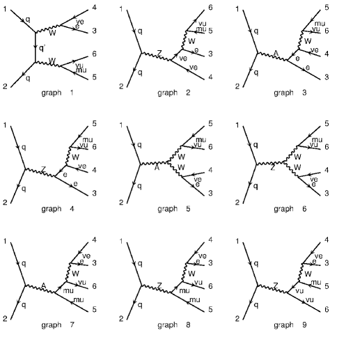
Figure 7: Topologies of Feynman diagrams for the process in eq. (1). Here the labels $Z$ and $W$ refer to all possible gauge boson states of the model, neutral and charged, respectively.

To calculate the cross section at the LHC for our model in the charged di-boson channel we consider three different set of cuts: a ‘standard cuts’ scenario, a ‘soft cuts’ scenario and a ‘hard cuts’ scenario.
Standard Cuts (St) (some are inspired by Ref. Moretti (1997)):

• $M_{ll}>180$ GeV (to avoid main SM contributions from the $Z$ and $WW$ peaks: notice that this cut is in fact hard-coded in our event generation)

• $|\eta_{l}|<3$ (this is a standard acceptance cut)

• $p_{T}(l)>20$ GeV (this is also a standard acceptance cut)

• $E_{T}^{\rm miss}>50$ GeV (see Fig. 8)

• $\cos\phi_{ll}^{T}<-0.5$ (see Fig. 9)

• $\cos\theta_{ll}<0$ (see Fig. 9)

where $M_{ll}^{2}=(p_{e}+p_{\mu})^{2}$ is the invariant mass of the couple of charged leptons, $\eta_{l}$ is the pseudo-rapidity of the charged leptons, $p_{T}(l)$ is the transverse momentum of the charged leptons, $E_{T}^{\rm miss}$ is the missing transverse energy, defined as $(E_{T}^{\rm miss})^{2}=(p_{T}(e)+p_{T}(\mu))^{2}=(p_{T}(\nu_{e})+p_{T}(\nu_{\mu}))^{2}$. Further, $\cos\phi_{ll}^{T}<-0.5$ is the cosine between the two leptons in the transverse plane whereas $\cos\theta_{ll}$ is the cosine between the two leptons. These are standard cuts, useful for a general purpose search.
Soft Cuts (So):

• $M_{ll}>180$ GeV

• $|\eta_{l}|<2$ (to exclude the regions where the difference with the SM is small)

• $p_{T}(l)>20$ GeV

• $E_{T}^{\rm miss}>50$ GeV

• $P_{T}^{\rm max}(l)>180$ GeV (see Fig. 8)

• $\cos\phi_{ll}^{T}<-0.5$

• $\cos\theta_{ll}<0$

where $P_{T}^{\rm max}(l)={\rm max}(P_{T}(e),P_{T}(\mu))$. These cuts are studied to further suppress the SM, leaving however not too small a signal cross section.
Hard Cuts (Ha):

• $M_{ll}>220$ GeV

• $|\eta_{l}|<1.5$

• $p_{T}(l)>20$ GeV

• $E_{T}^{\rm miss}>220$ GeV

• $P_{T}^{\rm max}>220$ GeV

• $\cos\phi_{ll}^{T}<-0.5$

• $\cos\theta_{ll}<0$

which represent a general tightening of (some of) the previous ones, at a further cost to the signal. We will be using one or more of such cut combinations to explore the parameter space of our model, via di-boson production, after the preliminary exercise of displaying typical cross sections (both inclusive and exclusive) for it. For the case of DY processes, we instead refer the reader to Refs. Accomando et al. (2012); Accomando et al. (2011c, a); Accomando et al. (2009, 2008).

III.3 Distributions

Before exploring the full parameter space it is useful to consider some total rates and differential distributions for process (1), in a such way to understand the relevant new contributions to the cross section. (Incidentally, we ought to notice at this point that process (2), despite giving fully inclusive production cross sections of order tens of fb at all energy stages of the CERN machine, after any of the above sets of cuts is applied, turns out to fall under observability limits for all considered luminosities, so that we neglect considering it further in our analysis.) In Fig. 8 we consider $M_{1}=1$ TeV and the maximal allowed value for $a_{W_{1}}$ for $z=0.8$ (see Fig. 3), and we display four relevant observables (we use the So cuts here). Herein, in order to better understand the role of the single neutral resonances in $s$-channel, we show also the contribution from the $Z_{1}$ and $Z_{2}$ resonances separately. It is quite clear that the second resonance ($Z_{2}$) is almost invisible and does not contribute to the total cross section. This is due to the fact that the trilinear gauge vertex ($Z_{2}WW$) is strongly suppressed due to the axial characteristics of the $Z_{2}$ state, so the only visible resonance is the lighter one. Remarkably, this is a completely different scenario from the DY one, in which the heavy state contribution to DY in both the Charged Current (CC) and Neutral Current (NC) case is the dominant one and often (especially in the former case) covers also the signal of the lighter one. This fact renders the di-boson channel a very valuable process to exploit in order to complement the scope of the DY one, so that both modes can be taken together to effectively cooperate in allowing one to see the typical multi-resonance structure of the gauge sector of the 4-site model. In addition to observables already introduced when defining the cuts, we also use the following additional ones:

$$P_{T}(\nu\nu)=\sqrt{p_{T}(e)^{2}+p_{T}(\mu)^{2}},\quad M_{T2}=p_{T}(e)+p_{T}(\mu)+E_{T}^{ll},$$ (29)

where

$$E_{T}^{ll}=p(e)^{0}+p(\mu)^{0},$$ (30)

which were not adopted for the final selections, yet they show some sizable differences between signal and background. In Fig. 9 we present the angular distributions used for our selection cuts, for the purpose of motivating the latter (the behaviour of the curves established towards the right end of the angular intervals plotted is maintained beyond it too). Finally, in Fig. 10 we show the same relevant observables of Fig. 8, considering three different mass scenarios (still for $z=0.8$), proving that they are generally effective independently of the mass values of the resonances.

Figure 8: Differential cross sections pertaining to the di-boson process for the 4-site model, for $M_{1}$=1 TeV and $z=0.8$. We choose the maximal not excluded value for $a_{W_{1}}$. Here, $P_{T}(\nu\nu)$ is the transverse momentum of two neutrinos in the transverse plane as defined in the text whereas $M_{T2}$ is the transverse mass as defined in Ref. Aad et al. (2012). The red-solid curve represents the full 4-site model, the green-dashed(blue-dotted) curve represents the $Z_{1}$($Z_{2}$) contribution alone and the black-dotted-dashed curve is the SM. So cuts were applied.

Figure 9: Differential cross sections pertaining to the di-boson process for the 4-site model, for $M_{1}$=1 TeV and $z=0.8$. We choose the maximal not excluded value for $a_{W_{1}}$. So cuts are applied. The red-solid curve represents the full 4-site model, the green-dashed(blue-dotted) curve represents the $Z_{1}$($Z_{2}$) contribution alone and the black-dotted-dashed curve is the SM. So cuts were applied.

Figure 10: Differential cross sections pertaining to the di-boson process for the 4-site model, for $M_{1}$=0.5, 1 and 1.5 TeV and $z=0.8$. We choose the maximal not excluded value for $a_{W_{1}}$. Some relevant distributions concerning the di-boson process for the 4-site model, for $M_{1}$=0.5 (red-solid), 1 (green-dashed), 1.5 (blue-dotted) TeV. The black-dot-dashed curve is the SM. All observables have been previously defined. So cuts are applied.

III.4 Exploring the parameter space

In this section we present some numerical values for the cross section at the LHC with, initially, 7 TeV, for some benchmark points in the parameter space, defined by five sets of masses for each one of the four chosen $z$ values. For each mass we consider the maximal allowed value for $a_{W_{1}}$. The mass values are $M_{1}=$0.5, 0.75, 1, 1.5 and 2 TeV for $z$ from 0.4 to 0.8. For $z=0.95$ the lower value for the mass is excluded, so we consider instead the scenario $M_{1}=1.7$ TeV. In Tabs. 2, 4, 6 and 8 we show the cross sections for such scenarios, for all our cut choices and including also a ‘No Cuts’ reference scenario (as defined in the captions). In Tabs. 3, 5, 7 and 9 we present instead the statistical significance $S$, defined as in eq. (27), considering a luminosity of 10 fb^-1. Here, we note that, for almost all masses and $z$ values considered, the So cuts allow for the largest statistical significances. Therefore, we decided to use the So cuts to explore the full parameter space of the 4-site model with larger data samples, in particular, we consider both the actual (8 TeV with 5 fb^-1) and future (8 and 14 TeV with 15 fb^-1) LHC scenarios. In Tabs. 10-13 are listed the ensuing cross sections and statistical significances.

$z=0.4$, $M_{1}$ [TeV]	No Cuts1 (10.5) [fb]	St (1.7) [fb]	So (0.58) [fb]	Ha (0.025) [fb]
0.5	21.2	6.09	3.16	0.17
0.75	16.7	5.14	3.66	0.39
1	13.7	3.84	2.61	0.52
1.5	11.2	2.55	1.78	0.30
2	10.7	1.83	0.74	0.12

Table 2: Cross section for the 4-site model considering the process of eq. (1) at the 7 TeV LHC for five different mass values and $z=0.4$. The values in parenthesis refer to the SM. ¹The only cut is on the invariant mass of the charged leptons and is set to 180 GeV.

$z=0.4$, $M_{1}$ [TeV]	No Cuts1	St	So	Ha
0.5	10.4	10.6	11.4	1.5
0.75	6.0	8.3	13.6	3.7
1	3.1	5.2	9.0	5.0
1.5	0.7	2.1	5.4	2.8
2	0.2	0.3	0.9	1.0

Table 3: Statistical significance ($S$) for the 4-site model considering the process of eq. (1) at the 7 TeV LHC for different mass values and $z=0.4$, for L=10 fb^-1. ¹The only cut is on the invariant mass of the charged leptons and is set to 180 GeV.

$z=0.6$, $M_{1}$ [TeV]	No Cuts1 (10.5) [fb]	St (1.7) [fb]	So (0.58) [fb]	Ha (0.025) [fb]
0.5	25.7	7.82	4.25	0.22
0.75	19.5	6.67	4.97	0.61
1	14.8	4.56	3.39	0.75
1.5	11.4	2.52	1.40	0.41
2	10.6	1.87	0.79	0.14

Table 4: Same as Tab. 2 for $z=0.6$.

$z=0.6$, $M_{1}$ [TeV]	No Cuts1	St	So	Ha
0.5	14.8	14.8	16.2	2.0
0.75	8.8	12.0	19.3	5.9
1	4.2	6.9	12.4	7.3
1.5	0.9	2.0	3.8	3.9
2	0.2	0.4	1.1	1.2

Table 5: Same as Tab. 3 for $z=0.6$.

$z=0.8$, $M_{1}$ [TeV]	No Cuts1 (10.5) [fb]	St (1.7) [fb]	So (0.58) [fb]	Ha (0.025) [fb]
0.5	23.7	6.85	3.78	0.22
1	15.2	4.69	3.55	0.87
1.5	12.1	2.97	1.91	0.68
1.7	11.4	2.51	1.38	0.48
2	10.7	2.03	0.91	0.23

Table 6: Same as Tab. 2 for $z=0.8$.

$z=0.8$, $M_{1}$ [TeV]	No Cuts1	St	So	Ha
0.5	12.9	12.5	14.1	2.0
1	4.6	7.2	13.1	8.5
1.5	1.6	3.1	6.0	6.6
1.7	0.9	2.0	3.7	4.6
2	0.2	0.8	1.6	2.1

Table 7: Same as Tab. 3 for $z=0.8$.

$z=0.95$, $M_{1}$ [TeV]	No Cuts1 (10.5) [fb]	St (1.7) [fb]	So (0.58) [fb]	Ha (0.025) [fb]
0.75	14.8	3.97	2.67	0.44
1	12.0	2.62	1.54	0.41
1.5	11.1	2.19	1.09	0.34
1.7	11.4	2.28	1.17	0.45
2	11.1	2.14	1.07	0.41

Table 8: Same as Tab. 2 for $z=0.95$.

$z=0.95$, $M_{1}$ [TeV]	No Cuts1	St	So	Ha
0.75	4.2	5.5	9.3	4.2
1	1.5	2.2	4.4	3.9
1.5	0.6	1.2	2.4	3.2
1.7	0.9	1.4	2.8	4.3
2	1.0	1.1	2.3	3.9

Table 9: Same as Tab. 3 for $z=0.95$.

$M_{1}$ [TeV]	0.5	0.75	1	1.5	1.7	2
$z=0.4$	4.15	4.08	3.58	1.7	1.31	1.00
$z=0.6$	5.53	6.89	5.24	2.36	1.62	1.15
$z=0.8$	4.73	5.32	4.72	2.9	2.21	1.43
$z=0.95$	-	3.56	2.06	1.6	1.83	1.74

Table 10: Cross sections (in [fb]) for the 4-site model considering the process of eq. (1) at the 8 TeV LHC for different mass and $z$ values. The value for the SM is 0.73 fb. We consider So cuts only.

$M_{1}$ [TeV]	0.5	0.75	1	1.5	1.7	2
$z=0.4$	15.5	15.2	12.9	4.4	2.6	1.2
$z=0.6$	21.8	27.9	20.4	7.4	3.9	1.9
$z=0.8$	18.1	20.8	18.1	9.8	6.7	3.2
$z=0.95$	12.8	12.8	6.0	3.9	5.0	4.6

Table 11: Statistical significance ($S$) for the 4-site model considering the process of eq. (1) at the 8 TeV LHC for different mass and $z$ values, for L=15 fb^-1. We consider So cuts only.

$M_{1}$ [TeV]	0.5	0.75	1	1.5	1.7	2
$z=0.4$	10.4	12.5	10.4	6.26	5.09	3.86
$z=0.6$	12.7	17.7	15.3	9.87	6.82	5.15
$z=0.8$	11.1	13.3	14.9	13.3	11.4	8.38
$z=0.95$	-	9.36	8.8	6.95	5.1	4.56

Table 12: Cross sections (in [fb]) for the 4-site model considering the process of eq. (1) at the 14 TeV LHC for different mass and $z$ values. The value for the SM is 1.55 fb. We consider the So cuts only.

$M_{1}$ [TeV]	0.5	0.75	1	1.5	1.7	2
$z=0.4$	22.5	27.8	22.5	12.0	9.0	5.9
$z=0.6$	28.3	41.0	34.9	21.1	13.4	9.1
$z=0.8$	24.3	29.8	33.9	29.8	25.0	17.3
$z=0.95$	-	19.8	18.4	13.7	9.02	7.6

Table 13: Statistical significance ($S$) for the 4-site model considering the process of eq. (1) at the 14 TeV LHC for different mass and $z$ values, for L=10 fb^-1. We consider So cuts only.

III.5 Exclusion and discovery bounds

In this section we compute the actual bounds from the LHC on the 4-site model in considering di-boson production, and we contrast them to the corresponding figures obtained via (both CC and NC) DY processes. As explained before, we apply the efficiency on reconstructing the two charged leptons as extracted from the DY channels, supplemented by an additional efficiency on the missing energy, and we remind the reader that we made this choice because at present there are no published di-boson analyses on possible extra gauge boson pairs. For reference, first we take the current experimental limits as obtained from DY processes (as per previous figures, hereafter labelled as ‘DY 5 fb^-1 in the plots). Then, we consider the limits from the following LHC setups assuming di-boson production and decay: 7 TeV with 5 fb^-1, 8 TeV with 15 fb^-1 and 14 TeV with 15 fb^-1. As before, we consider four representative values of the $z$ parameter. The results for the exclusion areas are showed in Fig. 11 whilst those for the discovery regions are found in Fig. 12. As we can see from these figures, a large part of the parameter space will be explored from the LHC in the next few years, excluding or discovering the 4-site model, using the di-boson channel alone.

Finally, in Fig. 13 we perform a comparison (using the aforementioned efficiencies) between the di-boson and the DY channels, in exclusion limits only, for the LHC at 8 and 14 TeV, both with 15 fb^-1, for two significant values of $z$. The result is that the di-boson mode is more efficient, both at low and high values of the $W_{1}$ mass, with respect to the DY channels, and this is due to the fact that the trilinear vertex $Z_{1}WW$ is of the same magnitude as the SM coupling $ZWW$ and, moreover, upon the couplings to the fermions, but only on $z$ and $M_{1}$, so that the di-boson mode can help exploring also the low coupling region. As we can see from these figures, except for the region of very small $a_{W_{1}}$ couplings and masses above 1 TeV, the rest of the parameter space which has survived experimental constraints will be explored from the LHC in the next few years, excluding or discovering the 4-site model, by synergistically exploiting both the DY and di-boson channels.

In closing, we should also emphasise that, for reason of space, we have illustrated the scope of DY and di-boson production and decay in setting bounds on our model only limitedly to the case of the charged sector, i.e., over the ($M_{W_{1}}$, $\alpha_{W_{1}}$) plane. We can however confirm that a similar pattern can be established in the case of the neutral one as well. i.e., over the ($M_{Z_{1}}$, $\alpha_{Z_{1}}^{L}(l)$) plane.

Figure 11: Shown are the 95% CL exclusion limits from the LHC on the 4-site model: here, we consider the di-boson channel for the usual four values of the $z$ parameter. We assume all possible LHC setups considered.

Figure 12: Shown are the $5\sigma$ discovery limits from the LHC on the 4-site model: here, we consider the di-boson channel for the usual four values of the $z$ parameter. We assume all possible LHC setups considered.

Figure 13: Shown are the 95% CL exclusion limits from the LHC on the 4-site model: here, we consider both the DY (blue-dashed line) and di-boson (green-dot-dashed line) channels for two values of the $z$ parameter. We assume only the LHC setups at 8 and 14 TeV with 15 fb^-1.

IV Summary and conclusions

In summary, we have studied the scope of the various LHC stages in testing the parameter space of a 4-site model of strong EWSB supplemented with the presence of one composite Higgs boson, compatible with the most recent experimental limits from both EWPTs and direct searches for new Higgs and gauge boson resonances as well as compliant with theoretical requirements of unitarity. We have done so by exploiting a process so far largely neglected in experimental analyses, i.e., charged di-boson production into two opposite-charge different-flavour leptons, namely, $e^{\pm}\mu^{\mp}E_{T}^{\rm miss}$ final states, where the keyword ‘charged’ refers to the intermediate stage of charged $W$-boson pairs being produced in all combinations possible in our scenario. We then contrasted the yield of this mode with results obtained from both CC and NC DY processes. In both cases we exploited dedicated parton-level analyses based on acceptance and selection cuts specifically designed to exalt the complementary role that these two channels can have at the CERN machine in constraining or revealing our EWSB scenario. Specifically, we have come to the following key conclusions.

• DY channels are mostly sensitive to the second gauge boson resonance ($W_{2}$ in CC and $Z_{2}$ in NC) whilst charged di-boson production is mostly sensitive to the lightest states, i.e., $W_{1}$ and $Z_{1}$, all produced in resonant topologies occurring in either subprocess. Therefore, the exploitation of this synergy will eventually enable one to elucidate the full gauge boson spectrum and its dynamics in the context of our scenario.

• The di-boson channel, which is entirely new to this study, further offers an advantage over the DY modes, in the sense that it enables one to explore small couplings of the new gauge bosons to the SM fermions, in virtue of the fact that the overall rate of this process is dependent upon trilinear gauge boson self-couplings which can be very large per se and are further onset in resonant topologies.

Benchmark points of the model under consideration amenable to phenomenogical investigation have been defined and their efficacy in probing different regions of parameter space was emphasised by adopting all past, current and future setups of the CERN machine.

Finally, a set of numerical tools enabling the accurate prediction of the model spectrum as well as the fast event generation (of both signal and background) in fully differential form have been produced and are available upon request.

References

- Contino et al. (2010) R. Contino, C. Grojean, M. Moretti, F. Piccinini, and R. Rattazzi, JHEP 1005, 089 (2010), eprint 1002.1011.
- Espinosa et al. (2012a) J. Espinosa, C. Grojean, M. Muhlleitner, and M. Trott, JHEP 1205, 097 (2012a), eprint 1202.3697.
- Bellazzini et al. (2012) B. Bellazzini, C. Csaki, J. Hubisz, J. Serra, and J. Terning (2012), eprint 1205.4032.
- Gillioz et al. (2012) M. Gillioz, R. Grober, C. Grojean, M. Muhlleitner, and E. Salvioni (2012), eprint 1206.7120.
- Agashe et al. (2003) K. Agashe, A. Delgado, M. J. May, and R. Sundrum, JHEP 08, 050 (2003), eprint hep-ph/0308036.
- Csaki et al. (2004a) C. Csaki, C. Grojean, H. Murayama, L. Pilo, and J. Terning, Phys. Rev. D69, 055006 (2004a), eprint hep-ph/0305237.
- Csaki et al. (2004b) C. Csaki, C. Grojean, L. Pilo, and J. Terning, Phys. Rev. Lett. 92, 101802 (2004b), eprint hep-ph/0308038.
- Barbieri et al. (2004) R. Barbieri, A. Pomarol, and R. Rattazzi, Phys. Lett. B591, 141 (2004), eprint hep-ph/0310285.
- Cacciapaglia et al. (2004a) G. Cacciapaglia, C. Csaki, C. Grojean, and J. Terning, ECONF C040802, FRT004 (2004a).
- Cacciapaglia et al. (2004b) G. Cacciapaglia, C. Csaki, C. Grojean, and J. Terning, Phys. Rev. D70, 075014 (2004b), eprint hep-ph/0401160.
- Arkani-Hamed et al. (2001a) N. Arkani-Hamed, A. G. Cohen, and H. Georgi, Phys. Rev. Lett. 86, 4757 (2001a), eprint hep-th/0104005.
- Arkani-Hamed et al. (2001b) N. Arkani-Hamed, A. G. Cohen, and H. Georgi, Phys. Lett. B513, 232 (2001b), eprint hep-ph/0105239.
- Hill et al. (2001) C. T. Hill, S. Pokorski, and J. Wang, Phys. Rev. D64, 105005 (2001), eprint hep-th/0104035.
- Cheng et al. (2001) H.-C. Cheng, C. T. Hill, S. Pokorski, and J. Wang, Phys. Rev. D64, 065007 (2001), eprint hep-th/0104179.
- Abe et al. (2003) H. Abe, T. Kobayashi, N. Maru, and K. Yoshioka, Phys. Rev. D67, 045019 (2003), eprint hep-ph/0205344.
- Falkowski and Kim (2002) A. Falkowski and H. D. Kim, JHEP 08, 052 (2002), eprint hep-ph/0208058.
- Randall et al. (2003) L. Randall, Y. Shadmi, and N. Weiner, JHEP 01, 055 (2003), eprint hep-th/0208120.
- Son and Stephanov (2004) D. T. Son and M. A. Stephanov, Phys. Rev. D69, 065020 (2004), eprint hep-ph/0304182.
- de Blas et al. (2006) J. de Blas, A. Falkowski, M. Perez-Victoria, and S. Pokorski, JHEP 08, 061 (2006), eprint hep-th/0605150.
- Chivukula et al. (2006) R. S. Chivukula et al., Phys. Rev. D74, 075011 (2006), eprint hep-ph/0607124.
- Accomando et al. (2009) E. Accomando, S. De Curtis, D. Dominici, and L. Fedeli, Phys. Rev. D79, 055020 (2009), eprint 0807.5051.
- Contino et al. (2007) R. Contino, T. Kramer, M. Son, and R. Sundrum, JHEP 05, 074 (2007), eprint hep-ph/0612180.
- Incandela (July 4, 2012) J. Incandela, CMS talk at Latest update in the search for the Higgs boson at CERN (July 4, 2012), eprint http://indico.cern.ch/conferenceDisplay.py?confId=197461.
- Gianotti (July 4, 2012) F. Gianotti, ATLAS talk at Latest update in the search for the Higgs boson at CERN (July 4, 2012), eprint http://indico.cern.ch/conferenceDisplay.py?confId=197461.
- Accomando et al. (2011a) E. Accomando, S. De Curtis, D. Dominici, and L. Fedeli, Phys. Rev. D83, 015012 (2011a), eprint 1010.0171.
- Accomando et al. (2011b) E. Accomando, D. Becciolini, L. Fedeli, D. Dominici, and S. De Curtis, Phys. Rev. D83, 115021 (2011b), eprint 1105.3896.
- Accomando et al. (2011c) E. Accomando, D. Becciolini, S. De Curtis, D. Dominici, and L. Fedeli, Phys. Rev. D84, 115014 (2011c), eprint 1107.4087.
- Accomando et al. (2012) E. Accomando, D. Becciolini, S. De Curtis, D. Dominici, L. Fedeli, et al., Phys. Rev. D85, 115017 (2012), eprint 1110.0713.
- Casalbuoni et al. (1989) R. Casalbuoni, S. De Curtis, D. Dominici, F. Feruglio, and R. Gatto, Int. J. Mod. Phys. A4, 1065 (1989).
- Coleman et al. (1969) S. R. Coleman, J. Wess, and B. Zumino, Phys. Rev. 177, 2239 (1969).
- Callan et al. (1969) J. Callan, Curtis G., S. R. Coleman, J. Wess, and B. Zumino, Phys. Rev. 177, 2247 (1969).
- Bando et al. (1988) M. Bando, T. Kugo, and K. Yamawaki, Phys.Rept. 164, 217 (1988).
- Casalbuoni et al. (2004) R. Casalbuoni, S. De Curtis, and D. Dominici, Phys. Rev. D70, 055010 (2004), eprint hep-ph/0405188.
- Casalbuoni et al. (1997) R. Casalbuoni, S. De Curtis, and D. Dominici, Phys. Lett. B403, 86 (1997), eprint hep-ph/9702357.
- Casalbuoni et al. (1996) R. Casalbuoni, S. De Curtis, D. Dominici, and M. Grazzini, Phys. Lett. B388, 112 (1996), eprint hep-ph/9607276.
- Accomando et al. (2008) E. Accomando, S. De Curtis, D. Dominici, and L. Fedeli, Nuovo Cim. 123B, 809 (2008), eprint 0807.2951.
- Peskin and Takeuchi (1990) M. E. Peskin and T. Takeuchi, Phys. Rev. Lett. 65, 964 (1990).
- Peskin and Takeuchi (1992) M. E. Peskin and T. Takeuchi, Phys. Rev. D46, 381 (1992).
- Altarelli and Barbieri (1991) G. Altarelli and R. Barbieri, Phys. Lett. B253, 161 (1991).
- Altarelli et al. (1998) G. Altarelli, R. Barbieri, and F. Caravaglios, Int. J. Mod. Phys. A13, 1031 (1998), eprint hep-ph/9712368.
- Gunion (2012) J. Gunion, talk at LPCC workshop Implications of LHC results for the TeV physics (2012).
- Gunion et al. (2012) J. F. Gunion, Y. Jiang, and S. Kraml (2012), eprint 1207.1545.
- Azatov et al. (2012) A. Azatov, R. Contino, and J. Galloway (2012), eprint 1206.3171.
- Ellis and You (2012) J. Ellis and T. You (2012), eprint 1207.1693.
- Espinosa et al. (2012b) J. Espinosa, C. Grojean, M. Muhlleitner, and M. Trott (2012b), eprint 1207.1717.
- Petrucciani (2012) G. Petrucciani, talk at LPCC workshop Implications of LHC results for the TeV physics (2012).
- Giardino et al. (2012) P. P. Giardino, K. Kannike, M. Raidal, and A. Strumia (2012), eprint 1207.1347.
- Chatrchyan et al. (2012) S. Chatrchyan et al. (CMS Collaboration) (2012), eprint 1204.4764.
- Chatrchyan et al. (2011) S. Chatrchyan et al. (CMS Collaboration), JINST 6, P09001 (2011), eprint 1106.5048.
- Belyaev et al. (2009) A. Belyaev et al., Phys. Rev. D79, 035006 (2009), eprint 0809.0793.
- Ballestrero (1999) A. Ballestrero (1999), eprint hep-ph/9911318.
- Murayama et al. (1992) H. Murayama, I. Watanabe, and K. Hagiwara (1992), eprint KEK-91-11.
- Stelzer and Long (1994) T. Stelzer and W. Long, Comput. Phys. Commun. 81, 357 (1994), eprint hep-ph/9401258.
- Kunszt et al. (1997) Z. Kunszt, S. Moretti, and W. J. Stirling, Z.Phys. C74, 479 (1997), eprint hep-ph/9611397.
- Kleiss et al. (1986) R. Kleiss, W. J. Stirling, and S. Ellis, Comput. Phys. Commun. 40, 359 (1986).
- Lepage (1978) G. P. Lepage, J. Comput. Phys. 27, 192 (1978).
- Lai et al. (2000) H. Lai et al. (CTEQ Collaboration), Eur. Phys. J. C12, 375 (2000), eprint hep-ph/9903282.
- Moretti (1997) S. Moretti, Phys. Rev. D56, 7427 (1997), eprint hep-ph/9705388.
- Aad et al. (2012) G. Aad et al. (ATLAS Collaboration), Phys. Lett. B712, 289 (2012), eprint 1203.6232.