Classical double-well systems coupled to finite baths

Abstract

We have studied properties of a classical $N_{S}$-body double-well system coupled to an $N_{B}$-body bath, performing simulations of $2(N_{S}+N_{B})$ first-order differential equations with $N_{S}\simeq 1-10$ and $N_{B}\simeq 1-1000$. A motion of Brownian particles in the absence of external forces becomes chaotic for appropriate model parameters such as $N_{B}$, $c_{o}$ (coupling strength), and $\{\omega_{n}\}$ (oscillator frequency of bath): For example, it is chaotic for a small $N_{B}$ ($\lesssim 100$) but regular for a large $N_{B}$ ($\gtrsim 500$). Detailed calculations of the stationary energy distribution of the system $f_{S}(u)$ ($u$: an energy per particle in the system) have shown that its properties are mainly determined by $N_{S}$, $c_{o}$ and $T$ (temperature) but weakly depend on $N_{B}$ and $\{\omega_{n}\}$. The calculated $f_{S}(u)$ is analyzed with the use of the $\Gamma$ distribution. Difference and similarity between properties of double-well and harmonic-oscillator systems coupled to finite bath are discussed.

I Introduction

Many studies have been made with the use of a model describing a classical or quantum open system which is coupled to baths consisting of a collection of harmonic oscillators. Such a model is conventionally referred to as the Caldeira-Leggett (CL) model Caldeira81 ; Caldeira83 , although equivalent models had been proposed earlier by Magalinskii Magalinskii59 and Ullersma Ullersma66 . From the CL model, we may derive the Langevin model with dissipation and diffusion (noise) terms. Originally the CL model was introduced for $N_{B}$-body bath with $N_{B}\rightarrow\infty$, for which the Ohmic and Drude-type spectral densities with continuous distributions are adopted. Furthermore in the original CL model, the number of particles in a systems, $N_{S}$, is taken to be unity ($N_{S}=1$). We expect that a generic open system may contain any number of particles and that a system may be coupled to a bath consisting of finite harmonic oscillators in general. In recent years, the CL model has been employed for a study of properties of open systems with finite $N_{S}$ and/or $N_{B}$ Smith08 ; Wei09 ; Hanggi08 ; Ingold09 ; Rosa08 ; Hasegawa11 ; Carcaterra11 ; Hasegawa11c ; Hasegawa11b . Specific heat anomalies of quantum oscillator (system) coupled to finite bath have been studied Hanggi08 ; Ingold09 ; Hasegawa11c . A thermalization Smith08 ; Wei09 , energy exchange Rosa08 , dissipation Carcaterra11 and the Jarzynski equality Jarzynski97 ; Hasegawa11b in classical systems coupled to finite bath have been investigated.

In a previous paper Hasegawa11 , we have studied the $(N_{S}+N_{B})$ model for finite $N_{S}$-body systems coupled to baths consisting of $N_{B}$ harmonic oscillators. Our study for open harmonic oscillator systems with $N_{S}\simeq 1-10$ and $N_{B}\simeq 10-1000$ has shown that stationary energy distribution of the system has a significant and peculiar dependence on $N_{S}$, but it weakly depends on $N_{B}$ Hasegawa11 . These studies mentioned above Smith08 ; Wei09 ; Hanggi08 ; Ingold09 ; Rosa08 ; Hasegawa11 ; Carcaterra11 ; Hasegawa11c ; Hasegawa11b have been made for harmonic-oscillator systems with finite $N_{S}$ and/or $N_{B}$.

Double-well potential models have been employed in a wide range of fields including physics, chemistry and biology (for a recent review on double-well system, see Ref. Thorwart01 ). Various phenomena such as the stochastic resonance (SR), tunneling through potential barrier and thermodynamical properties Hasegawa12b have been studied. The CL model for the double-well systems with $N_{S}=1$ and $N_{B}=\infty$ has been extensively employed for a study on the SR Gamma98 . Properties of SR for variations of magnitude of white noise Hanggi84 ; Hanggi93 ; Gamma89 ; Gamma98 and relaxation time of colored noise Neiman96 ; Hasegawa12 have been studied. However, studies for open double-well systems with finite $N_{S}$ and/or $N_{B}$ have not been reported as far as we are aware of. It would be interesting and worthwhile to study open classical double-well systems described by the $(N_{S}+N_{B})$ model with finite $N_{S}$ and $N_{B}$, which is the purpose of the present paper.

The paper is organized as follows. In Sec. II, we briefly explain the $(N_{S}+N_{B})$ model proposed in our previous study Hasegawa11 . In Sec. III, direct simulations (DSs) of $2(N_{S}+N_{B})$ first-order differential equations for the adopted model have been performed. Dynamics of a single double-well system ($N_{S}=1$) coupled to a finite bath ($2\leq N_{B}\leq 1000$) in the phase space is investigated (Sec. III B). We study stationary energy distributions in the system and bath, performing detailed DS calculations, changing $N_{S}$, $N_{B}$, the coupling strength and the distribution of bath oscillators (Sec. III C). Stationary energy and position distributions obtained by DSs are analyzed in Sec. IV. The final Sec. V is devoted to our conclusion.

II Adopted ($N_{S}+N_{B}$) model

We consider a system including $N_{S}$ Brownian particles coupled to a bath consisting of independent $N_{B}$ harmonic oscillators. We assume that the total Hamiltonian is given by Hasegawa11

$$H = H_{S}+H_{B}+H_{I},$$ (1)

with

$$H_{S} = \sum_{k=1}^{N_{S}}\left[\frac{P_{k}^{2}}{2M}+V(Q_{k})\right],$$ (2)

$$H_{B} = \sum_{n=1}^{N_{B}}\left[\frac{p_{n}^{2}}{2m}+\frac{m\omega_{n}^{2}}{2}q_{n}^{2}\right],$$ (3)

$$H_{I} = \frac{1}{2}\sum_{k=1}^{N_{S}}\sum_{n=1}^{N_{B}}c_{kn}(Q_{k}-q_{n})^{2},$$ (4)

where $H_{S}$, $H_{B}$ and $H_{I}$ express Hamiltonians for the system, bath and interaction, respectively. Here $M$ ($m$) denotes the mass, $P_{k}$ ($p_{n}$) the momentum, $Q_{k}$ ($q_{n}$) position of the oscillator in the system (bath), $V(Q_{k})$ signifies the potential in the system, $\omega_{n}$ stands for oscillator frequency in the bath, and $c_{nk}$ is coupling constant. The model is symmetric with respect to an exchange of system $\leftrightarrow$ bath if $V(Q)$ is the harmonic potential. From Eqs. (1)-(4), we obtain $2(N_{S}+N_{B})$ first-order differential equations,

$$\dot{Q}_{k} = \frac{P_{k}}{M},$$ (5)

$$\dot{P}_{k} = -V^{\prime}(Q_{k})-\sum_{n=1}^{N_{B}}c_{kn}(Q_{k}-q_{n}),$$ (6)

$$\dot{q}_{n} = \frac{p_{n}}{m},$$ (7)

$$\dot{p}_{n} = -m\omega_{n}^{2}q_{n}-\sum_{k=1}^{N_{S}}c_{kn}(q_{n}-Q_{k}),$$ (8)

which yield

$$M\ddot{Q}_{k} = -V^{\prime}(Q_{k})-\sum_{n=1}^{N_{B}}c_{kn}(Q_{k}-q_{n}),$$ (9)

$$m\ddot{q}_{n} = -m\omega_{n}^{2}q_{n}-\sum_{k=1}^{N_{S}}c_{kn}(q_{n}-Q_{k}),$$ (10)

with prime (^′) and dot ($\cdot$) denoting derivatives with respect to the argument and time, respectively. It is noted that the second term of Eq. (6) or (9) given by

$$F_{k}^{(eff)} = -\sum_{n=1}^{N_{B}}c_{kn}(Q_{k}-q_{n}),$$ (11)

plays a role of the effective force to the $k$th system.

A formal solution of Eq. (10) for $q_{n}(t)$ is given by

$$q_{n}(t) = q_{n}(0)\cos\tilde{\omega}_{n}t+\frac{\dot{q}_{n}(0)}{\tilde{\omega}_{n}}\sin\tilde{\omega}_{n}t+\sum_{\ell=1}^{N_{S}}\frac{c_{\ell n}}{m\tilde{\omega}_{n}}\int_{0}^{t}\sin\tilde{\omega}_{n}(t-t^{\prime})Q_{\ell}(t^{\prime})\>dt^{\prime},$$ (12)

with

$$\tilde{\omega}_{n}^{2} = \frac{b_{n}}{m}+\sum_{k=1}^{N_{S}}\frac{c_{kn}}{m}=\omega_{n}^{2}+\sum_{k=1}^{N_{S}}\frac{c_{kn}}{m}.$$ (13)

Substituting Eq. (12) to Eq. (9), we obtain the non-Markovian Langevin equation given by

$$M\ddot{Q}_{k}(t) = -V^{\prime}(Q_{k})-M\sum_{\ell=1}^{N_{S}}\xi_{k\ell}Q_{\ell}(t)-\sum_{\ell=1}^{N_{S}}\int_{0}^{t}\gamma_{k\ell}(t-t^{\prime})\dot{Q}_{\ell}(t^{\prime})\>dt^{\prime}$$ (14)

$$- \sum_{\ell=1}^{N_{S}}\gamma_{k\ell}(t)Q_{\ell}(0)+\zeta_{k}(t)\hskip 28.45274pt\mbox{($k=1$ to $N_{S}$)},$$

with

$$M\xi_{k\ell} = \sum_{n=1}^{N_{B}}\left[c_{kn}\delta_{k\ell}-\frac{c_{kn}c_{\ell n}}{m\tilde{\omega}_{n}^{2}}\right],$$ (15)

$$\gamma_{k\ell}(t) = \sum_{n=1}^{N_{B}}\left(\frac{c_{kn}c_{\ell n}}{m\tilde{\omega}_{n}^{2}}\right)\cos\tilde{\omega}_{n}t,$$ (16)

$$\zeta_{k}(t) = \sum_{n=1}^{N_{B}}c_{kn}\left[q_{n}(0)\cos\tilde{\omega}_{n}t+\frac{\dot{q}_{n}(o)}{\tilde{\omega}_{n}}\sin\tilde{\omega}_{n}t\right],$$ (17)

where $\xi_{k\ell}$ denotes the additional interaction between $k$ and $\ell$th particles in the system induced by couplings $\{c_{kn}\}$, $\gamma_{k\ell}(t)$ the memory kernel and $\zeta_{k}$ the stochastic force.

If the equipartition relation is realized in initial values of $q_{n}(0)$ and $\dot{q}(0)$,

$$\langle m\tilde{\omega}_{n}^{2}q_{n}(0)^{2}\rangle_{B} = \langle m\dot{q}_{n}(0)^{2}\rangle_{B}=k_{B}T,$$ (18)

we obtain the fluctuation-dissipation relation:

$$\langle\zeta_{k}(t)\zeta_{k}(t^{\prime})\rangle_{B} = k_{B}T\gamma_{kk}(t-t^{\prime}),$$ (19)

where $\langle\cdot\rangle_{B}$ stands for the average over variables in the bath.

In the case of $N_{B}\rightarrow\infty$, summations in Eqs. (15)-(17) are replaced by integrals. When the spectral density defined by

$$J(\omega)=\frac{\pi}{2}\sum_{n}\frac{c_{n}^{2}}{m_{n}\omega_{n}^{2}}\delta(\omega-\omega_{n}),$$ (20)

is given by the Ohmic form: $J(\omega)\propto\omega$ for $0\leq\omega<w_{D}$, the kernel becomes

$$\gamma(t)\propto\frac{\sin\omega_{D}t}{\pi t}\propto\delta(t),$$ (21)

which leads to the Markovian Langevin equation.

In the case of $N_{S}=1$, we obtain $\xi$ and $\gamma$ in Eqs. (15) and (16) where the subscripts $k$ and $\ell$ are dropped (e.g., $c_{kn}=c_{n}$),

$$M\xi(t) = \sum_{n=1}^{N_{B}}c_{n}\left(1-\frac{c_{n}}{m\tilde{\omega}_{n}^{2}}\right),$$ (22)

$$\gamma(t) = \sum_{n=1}^{N_{B}}\left(\frac{c_{n}^{2}}{m\tilde{\omega}_{n}^{2}}\right)\cos\tilde{\omega}_{n}t.$$ (23)

The additional interaction vanishes ($\xi=0$) if we choose $c_{n}=m\tilde{\omega}_{n}^{2}$ in Eq. (22).

In the case of $N_{S}\neq 1$, however, it is impossible to choose $\{c_{kn}\}$ such that $\xi_{k\ell}=0$ is realized for all pairs of $(k,\ell)$ in Eq. (15). Then $Q_{k}$ is inevitably coupled to $Q_{\ell}$ for $\ell\neq k$ with the superexchange-type interaction of antiferromagnets: $-\sum_{n}c_{kn}c_{\ell n}/m\tilde{\omega}_{n}^{2}$ in Eq. (15).

III Model calculations for double-well systems

III.1 Calculation methods

We consider a system with the double-well potential

$$V(Q) = \left(\frac{\Delta}{Q_{0}^{4}}\right)(Q^{2}-Q_{0}^{2})^{2},$$ (24)

which has the stable minima of $V(\pm Q_{0})=0$ at $Q=\pm Q_{0}$ and locally unstable maximum of $V(0)=\Delta$ at $Q=0$ with the barrier height $\Delta$. We have adopted $Q_{0}=1.0$ and $\Delta=1.0$ in our DSs.

It is easier to solve $2(N_{S}+N_{B})$ first-order differential equations given by Eqs. (5)-(8) than to solve the $N_{S}$ Langevin equations given by Eqs. (14)-(17) although the latter provides us with clearer physical insight than the former. In order to study the $N_{S}$ and $N_{B}$ dependences of various physical quantities, we have assumed that the coupling $c_{kn}$ is given by Hasegawa11 ; Note2

$$c_{kn}=\frac{c_{o}}{N_{S}N_{B}},$$ (25)

because the interaction term includes summations of $\sum_{k=1}^{N_{S}}$ and $\sum_{n=1}^{N_{B}}$ in Eq. (4). It is noted that with our choice of $c_{kn}$, the interaction contribution is finite even in the thermodynamical limit of $N_{B}\rightarrow\infty$ because the summation over $n$ runs from 1 to $N_{B}$ in Eq. (4). DSs of Eqs. (5)-(8) have been performed with the use of the fourth-order Runge-Kutta method with the time step of 0.01. We have adopted $k_{B}=1.0$, $M=m=1.0$, $c_{o}=1.0$, and $\omega_{n}=1.0$ otherwise noticed.

We consider energies per particle $u_{\eta}(t)$ in the system ($\eta$=S) and the bath ($\eta$=B) which are assume to be given by

$$u_{S} = \frac{1}{N_{S}}\sum_{k=1}^{N_{S}}\left[\frac{P_{k}^{2}}{2M}+V(Q_{k})\right],$$ (26)

$$u_{B} = \frac{1}{N_{B}}\sum_{n=1}^{N_{B}}\left[\frac{p_{n}^{2}}{2m}+\frac{m\omega_{n}^{2}q_{n}^{2}}{2}\right],$$ (27)

which is valid for the weak interaction, although a treatment of the finite interaction is ambiguous and controversial Hanggi08 ; Ingold09 .

III.2 Dynamics of a particle in the $(Q,P)$ phase space

III.2.1 Effect of $c_{o}$

First we consider an isolated double-well system ($N_{S}=1$ and $c_{o}=0.0$). Figure 1 shows the phase-space trajectories in the $(Q,P)$ phase space for this system with six different initial system energies $E_{So}$. For $E_{So}=0.0$, the system has two stable fixed points at $(Q,P)=(\pm 1.0,0.0)$, and for $E_{So}=\Delta=1.0$ it has one unstable fixed point at $(Q,P)=(0.0,0.0)$. In the case of $0.0<E_{So}<1.0$, the trajectory is restricted in the region of $Q>0.0$ (or $Q<0.0$). In contrast in the case of $E_{So}>1.0$, trajectory may visit both regions of $Q>0.0$ and $Q<0.0$. The case of $E_{So}=1.0$ is critical between the two cases.

Figure 1: Plot of phase-space trajectories for a particle in an isolated double-well system ($c_{o}=0.0$). Trajectories are plotted for energies of $E_{So}/\Delta=0.0$, 0.5, 0.8, 1.0, 1.2 and 1.5.

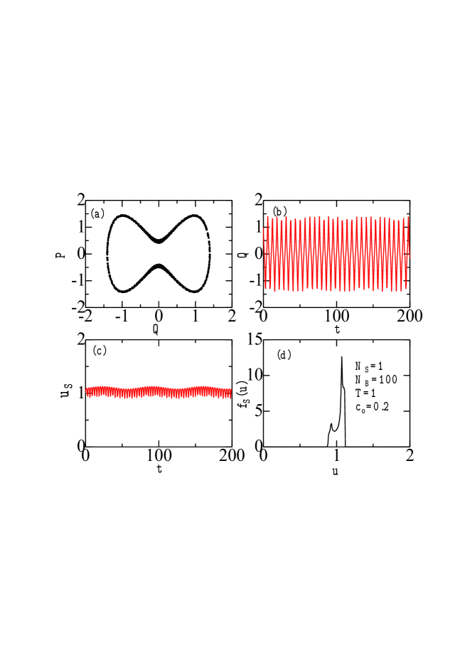
Figure 2: (Color online) (a) Strobe plot in the $(Q,P)$ phase space (with a time interval of 1.0), (b) $Q(t)$, (c) $u_{S}(t)$, and (d) the system energy distribution $f_{S}(u)$ obtained by a single run for $E_{So}=1.0$, $N_{S}=1$, $N_{B}=100$, $T=1.0$ and $c_{o}=0.2$.

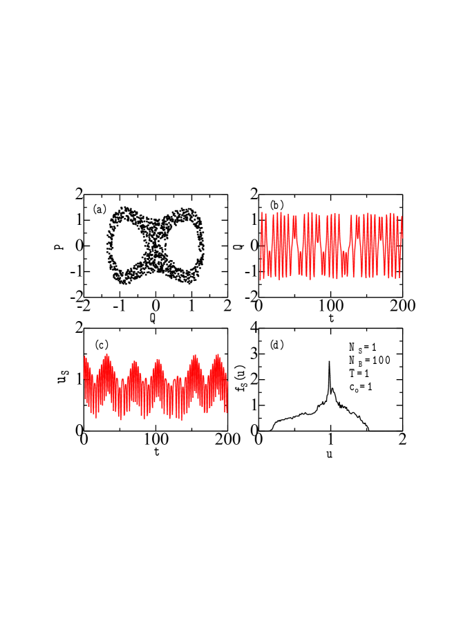
Figure 3: (Color online) (a) Strobe plot in the $(Q,P)$ phase space, (b) $Q(t)$, (c) $u_{S}(t)$, and (d) the system energy distribution $f_{S}(u)$ obtained by a single run for $E_{So}=1.0$, $N_{S}=1$, $N_{B}=100$, $T=1.0$ and $c_{o}=1.0$.

Next the double-well system is coupled to a bath. In our DSs, we have assumed that system and bath are decoupled at $t<0$ where they are in equilibrium states with $E_{So}=T$, the temperature $T$ being defined by $T=u_{B}$. We have chosen initial values of $Q(0)=1.0$ and $P(0)=\sqrt{2M[E_{So}-V(Q(0))]}$ for a given initial system energy $E_{So}$. Initial conditions for $q_{n}(0)$ and $p_{n}(0)$ are given by random Gaussian variables with zero means and variance proportional to $T$ [Eq. (18)] Hasegawa11 . Results to be reported in this subsection have been obtained by single runs for $t=0$ to 1000.

Figures 2(a) and 2(b) show a strobe plot in the $(Q,P)$ phase space (with a time interval of 1.0) and the time-dependence of $Q(t)$, respectively, for $E_{So}=1.0$, $N_{S}=1$, $N_{B}=100$ and $c_{o}=0.2$. The trajectory starting from $Q(0)=1.0$ goes to the negative-$Q$ region because a particle may go over the potential barrier with a help of a force (noise) originating from bath given by Eq. (11). The system energy fluctuates as shown in Fig. 2(c), whose distribution is plotted in Fig. 2(d).

Results in Fig. 2 are regular. In contrast, when a coupling strength is increased to $c_{o}=1.0$, the system becomes chaotic as shown in Figs. 3(a) and 3(b) where a strobe plot in the $(Q,P)$ phase space and the time-dependence of $Q(t)$ are plotted, respectively. This is essentially the force-induced chaos in classical double-well system Reichl84 : although an external force is not applied to our system, a force arising from a coupling with bath given by Eq. (11) plays a role of an effective external force for the system. Figures 3(c) and 3(d) show that in the case of $c_{o}=1.0$, $u_{S}$ has more appreciable temporal fluctuations with a wider energy distribution in $f_{S}(u)$ than in the case of $c_{o}=0.2$. Although system energies fluctuate, they are not dissipative at $0.0\leq t<1000.0$ in DSs both for $c_{o}=0.2$ and $c_{o}=1.0$ with $N_{B}=100$.

III.2.2 Effect of $\omega_{n}$ distributions

We have so far assumed $\omega_{n}=1.0$ in the bath, which is now changed. Figures 4(a) and 4(c) show strobe plots for $\omega_{n}=0.5$ and $2.0$, respectively, which are regular and which are different from a chaotic result for $\omega_{n}=1.0$ shown in Fig. 4(b). When we adopt $\{\omega_{n}\}$ which is randomly distributed in $[0.5,2.0]$, a motion of a system particle becomes chaotic as shown in Fig. 4(d). This is because contributions from $\omega_{n}\sim 1.0$ among $[0.5.2.0]$ induce chaotic behavior.

Figure 4: Strobe plots in the $(Q,P)$ phase space for various distribution of $\{\omega_{n}\}$: (a) $\omega_{n}=0.5$, (b) $\omega_{n}=1.0$, (c) $\omega_{n}=2.0$ and (d) $\omega_{n}\in[0.5,2.0]$ obtained by single runs with $E_{So}=1.0$, $N_{S}=1$, $N_{B}=100$, $T=1.0$ and $c_{o}=1.0$.

III.2.3 Effect of $N_{B}$

We have repeated calculations by changing $N_{B}$, whose results are plotted in Figs. 5(a)-5(d). Figures 5(a), 5(b) and 5(c) show that chaotic behaviors for $N_{B}=2$ and $N_{B}=10$ are more significant than that for $N_{B}=100$. On the contrary, chaotic behavior is not realized for $N_{B}=1000$ in Fig. 5(d), which is consistent with the fact that chaos has not been reported for the double-well system subjected to infinite bath.

Figure 5: Strobe plots in the $(Q,P)$ phase space for various $N_{B}$: (a) $N_{B}=2$, (b) $N_{B}=10$, (c) $N_{B}=100$ and (d) $N_{B}=1000$ with $E_{So}=1.0$, $N_{S}=1$, $T=1.0$ and $c_{o}=1.0$.

III.2.4 Effect of initial system energy $E_{So}$

Next we change the initial system energy of $E_{So}$. Figures 6(a)-(d) show strobe plots in the $(Q,P)$ phase space for various $E_{So}$ with $N_{S}=1$, $N_{B}=100$, $T=1.0$ and $c_{o}=1.0$. Figure 6(a) shows that for $E_{So}=0.5$, the regular trajectory starting from $Q=1.0$ remains in the positive-$Q$ region because a particle cannot go over the potential barrier of $\Delta=1.0$. For $E_{So}=0.8$, chaotic trajectories may go to the negative-$Q$ region with a help of force from bath [Eq. 11]. Figure 6(d) shows that when $E_{So}$ is too large compared to $\Delta$ ($E_{So}/\Delta=1.2$), the trajectory again becomes regular, going between positive- and negative-$Q$ regions.

Figure 7 shows the system energy distribution $f_{S}(u)$ for various $E_{So}$. $f_{S}(u)$ moves upward as $E_{So}$ is increased. It is noted that peak positions of $f_{S}(u)$ for $E_{So}=0.5-1.0$ locate at $u\simeq 1.0$ while that for $E_{So}=1.2$ locates at $u\simeq 1.35$.

Figure 6: Strobe plots in the $(Q,P)$ phase space for various $E_{So}$: (a) $E_{So}=0.5$, (b) $E_{So}=0.8$ (c) $E_{So}=1.0$ and $E_{So}=1.2$ with $N_{S}=1$, $N_{B}=100$, $T=1.0$ and $c_{o}=1.0$.

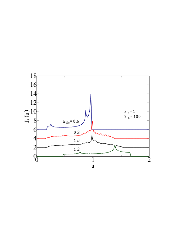
Figure 7: (Color online) System energy distributions $f_{S}(u)$ for $E_{So}=0.5$, 0.8, 1.0 and $1.2$ with $N_{S}=1$, $N_{B}=100$, $T=1.0$ and $c_{o}=1.0$, curves being successively shifted upward by two for clarity of figures.

III.3 Stationary energy probability distributions

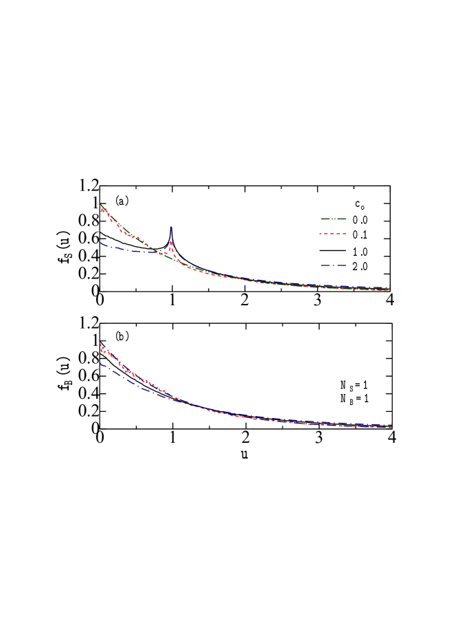
Figure 8: (Color online) Stationary distributions of (a) $f_{S}(u)$ and (b) $f_{B}(u)$ for various $c_{o}$: $c_{o}=0.0$ (double-chain curves), 0.1 (dashed curves), 1.0 (solid curves) and 2.0 (chain curves) obtained by 10 000 runs with $N_{S}=N_{B}=1$ and $T=1.0$.

In this subsection, we will study stationary energy probability distributions of system and bath which are averaged over $N_{r}$ (=10 000) runs stating from different initial conditions. Assuming that the system and bath are in the equilibrium states with $T=u_{B}=u_{S}$ at $t<0.0$, we first generate exponential derivatives of initial system energies $\{E_{j}\}$: $p(E_{j})\propto\exp(-\beta E_{j})$ ($j=1$ to $N_{S}N_{r}$) for our DSs where $\beta=1/k_{B}T$. A pair of initial values of $Q_{j}(0)$ and $P_{j}(0)$ for a given $E_{j}$ is randomly chosen such that they meet the condition given by $E_{j}=P_{j}(0)^{2}/2M+V(Q_{j}(0))$. The procedure for choosing initial values of $q_{n}(0)$ and $p_{n}(0)$ is the same as that adopted in the preceding subsection Hasegawa11 . We have discarded results for $t<200$ in our DSs performed for $t=0$ to 1000.

Before discussing cases where $N_{S}$ and $N_{B}$ may be greater than unity, we first study a pedagogical simple case of $N_{S}=N_{B}=1$: a particle with double-well potential is subjected to a single harmonic oscillator. Double-chain curves in Fig. 8(a) and 8(b) show energy distributions of the system [$f_{S}(u)$] and bath [$f_{B}(u)$], respectively, with $c_{o}=0.0$, where $u=u_{S}$ ($u=u_{B}$) for the system (bath). Both $f_{S}(u_{S})$ and $f_{B}(u_{B})$ follow the exponential distribution because the assumed initial equilibrium states of decoupled system and bath persist at $t\geq 0.0$. When they are coupled by a weak coupling of $c_{o}=0.1$ at $t\geq 0.0$, $f_{S}(u)$ and $f_{B}(u)$ almost remain exponential distributions except for that $f_{S}(u)$ has a small peak at $u=1.0$, as shown by dashed curve in Fig. 8(a). This peak has been realized in Figs. 2(d) and 3(d). It is due to the presence of a potential barrier with $\Delta=1.0$ in double-well potential because the peak at $u=1.0$ in $f_{S}(u)$ is realized even when $T\neq 1.0$, as will be discussed later in 4. Effect of $T$ (Fig. 12). This peak is developed for stronger couplings of $c_{o}=1.0$ and 2.0, for which magnitudes of $f_{S}(u)$ at small $u$ are decreased, as shown by solid and chain curves in Figs. 8(a) and 8(b).

III.3.1 Effect of $c_{o}$

We change the coupling strength of $c_{o}$. Figures 9(a) and 9(b) show $f_{S}(u)$ and $f_{B}(u)$, respectively, for $c_{o}=0.2$, 1.0, 5.0 and 10.0 with $N_{S}=1$, $N_{B}=100$ and $T=1.0$. $f_{S}(u)$ for $c_{o}=0.2$ nearly follows the exponential distribution. When $c_{o}$ becomes larger, magnitudes of $f_{S}(u)$ at $u<1.0$ are decreased while that at $u>1.0$ is increased. In particular, the magnitude of $f_{S}(0)$ is more decreased for larger $c_{o}$.

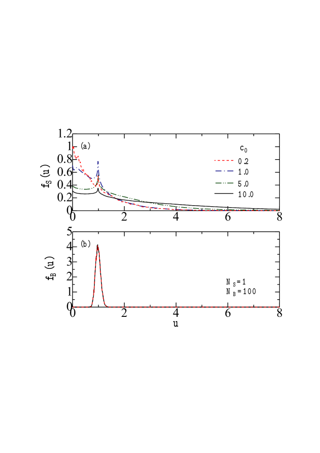
Figure 9: (Color online) Stationary distributions of (a) $f_{S}(u)$ and (b) $f_{B}(u)$ for various $c_{o}$: $c_{o}=0.2$ (dashed curves), 1.0 (chain curves), 5.0 (double-chain curves) and 10.0 (solid curves) with $N_{S}=1$, $N_{B}=100$ and $T=1.0$.

III.3.2 Effect of $\omega_{n}$ distributions

Although we have assumed $\omega_{n}=1.0$ in bath oscillators, we will examine the effect of their distribution, taking into account two kinds of random distributions given by $\omega_{n}\in[0.5,2.0]$ and $\omega_{n}\in[2.0,3.0]$. From calculated results shown in Figs. 10(a) and 10(b), we note that $f_{S}(u)$ and $f_{B}(u)$ are not much sensitive to the distribution of $\{\omega_{n}\}$ in accordance with our previous calculation for harmonic oscillator system Hasegawa11 ; Note1 . This conclusion, however, might not be applied to the case of infinite bath where distribution of $\{\omega_{n}\}$ becomes continuous distribution. Ref. Wei09 reported that the relative position between oscillating frequency ranges of system and bath is very important for a thermalization of the harmonic oscillator system subjected to finite bath.

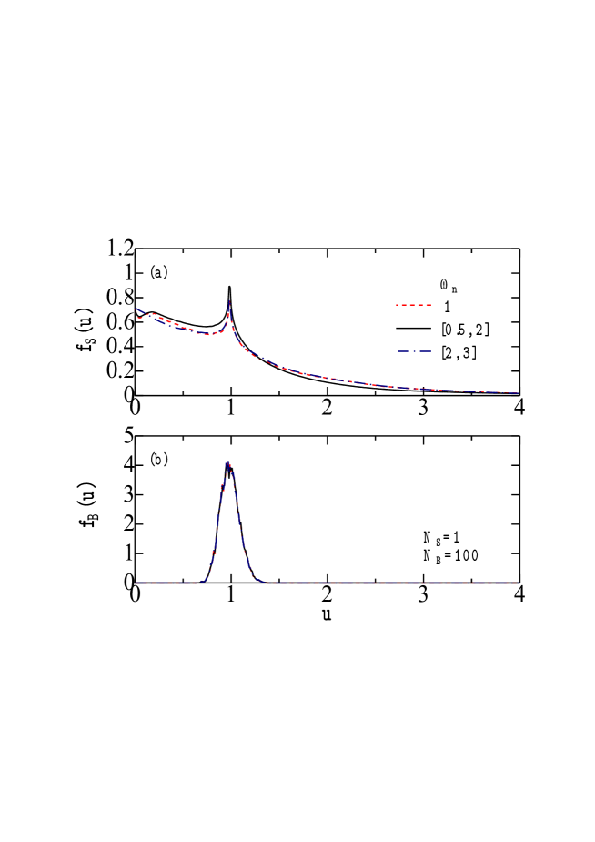
Figure 10: (Color online) Stationary distributions of (a) $f_{S}(u)$ and (b) $f_{B}(u)$ for various distributions of $\{\omega_{n}\}$: $\omega=1.0$ (dashed curves), $\omega_{n}\in[0.5,2.0]$ (solid curves) and $\omega_{n}\in[2.0,3.0]$ (chain curves) with $N_{S}=1$, $N_{B}=100$, $T=1.0$ and $c_{o}=1.0$.

III.3.3 Effect of $N_{B}$

We have calculated $f_{S}(u)$ and $f_{B}(u)$, changing $N_{B}$ but with fixed $N_{S}=1$, whose results are shown in Figs. 11(a) and 11(b). For larger $N_{B}$, the width of $f_{B}(u)$ becomes narrower as expected. However, shapes of $f_{S}(u)$ are nearly unchanged for all cases of $N_{B}=1$, 10, 100 and 1000.

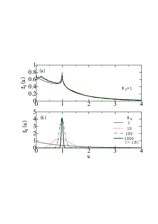
Figure 11: (Color online) Stationary distributions of (a) $f_{S}(u)$ and (b) $f_{B}(u)$ for various $N_{B}$: $N_{B}=1$ (solid curves), 10 (dashed curves), 100 (chain curves) and 1000 (bold solid curves) with $N_{S}=1$, $T=1.0$ and $c_{o}=1.0$. $f_{B}(u)$ for $N_{B}=1000$ is multiplied by a factor of $1/3$.

III.3.4 Effect of $T$

We change the temperature of the bath. Figures 12(a) and 12(b) show $f_{S}(u)$ and $f_{B}(u)$, respectively, for $T=0.5$, 1.0 and 1.5 with $N_{S}=1$, $N_{B}=100$ and $c_{o}=1.0$. When $T$ is decreased (increased), positions of $f_{B}(u)$ move to lower (higher) energy such that mean values of $u_{B}$ correspond to $T$. For a lower temperature of $T=0.5$, magnitude of $f_{S}(u)$ at $u<1.0$ is increased while that at $u>1.0$ is decreased. The reverse is realized for higher temperature of $T=1.5$. We should note that the peak position in $f_{S}(u)$ at $u=1.0$ is not changed even if $T$ is changed because this peak is related to the barrier with $\Delta=1.0$ of the double-well potential.

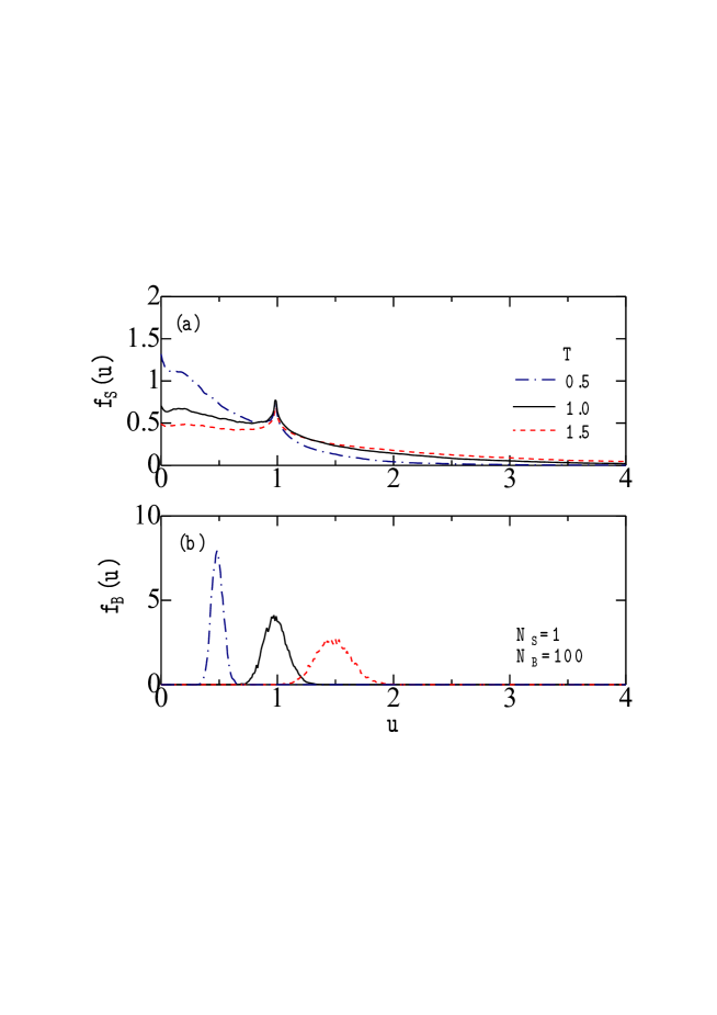
Figure 12: (Color online) Stationary distributions of (a) $f_{S}(u)$ and (b) $f_{B}(u)$ for various $T$: $T=0.5$ (chain curves), 1.0 (solid curves) and 1.5 (dashed curves) with $N_{S}=1$, $N_{B}=100$ and $c_{o}=1.0$.

III.3.5 Effect of $N_{S}$

Although $N_{S}=1$ has been adopted so far, we will change $N_{s}$ to investigate its effects on stationary energy distributions. Figure 13(a) shows $f_{S}(u)$ for $N_{S}=1$, 2, 5 and 10. $f_{S}(u)$ for $N_{S}=1$ shows an exponential-like distribution with $f_{S}(0)\neq 0$ at $u=0.0$. In contrast, $f_{S}(u)$ vanishes at $u=0.0$ for $N_{S}=2$, 5 and 10. Figure 13(a) shows that shapes of $f_{S}(u)$ much depend on $N_{S}$ while those of $f_{B}(u)$ are almost unchanged in Fig. 13(b).

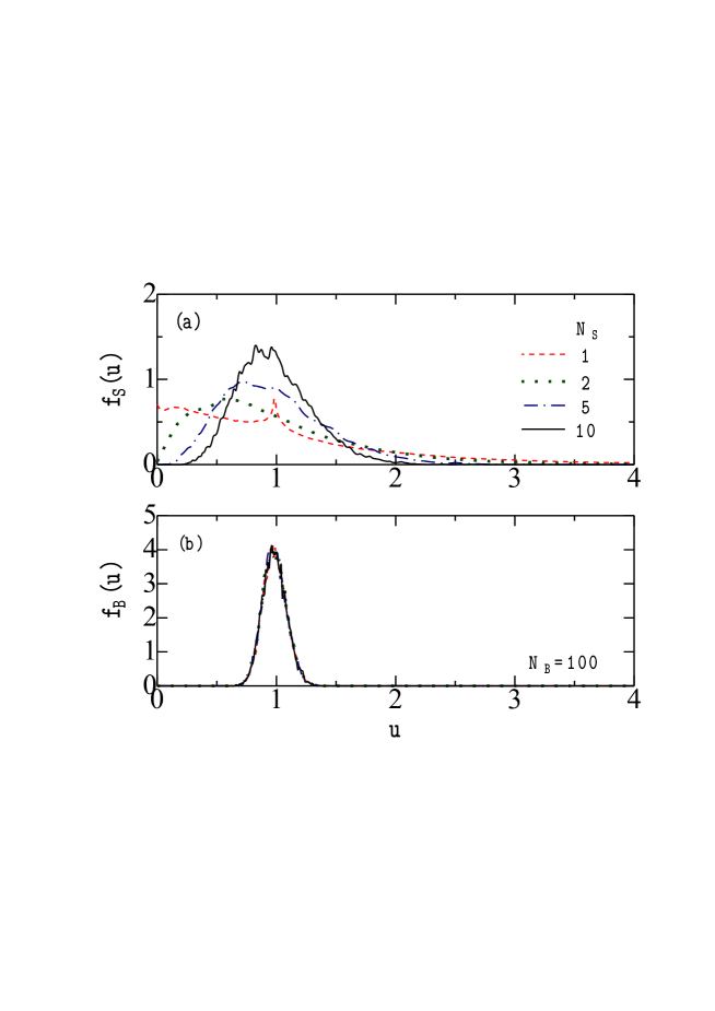
Figure 13: (Color online) Stationary distributions of (a) $f_{S}(u)$ and (b) $f_{B}(u)$ for various $N_{S}$: $N_{S}=1$ (dashed curves), 2 (doted curves), 5 (chain curves) and 10 (solid curves) with $N_{B}=100$, $T=1.0$ and $c_{o}=1.0$.

IV Discussion

IV.1 Analysis of stationary energy distributions

Our DSs in the preceding section have shown that $f_{S}(u)$ depends mainly on $N_{S}$, $c_{o}$ and $T$ while $f_{B}(u)$ depends mostly on $N_{B}$ and $T$ for $N_{S}\ll N_{B}$. We will try to analyze $f_{S}(u)$ and $f_{B}(u)$ in this subsection. It is well known that when variables of $x_{i}$ ($i=1-N$) are independent and follow the exponential distributions with the same mean, the distribution of its sum: $X=\sum_{i}x_{i}$ is given by the $\Gamma$ distribution. Then for an uncoupled system ($c_{o}=0.0$), $f_{S}(u)$ and $f_{B}(u)$ are expressed by the $\Gamma$ distribution $g(u)$ given by Hasegawa11

$$f_{\eta}(u) = \frac{1}{Z_{\eta}}\;u^{a_{\eta}-1}\>e^{-b_{\eta}\>u}\equiv g(u;a_{\eta},b_{\eta}),$$ (28)

with

$$a_{\eta} = N_{\eta},\hskip 28.45274ptb_{\eta}=N_{\eta}\beta,$$ (29)

$$Z_{\eta} = \frac{\Gamma(a_{\eta})}{b_{\eta}^{a_{\eta}}},$$ (30)

where $\eta=$S and B for a system and bath, respectively, and $\Gamma(x)$ is the gamma function. In the limit of $N_{S}=1$, the $\Gamma$ distribution reduces to the exponential distribution. Mean ($\mu_{\eta}$) and variance ($\sigma_{\eta}^{2}$) of the $\Gamma$ distribution are given by

$$\mu_{\eta} = \frac{a_{\eta}}{b_{\eta}},\hskip 28.45274pt\sigma_{\eta}^{2}=\frac{a_{\eta}}{b_{\eta}^{2}},$$ (31)

from which $a_{\eta}$ and $b_{\eta}$ are expressed in terms of $\mu_{\eta}$ and $\sigma_{\eta}$

$$a_{\eta} = \frac{\mu_{\eta}^{2}}{\sigma_{\eta}^{2}},\hskip 28.45274ptb_{\eta}=\frac{\mu_{\eta}}{\sigma_{\eta}^{2}}.$$ (32)

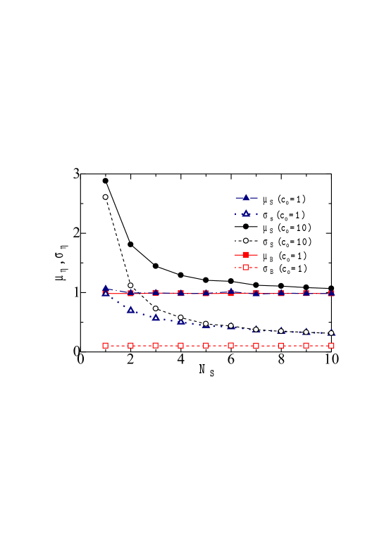
Figure 14: (Color online) $N_{S}$ dependences of $\mu_{\eta}$ and $\sigma_{\eta}$ of system ($\eta=S$) and bath $(\eta=B)$ with $N_{B}=100$ and $T=1.0$: filled (open) triangles denote $\mu_{S}$ ($\sigma_{S}$) with $c_{o}=1.0$: filled (open) circles express $\mu_{S}$ ($\sigma_{S}$) with $c_{o}=10.0$: filled (open) squares show $\mu_{B}$ ($\sigma_{B}$) with $c_{o}=1.0$.

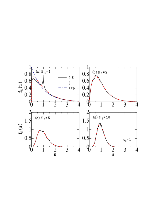
Figure 15: (Color online) $u$ dependences of $f_{S}(u)$ for (a) $N_{S}=1$, (b) $N_{S}=2$, (c) $N_{S}=5$ and (d) $N_{S}=10$ with $T=1.0$, $c_{o}=1.0$ and $N_{B}=100$ obtained by DSs (solid curves): dashed and chain curves express $\Gamma$ and exponential distributions, respectively (see text).

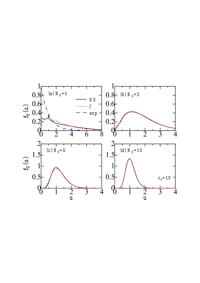
Figure 16: (Color online) $u$ dependences of $f_{S}(u)$ for (a) $N_{S}=1$, (b) $N_{S}=2$, (c) $N_{S}=5$ and (d) $N_{S}=10$ with $T=1.0$, $c_{o}=10.0$ and $N_{B}=100$ obtained by DSs (solid curves): dashed and chain curves express $\Gamma$ and exponential distributions, respectively (see text).

We have tried to evaluate $f_{S}(u)$ and $f_{B}(u)$ for the coupled system ($c_{o}\neq 0.0$) as follows: From mean ($\mu_{\eta}$) and root-mean-square (RMS) ($\sigma_{\eta}$) calculated by DSs, $a_{\eta}$ and $b_{\eta}$ are determined by Eq. (32), with which we obtain the $\Gamma$ distributions for $f_{S}(u)$ and $f_{B}(u)$. Filled and open squares in Fig. 14 show $\mu_{B}$ and $\sigma_{B}$, respectively, as a function of $N_{S}$. We obain $\mu_{B}=1.0$ and $\sigma_{B}=0.1$ nearly independently of $N_{S}$, which yield $a_{B}=b_{B}=100.0$ in agreement with Eq. (29). Filled and open triangles in Fig. 14 express the $N_{S}$ dependence of $\mu_{S}$ and $\sigma_{S}$ obtained by DSs with $c_{o}=1.0$, $N_{B}=100$ and $T=1.0$. Calculated mean and RMS values of $(\mu_{S},\sigma_{S})$ are $(1.07,0.98)$, $(0.99,0.70)$, $(0.99,0.44)$ and $(0.99,0.319)$ for $N_{S}=1$, 2, 5 and 10, respectively, for which Eq. (32) yields $(a_{S},b_{S})=(1.18,1.11)$, $(2.04,2.05)$, $(4.50,5.06)$ and $(9.82,9.97)$. These values of $a_{S}$ and $b_{S}$ are not so different from $N_{S}$ and $N_{S}\beta$ given by Eq. (29). We have employed the $\Gamma$ distribution with these parameters $a_{S}$ and $b_{S}$ for our analysis of $f_{S}(u)$ having been shown in Fig. 13(a). Dashed curves in Figs. 15(a)-(d) express calculated $\Gamma$ distributions, which are in fairly good agreement with $f_{S}(u)$ plotted by solid curves, except for $N_{S}=1$ for which $g(0)=0.0$ because $a_{S}=1.18>1.0$ while $f_{S}(0)\neq 0.0$.

Similar analysis has been made for another result obtained with a larger $c_{o}=10.0$ for $N_{B}=100$ and $T=1.0$. $N_{S}$-dependences of calculated $\mu_{S}$ and $\sigma_{S}$ are plotted by filled and open circles, respectively, in Fig. 14. Calculated $(\mu_{S},\sigma_{S})$ are $(2.88,2.61)$, $(1.81,1.12)$, $(1.21,0.47)$ and $(1.07,0.31)$ for $N_{S}=1$, 2, 5 and 10, respectively, which lead to $(a_{S},b_{S})=(1.22,0.42)$, $(2.62,1.45)$, $(6.57,5.44)$ and $(11.54,10.81)$ by Eq. (32). Obtained $a_{S}$ and $b_{S}$ are rather different from $N_{S}$ and $N_{S}\beta$ given by Eq. (29). Dashed curves in Figs. 16(a)-(d) show $\Gamma$ distributions with these parameters, which may approximately explain $f_{S}(u)$ obtained by DSs in the phenomenologically sense, except for $N_{S}=1$ for which $g(0)=0.0$ but $f_{S}(0)\neq 0.0$.

We note in Fig. 15(a) or 16(a) that an agreement between $g(u)$ and $f_{S}(u)$ with $N_{S}=1$ is not satisfactory. We have tried to obtain a better fit between them, by using the $q$-$\Gamma$ distribution $g_{q}(u)$ given by Hasegawa11

$$g_{q}(u) = \frac{1}{Z_{q}}\>u^{a-1}\>e_{q}^{-bu},$$ (33)

with

$$e_{q}^{x} = [1+(1-q)x]_{+}^{1/(1-q)},$$ (34)

where $[y]_{+}=\max(y,0)$ and $Z_{q}$ is the normalization factor. Note that $g_{q}(u)$ reduces to the $\Gamma$ distribution in the limit of $q\rightarrow 1.0$. Although the $q$-$\Gamma$ distribution was useful for $f_{S}(u)$ of harmonic-oscillator systems subjected to finite bath Hasegawa11 , it does not work for $f_{S}(u)$ of double-well systems. This difference may be understood from a comparison between $f_{S}(u)$ for $N_{S}=1$ of a double-well system shown in Fig. 15(a) [or 16(a)] and its counterpart of a harmonic oscillator system shown in Fig. 9(a) of Ref. Hasegawa11 . Although the latter shows an exponential-like behavior with a monotonous decrease with increasing $u$, the former with a characteristic peak at $u=1.0$ cannot be expressed by either the exponential, $\Gamma$, or $q$-$\Gamma$ distribution.

IV.2 Analysis of stationary position distributions

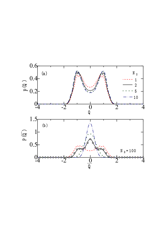
Figure 17: (Color online) Stationary distributions of (a) $p(Q)$ as a function of particle position $Q$ and (b) $P(\bar{Q})$ as a function of the averaged position $\bar{Q}$ for various $N_{S}$: $N_{S}=1$ (dashed curve), 2 (solid curve), 5 (dotted curve) and 10 (chain curve) with $N_{B}=100$, $T=1.0$ and $c_{o}=1.0$. Open circles in (b) express an analytical result obtained by Eq. (36) with $N_{S}=2$.

We have studied also the $N_{S}$ dependence of stationary position distributions of $p(Q)$ and $P(\bar{Q})$, where $Q$ denotes the position of a particle in the system and $\bar{Q}$ expresses the averaged position given by

$$\bar{Q} = \frac{1}{N_{S}}\sum_{k=1}^{N_{S}}Q_{k}.$$ (35)

Figures 17(a) and 17(b) show $p(Q)$ and $P(\bar{Q})$, respectively, obtained by DSs for various $N_{S}$ with $N_{B}=100$, $T=1.0$ and $c_{o}=1.0$. For $N_{S}=1$, we obtain $p(Q)=P(\bar{Q})$ with the characteristic double-peaked structure. We note, however, that $P(\bar{Q})$ is different from $p(Q)$ for $N_{S}>1$ for which $P(\bar{Q})$ has a single-peaked structure despite the double-peaked $p(Q)$. This is easily understood as follows: For example, in the case of $N_{S}=2$, two particles in the system mainly locate at $Q_{k}=1.0$ or $Q_{k}=-1.0$ ($k=1,2$) which yields the double-peaked distribution of $f_{S}(Q)$. However, the averaged position of $\bar{Q}=(Q_{1}+Q_{2})/2$ will be dominantly $\bar{Q}=0.0$, which leads to a single-peaked $P(\bar{Q})$. The situation is the same also for $N_{S}>2$.

Theoretically $P(\bar{Q})$ may be expressed by

$$P(\bar{Q}) = \int\cdot\cdot\int\prod_{k=1}^{N_{S}}\>dQ_{k}\;\exp\left[-\beta V(Q_{k})\right]\>\delta\left(\bar{Q}-N_{S}^{-1}\sum_{k=1}^{N_{S}}Q_{k}\right).$$ (36)

$P(\bar{Q})$ numerically evaluated for $N_{S}=2$ is plotted by open circles in Fig. 17 which are in good agreement with the solid curve expressing $P(\bar{Q})$ obtained by DS. It is impossibly difficult to numerically evaluate Eq. (36) for $N_{S}\geq 3$. In the limit of $N_{S}\rightarrow\infty$, $P(\bar{Q})$ reduces to the Gaussian distribution according to the central-limit theorem. This trend is realized already in the case of $N_{S}=10$ in Fig. 17(b).

V Concluding remarks

We have studied the properties of classical double-well systems coupled to finite bath, employing the ($N_{S}+N_{B}$) model Hasegawa11 in which $N_{S}$-body system is coupled to $N_{B}$-body bath. Results obtained by DSs have shown the following:

(i) Chaotic oscillations are induced in the double-well system coupled to finite bath in the absence of external forces for appropriate model parameters of $c_{o}$, $N_{B}$, $T$, $\{\omega_{n}\}$ and $E_{So}$,

(ii) Among model parameters, $f_{S}(u)$ depends mainly on $N_{S}$, $c_{o}$ and $T$ while $f_{B}(u)$ depends on $N_{B}$ and $T$ for $N_{S}\ll N_{B}$,

(iii) $f_{S}(u)$ for $N_{S}>1$ obtained by DSs may be phenomenological expressed by the $\Gamma$ distribution,

(iv) $f_{S}(u)$ for $N_{S}=1$ with $c_{o}\neq 0.0$ cannot be described by either the exponential, $\Gamma$, or $q$-$\Gamma$ distribution, although that with $c_{o}=0.0$ follows the exponential distribution, and

(v) The dissipation is not realized in the system energy for DSs at $t=0-1000$ with $N_{S}=1-100$ and $N_{B}=10-1000$.

The item (i) is in consistent with chaos in a closed classical double-well system driven by external forces Reichl84 , although chaos is induced without external forces in our open classical double-well system. This is somewhat reminiscent of chaos induced by quantum noise in the absence of external force in closed quantum double-well systems Pattanayak94 . Effects of induced chaos in the item (i) are not apparent in $f_{S}(u)$ because $u$ ($=u_{S}$) is ensemble averaged over 10 000 runs (realizations) with exponentially distributed initial system energies. Items (ii) and (v) are the same as in the harmonic-oscillator system coupled to finite bath Hasegawa11 . The item (v) suggests that for the energy dissipation of system, we might need to adopt a much larger $N_{B}$ ($\gg 1000$) Poincare . The item (iv) is in contrast to $f_{S}(u)$ for $N_{S}=1$ in the open harmonic-oscillator system which may be approximately accounted for by the $q$-$\Gamma$ distribution Hasegawa11 . It would be necessary and interesting to make a quantum extension of our study which is left as our future subject.

- (1) A. O. Caldeira and A. J. Leggett, Phys. Rev. Lett. 46, 211 (1981).
- (2) A. O. Caldeira and A. J. Leggett, Ann. Phys. 149, 374 (1983).
- (3) V. B. Magalinskii, Sov. Phys. JETP 9, 1381 (1959).
- (4) P. Ullersma, Physica 32, 27 (1966); ibid. 32, 56 (1966); ibid. 32, 74 (1966); ibid. 32, 90 (1966).
- (5) P. Hanggi, Gert-Ludwig Ingold and P. Talkner, New Journal of Physics 10, 115008 (2008).
- (6) Gert-Ludwig Ingold, P. Hanggi, and P. Talkner, Phys. Rev. E 79, 061105 (2009).
- (7) S. T. Smith and R. Onofrio, Eur. Phys. J. B 61 , 271 (2008).
- (8) Q. Wei, S. T. Smith, and R. Onofrio, Phys. Rev. E 79, 031128 (2009).
- (9) J. Rosa and M. W. Beims, Phys. Rev. E 78, 031126 (2008).
- (10) H. Hasegawa, Phys. Rev. E 83, 021104 (2011).
- (11) A. Carcaterra, and A. Akay, Phys. Rev. E 84, 011121 (2011).
- (12) H. Hasegawa, J. Math. Phys. 52, 123301 (2011).
- (13) H. Hasegawa, Phys, Rev. E 84, 011145 (2011).
- (14) C. Jarzynski, Phys. Rev. Lett. 78, 2690 (1997); Phys. Rev. E 56, 5018 (1997).
- (15) M. Thorwart, M. Grifoni, and P. Hänggi, Annals Phys. 293, 14 (2001).
- (16) H. Hasegawa, arXiv:1205.2058.
- (17) L. Gammaitoni, P. Hänggi, P. Jung, and F. Marchesoni, Rev. Mod. Phys. 70, 223 (1998).
- (18) P. Hänggi, F. Marchesoni, and P. Grigolini, Z. Phys. B 56, 333 (1984).
- (19) P. Hänggi, , P. Jung, C. Zerbe, and F. Moss, 1993, J. Stat. Phys. 70, 25 (1993).
- (20) L. Gammaitoni, E. Menichella-Saetta, S. Santucci, F. Marchesoni, and C. Presilla, Phys. Rev. A 40, 2144 (1989).
- (21) A. Neiman and W. Sung, Phys. Lett. A 223, 341 (1996).
- (22) H. Hasegawa, arXiv:1203.0770.
- (23) L. E. Reichl and W. M. Zheng, Phys. Rev. A 29, 2186 (1984).
- (24) In the CL model ( and ), we assume (: constant) because the kernel includes the term as given by which becomes in the limit of , denoting the spectral density [see Eq. (20)].
- (25) A careless mistake was realized in of Fig. 6(c) in Ref. Hasegawa11 , which should be nearly the same as that of Fig. 10(b) in this paper.
- (26) The recurrence time in a finite system is finite in the Poincaré recurrence theorem: H. Poincaré, Acta Math. 13, 1 (1890), see also S. Chandrasekhar, Rev. Mod. Phys. 15, 1 (1943).
- (27) A. K. Pattanayak and W. C. Schieve, Phys. Rev. Lett. 72, 2855 (1994).