Continuous-variable blind quantum computation

Abstract

Blind quantum computation is a secure delegated quantum computing protocol where Alice who does not have sufficient quantum technology at her disposal delegates her computation to Bob who has a fully-fledged quantum computer in such a way that Bob cannot learn anything about Alice’s input, output, and algorithm. Protocols of blind quantum computation have been proposed for several qubit measurement-based computation models, such as the graph state model, the Affleck-Kennedy-Lieb-Tasaki model, and the Raussendorf-Harrington-Goyal topological model. Here, we consider blind quantum computation for the continuous-variable measurement-based model. We show that blind quantum computation is possible for the infinite squeezing case. We also show that the finite squeezing causes no additional problem in the blind setup apart from the one inherent to the continuous-variable measurement-based quantum computation.

I Introduction

When scalable quantum computers are realized, they will be used in “cloud computing style” since only limited number of people will be able to possess quantum computers. Blind quantum computation Childs ; Arrighi ; blindcluster ; Aha ; TVE ; Vedran ; Barz ; blind_Raussendorf ; FK ; measuringAlice provides a solution to the issue of the client’s security in such a cloud quantum computation. Blind quantum computation is a new secure protocol which enables Alice who does not have enough quantum technology to delegate her computation to Bob who has a fully-fledged quantum computer in such a way that Bob cannot learn anything about Alice’s input, output, and algorithm. A protocol of the unconditionally secure universal blind quantum computation for almost classical Alice was first proposed in Ref. blindcluster by using the measurement-based quantum computation (MBQC) on the cluster state cluster ; cluster2 ; Raussendorf_PhD , and later generalized to other resource states such as the Affleck-Kennedy-Lieb-Tasaki state TVE ; MiyakeAKLT ; AKLT and the three-dimensional Raussendorf-Harrington-Goyal state Raussendorf_PRL ; Raussendorf_NJP ; Raussendorf_Ann ; Li_finiteT ; FM_finiteT which enables the topological protection blind_Raussendorf ; FK . A subroutine which eases Alice’s burden was invented Vedran . Also, a verification scheme which tests Bob’s honesty was proposed FK . The proof-of-principle experiment of the original protocol blindcluster was realized in an optical system Barz .

In this paper, we consider the continuous-variable (CV) version of the blind quantum computation. The CV cluster MBQC was proposed in Refs. canonical_full ; canonical_letter ; review . There,

$$|+\rangle\equiv\frac{1}{\sqrt{2}}(|0\rangle+|1\rangle)$$

state of a single qubit is replaced with the zero momentum state $|0\rangle_{p}$ of a single mode (qumode), and the two-mode gate $e^{iq\otimes q}$ plays the role of the qubit Controlled-Z gate,

$$|0\rangle\langle 0|\otimes I+|1\rangle\langle 1|\otimes Z.$$

Experimental demonstrations of building blocks of the CV cluster MBQC were already achieved experiment1 ; experiment2 ; experiment3 ; experiment5 ; experiment6 .

We show that blind quantum computation is possible in the infinite squeezing case. We also consider the finite squeezing case, and show that the finite squeezing causes no problem apart from the additional errors which come from the redundancy of gates required for the blindness. Since these errors are those even the non-blind CV MBQC has to cope with for its scalability, we conclude that the finite squeezing does not cause any fundamental problem in principle.

This paper is organized as follows. In the next section we will briefly review the CV cluster MBQC. We also review the qubit blind quantum computation in Sec. III. Then we explain our protocol in Sec. IV, and show its correctness (Sec. V) and blindness (Sec. VI). Discussions are given in Sec. VII.

II CV cluster MBQC

Let us briefly review the CV cluster MBQC proposed in Refs. canonical_letter ; canonical_full . Let $q$ and $p$ be the quadrature “position” and “momentum” operators, respectively, satisfying the canonical commutation relation

$$[q,p]=i.$$

We also define the Weyl-Heisenberg operators

$$X(s) \equiv \exp[-isp],$$

$$Z(s) \equiv \exp[isq],$$

with $s\in{\mathbb{R}}$, where

$$X(s)|t\rangle_{q} = |t+s\rangle_{q},$$

$$Z(s)|t\rangle_{p} = |t+s\rangle_{p}.$$

Here, $|t\rangle_{q}$ and $|t\rangle_{p}$ are eigenvectors of $q$ and $p$ with the eigenvalue $t$, respectively. They satisfy

$$X(s)Z(t)=e^{-ist}Z(t)X(s),$$

$$qX(s)=X(s)(q+s),$$

$$pZ(s)=Z(s)(p+s).$$

These Weyl-Heisenberg operators are CV analog of the qubit Pauli operators. The Fourier transform operator $F$ is defined by

$$F\equiv\exp\Big{[}i(q^{2}+p^{2})\frac{\pi}{4}\Big{]},$$

with

$$F|s\rangle_{q}=|s\rangle_{p}.$$

This operator is the CV analog of the qubit Hadamard operator. However, special cares are needed because $F$ is not Hermitian and

$$F^{2}|s\rangle_{q} = |-s\rangle_{q},$$

$$F^{2}|s\rangle_{p} = |-s\rangle_{p},$$

$$F^{4} = I,$$

$$F^{\dagger}qF = -p,$$

$$F^{\dagger}pF = q,$$

$$Z(m)F = FX(m),$$

$$X(m)F = FZ(-m).$$

The CV version of the Controlled-$Z$ gate are defined by

$$CZ\equiv\exp(iq\otimes q).$$

Note that we use the symbol $CZ$ for both qubit $CZ$ and CV $CZ$. But no confusion will occur because they can be distinguished from the context. The CV version of the Controlled-$X$ gate is defined by

$$CX\equiv\exp(-iq\otimes p).$$

The elementary block of the CV cluster MBQC is the teleportation gate given in Fig. 1. Here,

$$D_{q}^{f}\equiv\exp[if(q)],$$

and $f$ is a polynomial of $q$. Note that $D_{q}^{f}$ and $D_{p}^{f}$ are obtained from $FD_{q}^{f}$, since

$$(FD_{q}^{0})^{3}FD_{q}^{f} = D_{q}^{f},$$

$$(FD_{q}^{0})^{2}(FD_{-q}^{f})(FD_{q}^{0}) = D_{p}^{f}.$$

Furthermore, $e^{isq^{k}/k}$ $(k=1,2,3)$ and $e^{isp^{k}/k}$ $(k=1,2,3)$ are single-mode universal Lloyd . Hence

$$R_{q}(v)\equiv F\exp\Big{[}i\Big{(}aq+b\frac{q^{2}}{2}+c\frac{q^{3}}{3}\Big{)}\Big{]}$$

is single-mode universal, where $v=(a,b,c)$. Addition of $CZ$ enables all multi-mode universality.

Let us explain how to compensate the byproduct error $X(m)$. Note that

$$R_{q}(v)X(m) = Z(m)R_{q+m}(v),$$

$$= Z(m)R_{q}(M_{m}v),$$

where

$$M_{m}=\left(\begin{array}[]{ccc}1&m&m^{2}\\ 0&1&2m\\ 0&0&1\end{array}\right)$$

and its inverse is

$$M_{m}^{-1}=\left(\begin{array}[]{ccc}1&-m&m^{2}\\ 0&1&-2m\\ 0&0&1\end{array}\right).$$

Therefore, if we want to implement $R_{q}(v)$, and if there is the byproduct $X(m)$, we have only to implement $R_{q}(M_{m}^{-1}v)$. Furthermore, we can show

$$CZ(X(m)\otimes I) = (X(m)\otimes Z(m))CZ,$$

$$CZ(I\otimes X(m)) = (Z(m)\otimes X(m))CZ.$$

Therefore, the byproducts can be sent forward through $CZ$ gates. In short, Fig. 2 (a) is universal if the feed-forwarding is appropriately done.

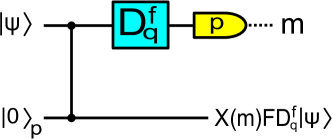
Figure 1: (Color online.) The CV teleportation gate.

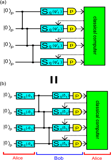
Figure 2: (Color online.) (a): $S_{q}(\phi)$ stands for $F^{\dagger}R_{q}(\phi)$. This circuit is universal if $\{\phi^{\prime}_{j}\}$ are appropriately chosen according to the previous measurement results. (b): The blind version of (a). Obviously, $S_{q}$’s commute with $CZ$’s, and therefore (b) is equivalent to (a).

The application of $D_{q}^{f}$ followed by the measurement of $p$ is equivalent to the measurement of the observable $(D_{q}^{f})^{\dagger}pD_{q}^{f}$. Therefore, to implement the gate $e^{isq}$ in Fig. 1, we measure

$$e^{-isq}pe^{isq}=p+s.$$

It can be measured easily with a homodyne detection. To implement the gate $e^{isq^{2}/2}$ in Fig. 1, we measure

$$e^{-isq^{2}/2}pe^{isq^{2}/2}=p+sq.$$

It can also be measured with a homodyne detection in a rotated quadrature basis. In principle, the gate $e^{isq^{3}/3}$ can be implemented in Fig. 1 by measuring

$$e^{-isq^{3}/3}pe^{isq^{3}/3}=p+sq^{2}.$$

Finally, let us notice that the zero-momentum state $|0\rangle_{p}$ is not realistic, and normally $|0\rangle_{p}$ is approximated by the finitely squeezed vacuum state

$$|0,\Omega\rangle_{p}=\frac{1}{(\pi\Omega^{2})^{1/4}}\int dp~{}e^{-\frac{p^{2}}{2\Omega^{2}}}|p\rangle_{p}.$$

This finite squeezing causes errors in the CV cluster MBQC canonical_letter ; canonical_full .

III Blind quantum computation

Let us also briefly review the basic idea of the original blind quantum computation protocol of Ref. blindcluster . For details, see Refs. blindcluster ; TVE ; Vedran ; Barz ; blind_Raussendorf ; FK ; measuringAlice . Alice, the client, has a quantum device which emits randomly-rotated single qubit states and a classical computer. Bob, the server, has a full quantum power. Let us assume that Alice wants to perform the cluster MBQC on the $N$-qubit graph state $|G\rangle$ with measurement angles $\{\phi_{j}\}_{j=1}^{N}$. If Alice sends Bob $\{\phi_{j}\}_{j=1}^{N}$, and Bob creates $|G\rangle$, the delegated quantum computation is of course possible. However, obviously, in this case Bob can learn Alice’s privacy. Hence they run the following protocol:

1. Alice sends Bob $N$ randomly-rotated single-qubit states $\{|+_{\theta_{j}}\rangle\}_{j=1}^{N}$, where

   $$|+_{\theta}\rangle\equiv\frac{1}{\sqrt{2}}(|0\rangle+e^{i\theta}|1\rangle)=e^{-iZ\theta/2}|+\rangle$$

   and

   $$\theta_{j}\in\Big{\{}\frac{k\pi}{4}~{}\Big{|}k=0,1,...,7\Big{\}}$$

   is a random angle which is hidden to Bob.

2. Bob applies $CZ$ gates among them. Since $CZ$ commutes with $e^{-iZ\theta/2}$, what Bob obtains is

   $$\Big{(}\bigotimes_{e\in E}CZ_{e}\Big{)}\Big{(}\bigotimes_{j=1}^{N}e^{-iZ_{j}\theta_{j}/2}\Big{)}|+\rangle^{\otimes N}$$

   $$= \Big{(}\bigotimes_{j=1}^{N}e^{-iZ_{j}\theta_{j}/2}\Big{)}\Big{(}\bigotimes_{e\in E}CZ_{e}\Big{)}|+\rangle^{\otimes N}$$

   $$= \Big{(}\bigotimes_{j=1}^{N}e^{-iZ_{j}\theta_{j}/2}\Big{)}|G\rangle,$$

   where $E$ is the set of edges of $G$, and the subscript $j$ of $Z_{j}$ means the operator acts on $j$th qubit.

3. For $j=1$ to $N$ in turn:

   1. Alice sends Bob

      $$\delta_{j}\equiv\theta_{j}+\phi_{j}^{\prime}+r_{j}\pi,$$

      where $\phi_{j}^{\prime}$ is the modification of $\phi_{j}$ which includes appropriate feedforwardings (byproduct corrections) and $r_{j}\in\{0,1\}$ is a random binary.

   2. Bob does the measurement in the $\{|\pm_{\delta_{j}}\rangle\}$ basis, and returns the measurement result to Alice.

It was shown in Ref. blindcluster that this protocol is correct. Here, correct means that if Bob is honest Alice obtains the correct outcome. In fact, if Bob measures $k$th qubit in the $\{|\pm_{\delta_{k}}\rangle\}$ basis,

$$\langle\pm_{\delta_{k}}|\Big{(}\bigotimes_{j=1}^{N}e^{-iZ_{j}\theta_{j}/2}\Big{)}|G\rangle$$

$$= \langle\pm|e^{iZ_{k}\delta_{k}/2}\Big{(}\bigotimes_{j=1}^{N}e^{-iZ_{j}\theta_{j}/2}\Big{)}|G\rangle$$

$$= \Big{(}\bigotimes_{j\neq k}e^{-iZ_{j}\theta_{j}/2}\Big{)}\langle\pm|e^{iZ_{k}\delta_{k}/2}e^{-iZ_{k}\theta_{k}/2}|G\rangle$$

$$= \Big{(}\bigotimes_{j\neq k}e^{-iZ_{j}\theta_{j}/2}\Big{)}\langle\pm|e^{iZ_{k}(\phi_{k}^{\prime}+r_{k}\pi)/2}|G\rangle$$

$$= \Big{(}\bigotimes_{j\neq k}e^{-iZ_{j}\theta_{j}/2}\Big{)}\langle\pm_{\phi_{k}^{\prime}}|Z^{r_{k}}_{k}|G\rangle,$$

which means that Bob effectively does the $\{|\pm_{\phi_{k}^{\prime}}\rangle\}$ basis measurement with the error $Z^{r_{k}}$. The error $Z^{r_{k}}$ just flips the bit of the measurement result, and therefore it can be compensated later.

It was also shown that the protocol is blind blindcluster . Here, blind intuitively means that whatever Bob does, Bob cannot learn anything about Alice’s input, output, and algorithm. Intuitive proof of the blindness is as follows: What Bob obtains are quantum states $\{|+_{\theta_{j}}\rangle\}_{j=1}^{N}$ and classical messages $\{\delta_{j}\}_{j=1}^{N}$. Hence Bob’s state is

$$\sum_{\phi_{1},...,\phi_{N}}\sum_{r_{1},...,r_{N}}\bigotimes_{j=1}^{N}|+_{\phi_{j}^{\prime}+r_{j}\pi}\rangle\langle+_{\phi_{j}^{\prime}+r_{j}\pi}|=I^{\otimes N},$$

which means that Bob cannot learn anything about $\{\phi_{j}\}_{j=1}^{N}$ whichever POVM he does on his system.

In order to guarantee Alice’s privacy, the geometry of the graph $G$ must be secret to Bob. There are three ways of doing it. First one is to use the brickwork state blindcluster . It is a certain two-dimensional graph state which is universal with only $\{|\pm_{\theta}\rangle\}$ basis measurements for $\theta\in\{\frac{k\pi}{4}|k=0,1,...,7\}$. Second one is to implant a “hair” to each qubit of the regular lattice graph state blind_Raussendorf . For example, let us consider the left graph state of Fig. 3. We can simulate $Z$ measurement and any $X-Y$ plane measurement on any blue qubit with only $X-Y$ plane measurements on yellow and blue qubits. Hence we can “carve out” a specific graph state from the square lattice of blue qubits as is shown in the right of Fig. 3. Third one is so called “the graph hiding technique” FK . By using this technique, Alice can have Bob prepare any graph state in such a way that Bob cannot learn the geometry of the graph. This technique is based on the simple idea that $CZ$ does not create entanglement if one of the qubits is $|0\rangle$ or $|1\rangle$:

$$CZ(|\psi\rangle\otimes|+\rangle) = CZ(|\psi\rangle\otimes|+\rangle),$$

$$CZ(|\psi\rangle\otimes|-\rangle) = (I\otimes Z)CZ(|\psi\rangle\otimes|-\rangle),$$

$$CZ(|\psi\rangle\otimes|0\rangle) = |\psi\rangle\otimes|0\rangle,$$

$$CZ(|\psi\rangle\otimes|1\rangle) = Z|\psi\rangle\otimes|1\rangle.$$

Therefore, if Alice hides several qubits in $|0\rangle$ or $|1\rangle$ into the set of qubits she initially sends to Bob, she can let Bob create her desired graph state. Since Bob cannot distinguish $|0\rangle$, $|1\rangle$, and eight $|+_{\theta}\rangle$ states, Bob cannot know when he entangles qubits (Fig. 4).

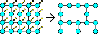
Figure 3: (Color online.) The hair implantation technique blind_Raussendorf . Left: A two-qubit graph state (“hair”) indicated by yellow is attached to each blue qubit of the square graph state. Right: A desired graph state can be carved out from the blue square graph.

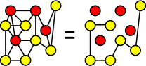
Figure 4: (Color online.) The graph hiding technique FK . Yellow qubits are $|+_{\theta}\rangle$, whereas red qubits are $|0\rangle$ or $|1\rangle$. Bob applies $CZ$ gates on all edges of the left graph, but actually he obtains the right graph state, and he does not know its geometry.

IV CV blind protocol

Now let us consider the CV blind protocol. We here describe the ideal version and later consider realistic situations. Our protocol runs as follows:

1. Alice sends Bob

   $$\Big{\{}S_{q}(-\theta_{j})|0\rangle_{p}\Big{\}}_{j=1}^{N},$$

   where $\theta_{j}=(a_{j},b_{j},c_{j})$ is randomly chosen from ${\mathbb{R}}^{3}$ and $S_{q}(v)=F^{\dagger}R_{q}(v)$.

2. Bob applies $CZ$ gates.

3. Alice and Bob might choose “the brickwork”, “the hair implantation technique”, or “the graph hiding technique”. Irrespective of their choice, we can assume without loss of generality that Bob has the “encrypted” CV graph state

   $$\Big{[}\bigotimes_{j=1}^{N}X^{j}(\xi_{j})Z^{j}(\eta_{j})S_{q}^{j}(-\theta_{j})\Big{]}|G\rangle,$$

   where $|G\rangle$ is the $N$-qumode CV graph state, and the subscript $j$ of $X^{j}$ means it acts on the $j$th qumode.

4. For $j=1$ to $N$ in turn:

   1. Let $\phi_{j}\equiv(\alpha_{j},\beta_{j},\gamma_{j})$ be Alice’s computational parameters, and Let $\phi_{j}^{\prime}\equiv(\alpha^{\prime}_{j},\beta_{j}^{\prime},\gamma_{j}^{\prime})$ be the one including feedforwardings. Alice sends Bob $\delta_{j}=M_{\xi_{j}}^{-1}w_{j}$ where

      $$w_{j}=\left(\begin{array}[]{l}\alpha_{j}^{\prime}+a_{j}-\eta_{j}+r_{j}\\ \beta_{j}^{\prime}+b_{j}\\ \gamma_{j}^{\prime}+c_{j}\end{array}\right)$$

      and $r_{j}\in{\mathbb{R}}$ is a random real number.

   2. Bob applies $S_{q}(\delta_{j})$ on $j$th qumode and does the $p$ measurement on it. (Or he directly measures $S_{q}^{\dagger}(\delta_{j})pS_{q}(\delta_{j})$ of the $j$th qumode.) He sends the measurement result to Alice.

V Correctness

Let us show the correctness of our protocol. See Fig. 2 (b), which is the circuit representation of our protocol. Since $S_{q}$ commutes with $CZ$, Fig. 2 (b) is equivalent to Fig. 2 (a). Note that the equivalence between (a) and (b) in Fig. 2 is based on only the commutativity between $S_{q}$ and $CZ$, and therefore it holds even if we replace each input $|0\rangle_{p}$ with its finitely squeezed version. Hence, the finite squeezing does not cause any additional effect here.

More precisely, note that the following is true for any state $|\psi\rangle$:

$${}_{p}\langle p|S_{q}^{j}(\delta_{j})X^{j}(\xi_{j})Z^{j}(\eta_{j})S_{q}^{j}(-\theta_{j})|\psi\rangle$$

$$= {}_{p}\langle p|X^{j}(\xi_{j})Z^{j}(\eta_{j})S_{q}^{j}(M_{\xi_{j}}M_{\xi_{j}}^{-1}w_{j})S_{q}^{j}(-\theta_{j})|\psi\rangle$$

$$= {}_{p}\langle p|X^{j}(\xi_{j})Z^{j}(\eta_{j})S_{q}^{j}(w_{j})S_{q}^{j}(-\theta_{j})|\psi\rangle$$

$$= {}_{p}\langle p|\exp\Big{[}i\Big{\{}$$

$$(\alpha_{j}^{\prime}+a_{j}-\eta_{j}+r_{j})q+(\beta_{j}^{\prime}+b_{j})\frac{q^{2}}{2}+(\gamma_{j}^{\prime}+c_{j})\frac{q^{3}}{3}$$

$$+\eta_{j}q-a_{j}q-b_{j}\frac{q^{2}}{2}-c_{j}\frac{q^{3}}{3}\Big{\}}\Big{]}|\psi\rangle$$

$$= {}_{p}\langle p|\exp[ir_{j}q]\exp\Big{[}i\Big{\{}\alpha_{j}^{\prime}q+\beta_{j}^{\prime}\frac{q^{2}}{2}+\gamma_{j}^{\prime}\frac{q^{3}}{3}\Big{\}}\Big{]}|\psi\rangle$$

$$= {}_{p}\langle p|\exp[ir_{j}q]S_{q}^{j}(\phi_{j}^{\prime})|\psi\rangle$$

$$= {}_{p}\langle p-r_{j}|S_{q}^{j}(\phi_{j}^{\prime})|\psi\rangle.$$

Hence, Bob effectively does the correct MBQC except for the fact that if the measurement result is $p$, the byproduct which comes from this measurement is not $X(p)$ but $X(p-r_{j})$, which can be compensated by changing the following measurement parameters. Since the above equation is true for any state $|\psi\rangle$, the situation does not change even if the squeezing is finite.

The brickwork implementation for the CV blind protocol is shown in Fig. 5, 6, and 7. Since $CZ\cdot CZ\neq I$ for the CV case, we cannot directly generalize the qubit brickwork state of Ref. blindcluster . In particular, we need $CZ$ and $CZ^{\dagger}$ as is shown in Figs. 5, 6, and 7.

The hair implantation technique also works if we implant four-qumode hair on each qumode, since the measurement of $q$ on a qumode in a CV graph state removes that qumode canonical_full , and a $q$ measurement can be simulated only with $S_{q}^{\dagger}pS_{q}$ measurements by using the following relations:

$$F\cdot Fe^{iq^{2}/2}\cdot Fe^{iq^{2}/2}\cdot F = e^{iq^{2}/2}e^{ip^{2}/2},$$

$$e^{-ip^{2}/2}e^{-iq^{2}/2}pe^{iq^{2}/2}e^{ip^{2}/2} = q.$$

The graph hiding technique for qubits can also be generalized to CV, since

$$CZ(|\psi\rangle\otimes|s\rangle_{p}) = (I\otimes Z(s))CZ(|\psi\rangle\otimes|0\rangle_{p}),$$

$$CZ(|\psi\rangle\otimes|s\rangle_{q}) = (Z(s)|\psi\rangle)\otimes|s\rangle_{q}.$$ (4)

Therefore, Alice can have Bob create a graph state where $Z(s)$ are applied on some qumodes in such a way that Bob cannot know the graph geometry.

Finally, let us consider the effect of the finite squeezing. As we have seen, the Alice’s prerotation technique itself is valid for any initial state (Fig. 2), and therefore the finite squeezing does not cause any additional problem apart from the original one inherent to the non-blind CV MBQC canonical_full ; canonical_letter . If Alice and Bob choose the brickwork implementation or the hair implantation technique, again the finite squeezing does not cause any additional effect since the brickwork blind quantum computation and the hair implantation technique are nothing but a normal cluster MBQC with some redundant gates. (Of course, this redundancy accelerates the accumulation of errors, and therefore requires more fault-tolerance, but such a problem is not a specific problem to the blind CV MBQC. Even the non-blind one ultimately needs enough fault-tolerance for the scalability canonical_full ; canonical_letter ; Ohliger ; experiment3 .) Finally, regarding the graph hiding technique, once the graph state is created, it is nothing but a usual CV MBQC with errors. If the squeezing is finite, Eq. (4) becomes not exact but approximate one. This causes additional errors on the created graph state, but such errors are that even the non-blind CV MBQC can experience.

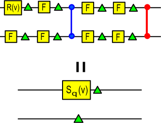
Figure 5: (Color online.) The implementation of $S_{q}(v)\otimes I$. Blue two-qubit gate is $CZ$. Red two-qubit gate is $CZ^{\dagger}$. Green triangles are byproducts.

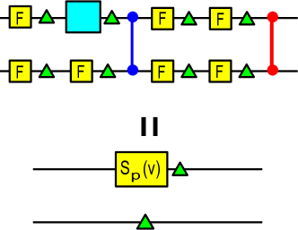
Figure 6: (Color online.) The implementation of $S_{p}(v)\otimes I$. The blue box means $R_{-q}(M_{m}^{-1}v)$.

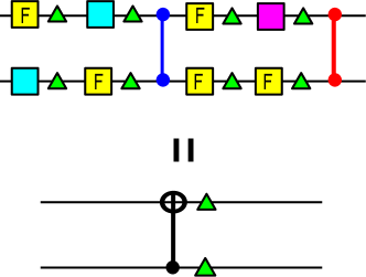
Figure 7: (Color online.) The implementation of $CX$. The blue boxes are $Fe^{iq^{2}/2}$ up to byproduct corrections. The purple box is $Fe^{-iq^{2}/2}$ up to byproduct corrections.

VI Blindness

What Bob obtains are quantum states $\{S_{q}(-\theta_{j})|0\rangle_{p}\}_{j=1}^{N}$ and classical messages $\{\delta_{j}\}_{j=1}^{N}$. Note that

$$\theta_{j} = M_{\xi_{j}}\delta_{j}-\phi_{j}^{\prime}+\eta_{j}e-r_{j}e$$

$$\equiv k_{j}-r_{j}e,$$

where $e=(1,0,0)$. Hence, Bob’s state is

$$\int\prod_{j=1}^{N}dr_{j}\bigotimes_{j=1}^{N}S_{q}(-\theta_{j})|0\rangle_{p}{}_{p}\langle 0|S_{q}^{\dagger}(-\theta_{j})$$

$$= \int\prod_{j=1}^{N}dr_{j}\bigotimes_{j=1}^{N}S_{q}(-k_{j}+r_{j}e)|0\rangle_{p}{}_{p}\langle 0|S_{q}^{\dagger}(-k_{j}+r_{j}e)$$

$$= \int\prod_{j=1}^{N}dr_{j}\bigotimes_{j=1}^{N}S_{q}(-k_{j})e^{ir_{j}q}|0\rangle_{p}{}_{p}\langle 0|e^{-ir_{j}q}S_{q}^{\dagger}(-k_{j})$$

$$= \int\prod_{j=1}^{N}dr_{j}\bigotimes_{j=1}^{N}S_{q}(-k_{j})|r_{j}\rangle_{p}{}_{p}\langle r_{j}|S_{q}^{\dagger}(-k_{j})$$

$$= I^{\otimes N},$$

which means that Bob’s state is independent of $\{\phi_{j}\}_{j=1}^{N}$.

Note that the blindness holds also in the finite squeezed case, since

$$\int\prod_{j=1}^{N}dr_{j}\bigotimes_{j=1}^{N}S_{q}(-\theta_{j})|0,\Omega_{j}\rangle_{p}{}_{p}\langle 0,\Omega_{j}|S_{q}^{\dagger}(-\theta_{j})$$

$$= \int\prod_{j=1}^{N}dr_{j}\bigotimes_{j=1}^{N}S_{q}(-k_{j}+r_{j}e)|0,\Omega_{j}\rangle_{p}{}_{p}\langle 0,\Omega_{j}|S_{q}^{\dagger}(-k_{j}+r_{j}e)$$

$$= \int\prod_{j=1}^{N}dr_{j}\bigotimes_{j=1}^{N}S_{q}(-k_{j})e^{ir_{j}q}|0,\Omega_{j}\rangle_{p}{}_{p}\langle 0,\Omega_{j}|e^{-ir_{j}q}S_{q}^{\dagger}(-k_{j})$$

$$= \int\prod_{j=1}^{N}dr_{j}\bigotimes_{j=1}^{N}S_{q}(-k_{j})e^{ir_{j}q}T_{\Omega_{j}}|0\rangle_{p}{}_{p}\langle 0|T^{\dagger}_{\Omega_{j}}e^{-ir_{j}q}S_{q}^{\dagger}(-k_{j})$$

$$= \int\prod_{j=1}^{N}dr_{j}\bigotimes_{j=1}^{N}T_{\Omega_{j}}\Big{[}S_{q}(-k_{j})e^{ir_{j}q}|0\rangle_{p}{}_{p}\langle 0|e^{-ir_{j}q}S_{q}^{\dagger}(-k_{j})\Big{]}T^{\dagger}_{\Omega_{j}}.$$

Here, the operator

$$T_{\Omega}\equiv\frac{1}{(\pi\Omega^{2})^{1/4}}\int dt~{}~{}e^{-\frac{t^{2}}{2\Omega^{2}}}e^{iqt}$$

commutes with $S_{q}$.

VII Discussion

VII.1 Implementation of $e^{iq^{3}/3}$

In optical systems, the implementation of $e^{iq^{3}/3}$ is much harder than those of $e^{iq}$ and $e^{iq^{2}/2}$. Hence it would be desirable for Alice to avoid the implementation of $e^{iq^{3}/3}$ by herself. There are two solutions. One is that Bob embeds many $e^{isq^{3}/3}|0\rangle_{p}$ with various $s$ into his resource state. If Alice uses the hair implantation technique or the graph hiding technique, Bob cannot know which $e^{isq^{3}/3}|0\rangle_{p}$ contributes to the computation. The other is to use the relation

$$Q^{\dagger}(t)e^{i\gamma q^{3}/3}Q(t)=e^{i\gamma^{\prime}q^{3}/3},$$ (5)

where

$$Q(t)\equiv e^{-i\ln(t)(qp+pq)/2}$$

is the squeezing and $t=(\gamma^{\prime}/\gamma)^{1/3}$. Since the squeezing can be done blindly, Alice can have Bob implement $e^{i\gamma^{\prime}q^{3}/3}$ without allowing Bob to learn $\gamma^{\prime}$.

VII.2 Blind CV protocol for measuring Alice

If the state measurement is relatively easy, we can consider another blind quantum computation protocol, where Bob creates the resource state and Alice does the measurement measuringAlice . One advantage of this protocol is that the security is guaranteed by the no-signaling principle nosignaling , which is more fundamental than quantum physics, and Alice does not need to verify her measurement device (the device independence deviceindependent ). The CV cluster MBQC is suitable for such a measuring Alice protocol, since the measurements of

$$e^{-isq}pe^{isq} = p+s,$$

$$e^{-isq^{2}/2}pe^{isq^{2}/2} = p+sq$$

are easily done with the homodyne detection. The gate $e^{isq^{3}/3}$ can be implemented blindly by using Eq. (5).

VII.3 Temporal encoding

If we use the temporal degrees of freedom, only a single $CZ$ machine is sufficient temporal . As is shown in Fig. 8, it is easy to see that blind versions of such a temporal encoding implementation are possible both for the preparing Alice (Fig. 8 (a)) and the measuring Alice (Fig. 8 (b)).

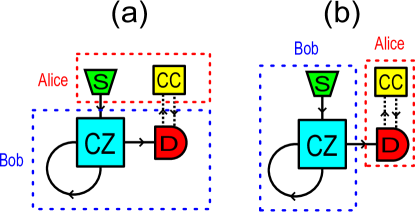
Figure 8: (Color online.) Blind version of the temporal-encoding temporal . S is the squeezed state source, D is the measurement device, CZ is the machine which implements the $CZ$ gate, and CC is a classical computer.

Appendix A Proof of Fig. 5

$$CZ^{\dagger}\left(\begin{array}[]{c}PF\cdot PF\\ PF\cdot PF\end{array}\right)CZ\left(\begin{array}[]{c}PF\cdot PFS_{q}(v)\\ PF\cdot PF\end{array}\right)$$

$$= \left(\begin{array}[]{c}P\\ P\end{array}\right)CZ^{\dagger}\left(\begin{array}[]{c}FF\\ FF\end{array}\right)CZ\left(\begin{array}[]{c}FFS_{q}(v)\\ FF\end{array}\right)$$

$$= \left(\begin{array}[]{c}P\\ P\end{array}\right)CZ^{\dagger}\left(\begin{array}[]{c}FFFF\\ FFFF\end{array}\right)CZ\left(\begin{array}[]{c}S_{q}(v)\\ I\end{array}\right)$$

$$= \left(\begin{array}[]{c}P\\ P\end{array}\right)\left(\begin{array}[]{c}S_{q}(v)\\ I\end{array}\right),$$

where $P$ is a byproduct and

$$CZ^{\dagger}(X(m)\otimes I) = (X(m)\otimes Z(-m))CZ^{\dagger},$$

$$CZ^{\dagger}(I\otimes X(m)) = (Z(-m)\otimes X(m))CZ^{\dagger}.$$

Appendix B Proof of Fig. 6

$$CZ^{\dagger}\left(\begin{array}[]{c}PF\cdot PF\\ PF\cdot PF\end{array}\right)CZ\left(\begin{array}[]{c}PFS_{-q}(M_{m}^{-1}v)\cdot X(m)F\\ PF\cdot PF\end{array}\right)$$

$$= \left(\begin{array}[]{c}P\\ P\end{array}\right)CZ^{\dagger}\left(\begin{array}[]{c}FF\\ FF\end{array}\right)CZ\left(\begin{array}[]{c}FS_{-q}(v)F\\ FF\end{array}\right)$$

$$= \left(\begin{array}[]{c}P\\ P\end{array}\right)CZ^{\dagger}\left(\begin{array}[]{c}FFFF\\ FFFF\end{array}\right)CZ\left(\begin{array}[]{c}S_{p}(v)\\ I\end{array}\right)$$

$$= \left(\begin{array}[]{c}P\\ P\end{array}\right)\left(\begin{array}[]{c}S_{p}(v)\\ I\end{array}\right).$$

Appendix C Proof of Fig. 7

$$CZ^{\dagger}\left(\begin{array}[]{c}X_{g}Fe^{-i(q-h+c+b)^{2}/2}\cdot X_{h}F\\ X_{f}F\cdot X_{e}F\end{array}\right)CZ\left(\begin{array}[]{c}X_{d}Fe^{i(q-c)^{2}/2}\cdot X_{c}F\\ X_{b}F\cdot X_{a}Fe^{iq^{2}/2}\end{array}\right)$$

$$= CZ^{\dagger}\left(\begin{array}[]{c}X_{g}e^{-i(p-h+c+b)^{2}/2}FX_{h}F\\ X_{f}Z_{e}FF\end{array}\right)CZ\left(\begin{array}[]{c}FZ_{-d}X_{c}e^{iq^{2}/2}F\\ FZ_{-b}FZ_{-a}e^{iq^{2}/2}\end{array}\right)$$

$$= CZ^{\dagger}\left(\begin{array}[]{c}X_{g}e^{-i(p-h+c+b)^{2}/2}Z_{h}FF\\ X_{f}Z_{e}FF\end{array}\right)CZ\left(\begin{array}[]{c}FFX_{-d}Z_{-c}e^{ip^{2}/2}\\ FFX_{-b}Z_{-a}e^{iq^{2}/2}\end{array}\right)$$

$$= CZ^{\dagger}\left(\begin{array}[]{c}X_{g}e^{-i(p-h+c+b)^{2}/2}Z_{h}\\ X_{f}Z_{e}\end{array}\right)CZ\left(\begin{array}[]{c}X_{-d}Z_{-c}e^{ip^{2}/2}\\ X_{-b}Z_{-a}e^{iq^{2}/2}\end{array}\right)$$

$$= CZ^{\dagger}\left(\begin{array}[]{c}X_{g}e^{-i(p-h+c+b)^{2}/2}Z_{h}X_{-d}Z_{-c}Z_{-b}\\ X_{f}Z_{e}Z_{-d}X_{-b}Z_{-a}\end{array}\right)CZ\left(\begin{array}[]{c}e^{ip^{2}/2}\\ e^{iq^{2}/2}\end{array}\right)$$

$$= CZ^{\dagger}\left(\begin{array}[]{c}X_{g}Z_{h}X_{-d}Z_{-c}Z_{-b}e^{-ip^{2}/2}\\ X_{f}Z_{e}Z_{-d}X_{-b}Z_{-a}\end{array}\right)CZ\left(\begin{array}[]{c}e^{ip^{2}/2}\\ e^{iq^{2}/2}\end{array}\right)$$

$$= \left(\begin{array}[]{c}P\\ P\end{array}\right)CZ^{\dagger}\left(\begin{array}[]{c}e^{-ip^{2}/2}\\ I\end{array}\right)CZ\left(\begin{array}[]{c}e^{ip^{2}/2}\\ e^{iq^{2}/2}\end{array}\right)$$

$$= \left(\begin{array}[]{c}P\\ P\end{array}\right)CX,$$

where

$$(e^{-ip^{2}/2}\otimes I)e^{iq\otimes q}(e^{ip^{2}/2}\otimes I) = e^{i(q\otimes q)-i(p\otimes q)}$$

$$= e^{i(q\otimes q)}e^{-i(p\otimes q)}(I\otimes e^{-iq^{2}/2})$$

and we have used $e^{A+B}=e^{A}e^{B}e^{-[A,B]/2}$ which is valid if $[A,[A,B]]=[B,[A,B]]=0$.

References

• (1) A. Childs, Quant. Inf. Compt. 5, 456 (2005).
• (2) P. Arrighi and L. Salvail, Int. J. Quant. Inf. 4, 883 (2006).
• (3) A. Broadbent, J. Fitzsimons, and E. Kashefi, Proceedings of the 50th Annual IEEE Symposium on Foundations of Computer Science 517 (2009).
• (4) D. Aharonov, M. Ben-Or, and E. Eban, Proceedings of Innovations in Computer Science 453 (2010).
• (5) T. Morimae, V. Dunjko, and E. Kashefi, arXiv:1009.3486
• (6) V. Dunjko, E. Kashefi, and A. Leverrier, Phys. Rev. Lett. 108, 200502 (2012).
• (7) S. Barz, E. Kashefi, A. Broadbent, J. F. Fitzsimons, A. Zeilinger, and P. Walther, Science 335, 303 (2012).
• (8) T. Morimae and K. Fujii, Nature Comm. 3, 1036 (2012).
• (9) J. F. Fitzsimons and E. Kashefi, arXiv:1203.5217
• (10) T. Morimae and K. Fujii, arXiv:1201.3966
• (11) R. Raussendorf and H. J. Briegel, Phys. Rev. Lett. 86, 5188 (2001).
• (12) R. Raussendorf, D. E. Browne, and H. J. Briegel, Phys. Rev. A 68, 022312 (2003).
• (13) R. Raussendorf, Ph.D. thesis, Ludwig-Maximillians Universität München (2003).
• (14) I. Affleck, T. Kennedy, E. H. Lieb, and H. Tasaki, Comm. Math. Phys. 115, 477 (1988).
• (15) G. K. Brennen and A. Miyake, Phys. Rev. Lett. 101, 010502 (2008).
• (16) R. Raussendorf and J. Harrington, Phys. Rev. Lett. 98, 190504 (2007).
• (17) R. Raussendorf, J. Harrington, and K. Goyal, New J. Phys. 9, 199 (2007).
• (18) R. Raussendorf, J. Harrington, and K. Goyal, Ann. Phys. 321, 2242 (2006).
• (19) Y. Li, D. E. Browne, L. C. Kwek, R. Raussendorf, and T. C. Wei, Phys. Rev. Lett. 107, 060501 (2011).
• (20) K. Fujii and T. Morimae, Phys. Rev. A 85, 010304(R) (2012).
• (21) N. C. Menicucci, P. van Loock, M. Gu, C. Weedbrook, T. C. Ralph, and M. A. Nielsen, Phys. Rev. Lett. 97, 110501 (2006).
• (22) M. Gu, C. Weedbrook, N. C. Menicucci, T. C. Ralph, and P. van Loock, Phys. Rev. A 79, 062318 (2009).
• (23) C. Weedbrook, S. Pirandola, R. Garcia-Patron, N. J. Cerf, T. C. Ralph, J. H. Shapiro, and S. Lloyd, Rev. Mod. Phys. 84, 621 (2012).
• (24) R. Ukai, S. Yokoyama, J. Yoshikawa, P. van Loock, and A. Furusawa, Phys. Rev. Lett. 107, 250501 (2011).
• (25) Y. Miwa, R. Ukai, J. Yoshikawa, R. Filip, P. van Loock, and A. Furusawa, Phys. Rev. A 82, 032305 (2010).
• (26) R. Ukai, N. Iwata, Y. Shimokawa, S. C. Armstrong, A. Politi, J. Yoshikawa, P. van Loock, and A. Furusawa, Phys. Rev. Lett. 106, 240504 (2011).
• (27) M. Yukawa, R. Ukai, P. van Loock, and A. Furusawa, Phys. Rev. A 78,012301 (2008).
• (28) Y. Miwa, J. Yoshikawa, P. van Loock, and A. Furusawa, Phys. Rev. A 80, 050303(R) (2009).
• (29) S. Lloyd and S. L. Braunstein, Phys. Rev. Lett. 82, 1784 (1999).
• (30) M. Ohliger, K. Kieling, and J. Eisert, Phys. Rev. A 82, 042336 (2010).
• (31) S. Popescu and D. Rohrlich, Found. Phys. 24, 379 (1994).
• (32) A. Acin, N. Brunner, N. Gisin, S. Massar, S. Pironio, and V. Scarani, Phys. Rev. Lett. 98, 230501 (2007).
• (33) N. C. Menicucci, X. Ma, T. C. Ralph, Phys. Rev. Lett. 104, 250503 (2010).