Effects of electron-phonon coupling in the Kondo regime of a two-orbital molecule

Abstract

We study the interplay between strong electron-electron and electron-phonon interactions within a two-orbital molecule coupled to metallic leads, taking into account Holstein-like coupling of a local phonon mode to the molecular charge as well as phonon-mediated interorbital tunneling. By combining canonical transformations with numerical renormalization-group calculations to address the interactions nonperturbatively and on equal footing, we obtain a comprehensive description of the system’s many-body physics in the anti-adiabatic regime where the phonons adjust rapidly to changes in the orbital occupancies, and are thereby able to strongly affect the Kondo physics. The electron-phonon interactions strongly modify the bare orbital energies and the Coulomb repulsion between electrons in the molecule, and tend to inhibit tunneling of electrons between the molecule and the leads. The consequences of these effects are considerably more pronounced when both molecular orbitals lie near the Fermi energy of the leads than when only one orbital is active. In situations where a local moment forms on the molecule, there is a crossover with increasing electron-phonon coupling from a regime of collective Kondo screening of the moment to a limit of local phonon quenching. At low temperatures, this crossover is associated with a rapid increase in the electronic occupancy of the molecule as well as a marked drop in the linear electrical conductance through the single-molecule junction.

I Introduction

Single-molecule junctionsTroisi and Ratner (2006, 2005); Ho (2002); Trilisa et al. (2007) are structures consisting of a single molecule bridging the gap between source and drain electrodes, allowing electronic transport when a bias voltage is applied across the structure. These systems, which manifest a rich variety of experimentally accessible physics in a relatively simple setting,Liu et al. (2011) have attracted much theoretical and experimental effort in connection with molecular electronics.Verdaguer (1996); James and Ratner (2003) A major goal of these efforts has been to take advantage of natural or artificial molecules for technological purposes. Examples of single-molecule junctions encompass, for example, single hydrogen moleculesSmith et al. (2002); Djukic et al. (2005); Khoo et al. (2008) and more complex structures such as $4,4^{\prime}$-bipyridine molecules coupled to metallic nanocontacts.Rauba et al. (2008); Li et al. (2006); Stadler et al. (2005)

An important ingredient in transport through molecular systems is the electron-electron interaction (Coulomb repulsion), the effect of which is greatly enhanced by the spatial confinement of electrons in molecules. Electron-electron (e-e) interactions are known to produce Coulomb blockade phenomenaTans:98 ; Park et al. (2002); Kubatkin et al. (2003) and Kondo correlationsHewson (1993); Nygard:00 ; Park et al. (2002); Liang et al. (2002); Pasupathy:04 at low temperatures. Confined electrons are also known to couple to quantized vibrations (phonons) of the molecules,Jaklevic and Lambe (1966) resulting in important effects on electronic transport,Kirtley et al. (1976); Science.280.1732 ; Park:00 ; Gaudioso et al. (2000); Weig:04 ; Kushmerick et al. (2004) including vibrational side-bands found at finite bias in the Kondo regime.Yu:04 ; Parks:07 ; Fernandez-Torrente:08 Single-molecule junctions therefore provide a valuable opportunity to study charge transfer in systems with strong competing interactions.Galperin et al. (2007); Härtle and Thoss (2011)

It has recently been demonstrated that the energies of the molecular orbitals in a single-molecule junction can be tuned relative to the Fermi energy of the electrodes by varying the voltage applied to a capacitively coupled gate.Song et al. (2009) Similar control has for some time been available in another class of nanoelectronic device: a quantum dot coupled to a two-dimensional electron gas.Goldhaber-Gordon et al. (1998); Jeong et al. (2001) The electrons confined in a quantum dot couple—in most cases quite weakly—to collective vibrations of the dot and its substrate.Roca et al. (1994) In single-molecule devices, by contrast, the confined electrons interact with local vibration modes of the molecule that can produce pronounced changes in the molecular electronic orbitals. Consequently, electron-phonon (e-ph) interactions are expected to play a much more important role in molecules than in quantum dots.

From the theoretical point of view, addressing both e-e and e-ph interactions from first principles is a very complicated task. However, simple effective models can provide good qualitative results, depending on the parameter regime and the method employed to solve the model Hamiltonian.Galperin et al. (2007) For example, the essential physics of certain experimentsPark:00 ; Weig:04 appears to be described by variants of the Anderson-Holstein model, which augments the Anderson modelAnderson:61 for a magnetic impurity in a metallic host with a Holstein couplingHolstein:59 of the impurity charge to a local phonon mode. Variants of the model have been studied since the 1970s in connection with other problemsSimanek:79 ; Ting:80 ; Kaga:80 ; Schonhammer:84 ; Alascio:88 ; Schuttler:88 ; Ostreich:91 ; Hewson:02 ; Jeon:03 ; Zhu:03 ; Lee:04 prior to their application to single-molecule devices.Cornaglia:04 ; Cornaglia:05 ; Paaske:05 ; Mravlje:05 ; Büsser, Martins, and Dagotto ; Mravlje:06 ; Nunez:07 ; Cornaglia:07 ; Mravlje:08 ; Dias:09 Various analytical approximations as well as nonperturbative numerical renormalization-group calculations have shown that in equilibrium, the Holstein coupling reduces the Coulomb repulsion between two electrons in the impurity level, even yielding effective e-e attraction for sufficiently strong e-ph coupling. Increasing the e-ph coupling from zero can produce a smooth crossover from a conventional Kondo effect, involving conduction-band screening of the impurity spin degree of freedom, to a charge Kondo effect in which it is the impurity “isospin” or deviation from half-filling that is quenched by the conduction band. In certain cases, the system may realize the two-channel Kondo effect.Dias:09

Single-molecule devices at finite bias are usually studied via nonequilibrium Keldysh Green’s functions that systematically incorporate the many-body interactions within a system. Although this approach has proved to be the most reliable for calculation of transport properties, the results are highly sensitive to the approximations made. For instance, the equation-of-motion techniqueMonreal et al. (2010) generates a hierarchy of coupled equations for Green’s functions containing $2n$ fermionic operators for $n=1$, $2$, $3$, $\ldots$: a hierarchy that must be decoupled at some level in order to become useful. The most commonly used decoupling scheme is based on a mean-field decomposition of the $n=2$ Green’s functions, leading to the well-known Hubbard I approximation.Hubbard (1963) This approximation give reasonable results for temperatures $T$ above the system’s Kondo temperature $T_{K}$, but as it neglects spin correlations between localized and conduction electrons, it fails in the Kondo regime.

A few years ago, two of us applied the equation-of-motion method decoupled at level $n=2$ to study a single-molecule junction that features phonon-assisted interorbital tunneling.Vernek et al. (2007) However, to capture the physics at $T\lesssim T_{K}$ requires extension of the equation-of-motion hierarchy to higher order, which in most cases is carried out in the limit of infinite Coulomb interaction. The Kondo regime may also be studied via diagrammatic expansion within the non-crossing approximation, which is again most straight forward in the infinite-interaction limit.Goker (2011)

This paper reports the results of an investigation of the Kondo regime of a two-orbital molecule, with focus on situations in which Coulomb interactions are strong but finite. Our model Hamiltonian, which includes both phonon-assisted interorbital tunneling and a Holstein-type coupling between the molecular charge and the displacement of the local phonon mode, may also be used to describe two-level quantum dots or a coupled pair of single-level dots. In order to treat e-e and e-ph interactions on an equal basis, we employ Wilson’s numerical renormalization-group approach,Wilson (1975); KWW:1980 ; Bulla et al. (2008) which provides complete access to the equilibrium behavior and linear response of the system for temperatures all the way to absolute zero. We show that the renormalization of e-e interactions is strongly dependent on the energy difference between the two molecular orbitals. For small interorbital energy differences, the renormalization is significantly enhanced compared with the situation of one active molecular orbital considered in previous work. This enhancement is detrimental for realization of the Kondo effect but improves the prospects for accessing a phonon-dominated regime of effective e-e attraction. A sharp crossover between Kondo and phonon-dominated regimes, which has its origin in a level crossing that occurs when the molecule is isolated from the leads, has signatures in thermodynamic properties and in charge transport through the system.

Understanding the equilibrium and linear-response properties of this model is an important precursor to studies of the nonequilibrium steady state, where e-ph effects are likely to reveal themselves at finite bias.Yu:04 ; Parks:07 ; Fernandez-Torrente:08 Moreover, the model we address can readily be adapted to treat the coupling of a single-molecule junction to electromagnetic radiation, a situation where driven interorbital transitions is likely to be of particular importance.

The rest of the paper is organized as follows: Section II describes our model system and provides a preliminary analysis via canonical transformations. Section III reviews the numerical solution method and Sec. IV presents and analyzes results for cases of large and small energy differences between the two molecular orbitals. The main results are summarized in Sec. V.

II Model and Preliminary Analysis

II.1 Model Hamiltonian

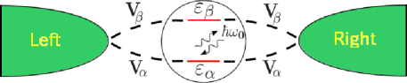
Figure 1: (Color online) Schematic representation of the model studied in this work. A molecule with two active orbitals ($\alpha$ and $\beta$) spans the gap between left and right electrodes. The molecular orbitals are subject both to e-e and e-ph interactions.

We consider a system composed of a two-orbital molecule interacting with a local phonon mode and also coupled to two metallic leads, as shown schematically in Fig. 1. This system is modeled by the Anderson-type Hamiltonian

$$H=H_{\mathrm{mol}}+H_{\mathrm{leads}}+H_{\mathrm{mol-leads}},$$ (1)

with $H_{\mathrm{mol}}$ describing the isolated molecule, $H_{\mathrm{leads}}$ modeling the leads, and $H_{\mathrm{mol-leads}}$ accounting for electron tunneling between the molecule and the leads.

The molecular Hamiltonian can in turn be divided into four parts: $H_{\mathrm{mol}}=H_{\mathrm{e}}+H_{\mathrm{ph}}+H_{\mathrm{Hol}}+H_{\mathrm{tun}}$. Here, the electronic part

$$H_{\mathrm{e}}=\sum_{i=\alpha,\beta}\Bigl{(}\varepsilon_{i}n_{i}+U_{i}n_{i\uparrow}n_{i\downarrow}\Bigr{)}+U^{\prime}n_{\alpha}n_{\beta},$$ (2)

where $n_{i\sigma}=d_{i\sigma}^{{\dagger}}d_{i\sigma}^{\phantom{{\dagger}}}$ is the number operator for electrons of energy $\varepsilon_{i}$ and spin $\sigma$ in molecular orbital $i=\alpha$ or $\beta$, $n_{i}=n_{i\uparrow}+n_{i\downarrow}$, and $U_{i}$ and $U^{\prime}$ parametrize intraorbital and interorbital Coulomb repulsion, respectively. Without loss of generality, we take $\varepsilon_{\beta}\geq\varepsilon_{\alpha}$. The phonon part

$$H_{\mathrm{ph}}=\hbar\omega_{0}\>n_{b}$$ (3)

describes a dispersionless optical phonon mode of energy $\hbar\omega_{0}$, with $n_{b}=b^{{\dagger}}b$. The remaining two parts of $H_{\mathrm{mol}}$ describe two different types of e-ph interaction:

$$H_{\mathrm{Hol}}=\lambda n_{\mathrm{mol}}\bigl{(}b^{{\dagger}}+b\bigr{)}$$ (4)

is a Holstein coupling between the phonon displacement and the combined occupancy (i.e., charge)

$$n_{\mathrm{mol}}=n_{\alpha}+n_{\beta}$$ (5)

of the two molecular orbitals, while

$$H_{\mathrm{tun}}=\lambda^{\prime}\sum_{\sigma}\Bigl{(}d_{\alpha\sigma}^{{\dagger}}d_{\beta\sigma}^{\phantom{{\dagger}}}+d_{\beta\sigma}^{{\dagger}}d_{\alpha\sigma}^{\phantom{{\dagger}}}\Bigr{)}\bigl{(}b^{{\dagger}}+b\bigr{)}$$ (6)

describes interorbital tunneling accompanied by emission or absorption of a phonon. Without loss of generality, we take $\lambda\geq 0$ (since a negative sign can be absorbed into a redefinition of the operator $b$), but we allow $\lambda^{\prime}$ to be of either sign.

The left ($\ell=L$) and right ($\ell=R$) leads are represented by

$$H_{\mathrm{leads}}=\sum_{\ell,\mathbf{k},\sigma}\varepsilon_{\mathbf{k}}c_{\ell\mathbf{k}\sigma}^{{\dagger}}c_{\ell\mathbf{k}\sigma}^{\phantom{{\dagger}}},$$ (7)

where $c_{\ell\mathbf{k}\sigma}$ annihilates an electron with energy $\varepsilon_{\mathbf{k}}$, wave vector $\mathbf{k}$, and spin $\sigma$ in lead $\ell$. For simplicity, each lead is characterized by a flat density of states

$$\rho(\varepsilon)=N_{s}^{-1}\sum_{\mathbf{k}}\delta(\varepsilon-\varepsilon_{\mathbf{k}})=\frac{1}{2D}\,\Theta(D-|\varepsilon|),$$ (8)

where $N_{s}$ is the number of lattice sites in each lead, $D$ is the half bandwidth and $\Theta(x)$ is the Heaviside function.

Lastly,

$$H_{\mathrm{mol-leads}}=\frac{1}{\sqrt{N_{s}}}\sum_{i=\alpha,\beta}\>\sum_{\ell,\mathbf{k},\sigma}\Bigl{(}V_{\ell i}d_{i\sigma}^{{\dagger}}c_{\ell\mathbf{k}\sigma}^{\phantom{{\dagger}}}+V_{i\ell}c_{\ell\mathbf{k}\sigma}^{{\dagger}}d_{i\sigma}^{\phantom{{\dagger}}}\Bigr{)}$$ (9)

describes tunneling or hybridization between the molecular orbitals and the leads, allowing transport through the system. We assume that the tunneling matrix elements are real and have left-right symmetry so we can write $V_{\ell i}=V_{i\ell}=V_{i}$. Then it is useful to perform an even/odd transformation

$$c_{e\mathbf{k}\sigma} =\frac{1}{\sqrt{2}}\bigl{(}c_{R\mathbf{k}\sigma}+c_{L\mathbf{k}\sigma}\bigr{)}$$ (10)

$$c_{o\mathbf{k}\sigma} =\frac{1}{\sqrt{2}}\bigl{(}c_{R\mathbf{k}\sigma}-c_{L\mathbf{k}\sigma}\bigr{)},$$ (11)

which allows Eq. (9) to be rewritten

$$H_{\mathrm{mol-leads}}=\sqrt{\frac{2}{N_{s}}}\sum_{i=\alpha,\beta}V_{i}\sum_{\mathbf{k},\sigma}\Bigl{(}d_{i\sigma}^{{\dagger}}c_{e\mathbf{k}\sigma}^{\phantom{{\dagger}}}+c_{e\mathbf{k}\sigma}^{{\dagger}}d^{\phantom{{\dagger}}}_{i\sigma}\Bigr{)},$$ (12)

With this transformation, the odd-parity degrees of freedom are fully decoupled from the molecular orbitals, and can safely be dropped. As a result, the problem reduces to one effective conduction channel described by a modified

$$H_{\mathrm{leads}}=\sum_{\mathbf{k},\sigma}\varepsilon_{\mathbf{k}}c_{e\mathbf{k}\sigma}^{{\dagger}}c_{e\mathbf{k}\sigma}^{\phantom{{\dagger}}}.$$ (13)

This channel is still described by the density of states in Eq. (8), and it imparts to molecular orbital $i$ a width

$$\Gamma_{i}=\pi V_{i}^{2}/D.$$ (14)

A similar transformation to an effective one-channel model can be derived in any situation where the tunneling matrix elements satisfy $V_{L\alpha}V_{R\beta}=V_{L\beta}V_{R\alpha}$, ensuring that both molecular orbitals couple to the same linear combination of left- and right-lead states.

The Hamiltonian (1) may also describe certain quantum-dot systems. In this setting, the “orbitals” $\alpha$ and $\beta$ can be taken to describe either two active levels within a single quantum dot or the sole active level in two different dots that are coupled to the same pair of external leads.

Since the model laid out above contains eleven energy parameters, it is important to consider the relative values of these parameters in real systems. For small molecules containing up to a few hundred atoms, the largest energy scale (apart possibly from the half bandwidth) is the local Coulomb interaction or charging energy, which is generally of order electron volts. In carbon nanotubes, by contrast, the charging energy can be as lowBomze:10 as 3–4 meV. The numerical results presented in Sec. IV were obtained for the special case of equal intraorbital Coulomb repulsions $U_{\alpha}=U_{\beta}=U$ as well as equal orbital hybridizations $V_{\alpha}=V_{\beta}=V$ (and hence orbital broadenings $\Gamma_{\alpha}=\Gamma_{\beta}=\Gamma$). These choices prove convenient for the algebraic analysis carried out in Secs. II.2 and IV, but qualitatively very similar behavior is obtained for more general ratios $U_{\beta}/U_{\alpha}$ and $V_{\beta}/V_{\alpha}$. Most of the numerical data were computed for an intraorbital interaction $U_{\alpha}=U_{\beta}=U=0.5D$ with an interorbital interaction $U^{\prime}$ of similar size. However, we also include a few results for the limiting cases $U=U^{\prime}=0$ and $U=U^{\prime}=5$.

In the limit where one of the molecular orbitals ($\beta$, say) is removed or becomes decoupled from the rest of the system, the Hamiltonian (1) reduces to the Anderson-Holstein Hamiltonian.Simanek:79 ; Ting:80 ; Kaga:80 ; Schonhammer:84 ; Alascio:88 ; Schuttler:88 ; Ostreich:91 ; Hewson:02 ; Jeon:03 ; Zhu:03 ; Lee:04 ; Cornaglia:04 ; Cornaglia:05 It is well-established for this model that the ratio $\hbar\omega_{0}/\Gamma$ is a key quantity governing the interplay between e-ph interactions and the Kondo effect. In the instantaneous or anti-adiabatic regime $\hbar\omega_{0}\gg\Gamma$, the bosons adjust rapidly to any change in the orbital occupancy, leading to polaronic shifts in the orbital energy and in the Coulomb interaction and to exponential suppression of certain virtual tunneling processes. In the adiabatic regime $\hbar\omega_{0}\ll\Gamma$, by contrast, the phonons are unable to adjust on the typical time scale of hybridization events, and therefore have little impact on the Kondo physics. We expect similar behavior in the two-orbital single-molecule junction, and concentrate in this paper solely on the anti-adiabatic regime $U\gg\hbar\omega_{0}\gg\Gamma$.

In most experiments on molecular junctions, both the phonon energyPark:00 ; Heersche:06 ; Fernandez-Torrente:08 ; Franke:12 and the orbital level broadening due to the leadsLiang et al. (2002); Pasupathy:04 ; Yu:04 ; Makarovski:07 ; Fernandez-Torrente:08 have been found to lie in the range 5–100  meV. All our numerical calculations were performed for a phonon energy $\hbar\omega_{0}=0.1D$ and a hybridization matrix element $V=0.075$, yielding an orbital width $\Gamma=\pi V^{2}/D\simeq 0.0177$ and a ratio $\omega_{0}/\Gamma\simeq 6$ that is somewhat larger than—but not out of line with—that found in one of the few experimentsFernandez-Torrente:08 that has clearly observed vibrational effects in the Kondo regime: transport through a single tetracyanoquinodimethane molecule, where $\omega_{0}=41$ meV and $\Gamma=11$–22 meV. Moderate control of both $\Gamma$ and $\omega_{0}$ has been demonstrated in single-molecule break junctions by changing the separation between the two electrodes,Parks:07 so it seems probable that anti-adiabatic regime will be accessible in future experiments.

Two other important energy scales are the e-ph couplings $\lambda$ and $\lambda^{\prime}$ (or, as will be seen below, the corresponding orbital energy shifts $\lambda^{2}/\hbar\omega_{0}$ and $\lambda^{\prime 2}/\hbar\omega_{0}$). We are aware of no direct measurements of e-ph couplings in single-molecule devices. However, first-principles calculations for one particular setup (a 1,4 benzenedithiolate molecule between aluminum electrodes) have yielded values corresponding in our notation to $\lambda^{2}/\omega_{0}$ up to 0.02 at zero bias and up to 0.08 at strong bias.Sergueev:05 On this basis, we believe that it is very reasonable to consider values of $\lambda^{2}/\omega_{0}$ and $\lambda^{\prime 2}/\omega_{0}$ as large as 0.1.

Also important are the orbital energies $\varepsilon_{\alpha}$ and $\varepsilon_{\beta}$. Many experimental setups allow essentially rigid shifts of these energies through tuning of a back-gate voltage, so we consider sweeps of this form in Sec. IV.2. The energy difference $\varepsilon_{\beta}-\varepsilon_{\alpha}$ will vary widely from system to system, but is not so readily susceptible to experimental control.

It is impossible in a paper of this length to attempt a complete exploration of the model’s parameter space. Instead, guided by the preceding discussion of energy scales, we focus on a few representative examples that illustrate interesting and physically relevant regimes of behavior.

II.2 Preliminary analysis via canonical transformation

Insight can be gained into the properties of the two-orbital model by performing a canonical transformation of the Lang-Firsov typeLang and Firsov (1962) from the original Hamiltonian (1) to $\tilde{H}=e^{S_{1}}He^{-S_{1}}$. Following extensive algebra, it can be shown that the choice

$$S_{1}=\frac{\lambda}{\hbar\omega_{0}}n_{\mathrm{mol}}\bigl{(}b^{{\dagger}}-b\bigr{)}$$ (15)

eliminates the Holstein coupling between the local phonons and the molecular electron occupancy [Eq. (4)], leaving a transformed Hamiltonian

$$\tilde{H}=\tilde{H}_{\mathrm{e}}+H_{\mathrm{ph}}+\tilde{H}_{\mathrm{tun}}+H_{\mathrm{leads}}+\tilde{H}_{\mathrm{mol-leads}},$$ (16)

in which $H_{\mathrm{ph}}$ and $H_{\mathrm{leads}}$ remain as given in Eqs. (3) and (13), respectively; $\tilde{H}_{\mathrm{e}}$ has the same form as $H_{\mathrm{e}}$ [Eq. (2)] with the replacements

$$\varepsilon_{i} \to\tilde{\varepsilon}_{i}=\varepsilon_{i}-{\lambda^{2}}/{\hbar\omega_{0}},$$ (17a)

$$U_{i} \to\tilde{U}_{i}=U_{i}-{2\lambda^{2}}/{\hbar\omega_{0}},$$ (17b)

$$U^{\prime} \to\tilde{U^{\prime}}=U^{\prime}-{2\lambda^{2}}/{\hbar\omega_{0}};$$ (17c)

the interorbital tunneling maps to

$$\tilde{H}_{\mathrm{tun}}=\lambda^{\prime}\sum_{\sigma}\bigl{(}d_{\alpha\sigma}^{{\dagger}}d_{\beta\sigma}^{\phantom{{\dagger}}}+d_{\beta\sigma}^{{\dagger}}d_{\alpha\sigma}^{\phantom{{\dagger}}}\bigr{)}\biggl{[}b^{{\dagger}}+b-\frac{2\lambda}{\hbar\omega_{0}}\bigl{(}1+n_{\alpha\bar{\sigma}}+n_{\beta\bar{\sigma}}\bigr{)}\biggr{]}$$ (18)

where $\bar{\sigma}=-\sigma$; and the molecule-leads coupling term becomes

$$\tilde{H}_{\mathrm{mol-leads}}=\sqrt{\frac{2}{N_{s}}}\sum_{i=\alpha,\beta}V_{i}\sum_{\mathbf{k},\sigma}\Bigl{(}B_{\lambda}^{{\dagger}}d_{i\sigma}^{{\dagger}}c_{e\mathbf{k}\sigma}^{\phantom{{\dagger}}}+B_{\lambda}^{\phantom{{\dagger}}}c_{e\mathbf{k}\sigma}^{{\dagger}}d_{i\sigma}^{\phantom{{\dagger}}}\Bigr{)},$$ (19)

with

$$B_{\xi}=\exp\biggl{[}-\frac{\xi}{\hbar\omega_{0}}\bigl{(}b^{{\dagger}}-b\bigr{)}\biggr{]}\equiv B_{-\xi}^{{\dagger}}.$$ (20)

This transformation extends the one applied previously (e.g., see, Ref. Hewson:02, ) to the Anderson-Holstein model. It effectively eliminates the Holstein Hamiltonian term [Eq. (4)] by mapping the local phonon mode to a different displaced oscillator basis for each value of the total molecular occupancy $n_{\mathrm{mol}}$, namely, the basis that minimizes the ground-state energy of $H_{\mathrm{e}}+H_{\mathrm{ph}}+H_{\mathrm{Hol}}$. There are three compensating changes to the Hamiltonian: (1) Shifts in the orbital energies [Eq. (17a)] and, more notably, a reduction in the magnitude—or even a change in the sign—of each e-e interaction within the molecule [Eqs. (17b) and (17c)]. These renormalizations reflect the fact that the Holstein coupling lowers the energy of doubly occupied molecular orbitals relative to singly occupied and empty orbitals. This well-known effect underlies the standard e-ph mechanism for superconductivity. (2) Addition of correlated (molecular-occupation-dependent) interorbital tunneling [the $\lambda$-dependent term in Eq. (18)] to the phonon-assisted tunneling present in the original Hamiltonian. (3) Incorporation into the molecule-leads coupling [Eq. (19)] of operators $B_{\lambda}^{\phantom{{\dagger}}}$ and $B_{\lambda}^{{\dagger}}$ that cause each electron tunneling event to be accompanied by the creation and absorption of a packet of phonons as the local bosonic mode adjusts to the change in the total molecular occupancy $n_{\mathrm{mol}}$.

The effects of the phonon-assisted interorbital tunneling term $H_{\mathrm{tun}}$ can be qualitatively understood by rewriting Eq. (16) in terms of even and odd linear combinations of the $\alpha$ and $\beta$ molecular orbitals:

$$d_{e\sigma}=\frac{1}{\sqrt{2}}\bigl{(}d_{\alpha\sigma}+d_{\beta\sigma}\bigr{)},\quad d_{o\sigma}=\frac{1}{\sqrt{2}}\bigl{(}d_{\alpha\sigma}-d_{\beta\sigma}\bigr{)}.$$ (21)

In this parity basis, Eq. (18) becomes

$$\tilde{H}_{\mathrm{tun}}=\lambda^{\prime}\sum_{\sigma}(n_{e\sigma}-n_{o\sigma})\biggl{[}b^{{\dagger}}+b-\frac{2\lambda}{\hbar\omega_{0}}\bigl{(}1+n_{e\bar{\sigma}}+n_{o\bar{\sigma}}\bigr{)}\biggr{]},$$ (22)

where $n_{p\sigma}=d_{p\sigma}^{{\dagger}}d_{p\sigma}^{\phantom{{\dagger}}}$ for $p=e$ or $o$. The phonon-assisted tunneling component of $\tilde{H}_{\mathrm{tun}}$ (i.e., the original $H_{\mathrm{tun}}$) can be eliminated by performing a second Lang-Firsov transformation

$$\hat{H}=e^{S_{2}}\tilde{H}e^{-S_{2}}$$ (23)

with

$$S_{2}=\frac{\lambda^{\prime}}{\hbar\omega_{0}}(n_{e}-n_{o})\bigl{(}b^{{\dagger}}-b\bigr{)},$$ (24)

where $n_{p}=n_{p\uparrow}+n_{p\downarrow}$. Lengthy algebra reveals a transformed Hamiltonian

$$\hat{H}=\hat{H}_{\mathrm{e}}+H_{\mathrm{ph}}+H_{\mathrm{leads}}+\hat{H}_{\mathrm{mol-leads}},$$ (25)

where

$$\hat{H}_{\mathrm{e}} =\sum_{p=e,o}\Bigl{(}\tilde{\varepsilon}_{p}\,n_{p}+\tilde{U}_{p}\,n_{p\uparrow}n_{p\downarrow}\Bigr{)}+\sum_{\sigma}\Bigl{(}\tilde{U}_{\parallel}\,n_{e\sigma}n_{o\sigma}+\tilde{U}_{\!\perp}\,n_{e\sigma}n_{o\bar{\sigma}}\Bigr{)}$$

$$+\sum_{\sigma}\bigl{[}t+W\,(n_{e\bar{\sigma}}+n_{o\bar{\sigma}})\bigr{]}\Bigl{(}B_{2\lambda^{\prime}}^{{\dagger}}d_{e\sigma}^{{\dagger}}d_{o\sigma}^{\phantom{{\dagger}}}+B_{2\lambda^{\prime}}^{\phantom{{\dagger}}}d_{o\sigma}^{{\dagger}}d_{e\sigma}^{\phantom{{\dagger}}}\Bigr{)}$$ (26)

$$+J\,\Bigl{(}S_{e}^{+}S_{o}^{-}+S_{o}^{+}S_{e}^{-}+B_{4\lambda^{\prime}}^{{\dagger}}I_{e}^{+}I_{o}^{-}+B_{4\lambda^{\prime}}^{\phantom{{\dagger}}}I_{e}^{-}I_{o}^{+}\Bigr{)}$$

with $S_{p}^{+}\equiv\bigl{(}S_{p}^{-}\bigr{)}^{{\dagger}}=c_{p\uparrow}^{{\dagger}}c_{p\downarrow}^{\phantom{{\dagger}}}$ and $I_{p}^{+}\equiv\bigl{(}I_{p}^{-}\bigr{)}^{{\dagger}}=c_{p\uparrow}^{{\dagger}}c_{p\downarrow}^{{\dagger}}$ being spin- and charge-raising operators, respectively, and

$$\hat{H}_{\mathrm{mol-leads}}=\frac{2}{\sqrt{N_{s}}}\sum_{p=e,o}V_{p}\sum_{\mathbf{k},\sigma}\Bigl{(}B_{\lambda+\lambda^{\prime}}^{{\dagger}}d_{p\sigma}^{{\dagger}}c_{e\mathbf{k}\sigma}^{\phantom{{\dagger}}}+B_{\lambda+\lambda^{\prime}}^{\phantom{{\dagger}}}c_{e\mathbf{k}\sigma}^{{\dagger}}d_{p\sigma}^{\phantom{{\dagger}}}\Bigr{)}.$$ (27)

The renormalized parameters entering Eqs. (II.2) and (27) are

$$\tilde{\varepsilon}_{p} =\frac{\varepsilon_{\alpha}+\varepsilon_{\beta}}{2}-\frac{\lambda_{p}^{2}}{\hbar\omega_{0}},$$ (28a)

$$\tilde{U}_{p} =\frac{2U^{\prime}+U_{\alpha}+U_{\beta}}{4}-\frac{2\lambda_{p}^{2}}{\hbar\omega_{0}},$$ (28b)

$$\tilde{U}_{\parallel} =U^{\prime}-\frac{2\lambda_{e}\lambda_{o}}{\hbar\omega_{0}},$$ (28c)

$$\tilde{U}_{\!\perp} =\frac{2U^{\prime}+U_{\alpha}+U_{\beta}}{4}-\frac{2\lambda_{e}\lambda_{o}}{\hbar\omega_{0}},$$ (28d)

$$t =\frac{\varepsilon_{\alpha}-\varepsilon_{\beta}}{2},$$ (28e)

$$W =\frac{U_{\alpha}-U_{\beta}}{2},$$ (28f)

$$J =\frac{2U^{\prime}-U_{\alpha}-U_{\beta}}{4},$$ (28g)

$$V_{e,o} =\frac{V_{\alpha}\pm V_{\beta}}{2},$$ (28h)

where

$$\lambda_{e,o}=\lambda\pm\lambda^{\prime}.$$ (29)

Since the e-e interactions are expressed much less compactly in the parity basis than in the original basis of $\alpha$ and $\beta$ orbitals, the elimination of the boson-assisted interorbital tunneling from the Hamiltonian comes at the price of much greater complexity in $\hat{H}_{\mathrm{e}}$ compared to $H_{\mathrm{e}}$ [Eq. (2)] and $\tilde{H}_{\mathrm{e}}$. It is notable, though, that the e-e repulsion between two electrons within the even-parity [odd-parity] molecular orbital undergoes a non-negative reduction proportional to $\lambda_{e}^{2}=(\lambda+\lambda^{\prime})^{2}$ [$\lambda_{o}^{2}=(\lambda-\lambda^{\prime})^{2}$]. By contrast, the Coulomb repulsion between electrons in orbitals of different parity undergoes a shift proportional to $-\lambda_{e}\lambda_{o}=\lambda^{\prime 2}-\lambda^{2}$ that may be of either sign. Whereas large values of $\lambda$ favor double occupancy of both the $\alpha$ and the $\beta$ molecular orbital, large values of $|\lambda^{\prime}|$ favor double occupancy of either the $e$ or the $o$ linear combination [the degeneracy between these alternatives being broken by an amount $(2\tilde{\varepsilon}_{e}+\tilde{U}_{e})-(2\tilde{\varepsilon}_{o}+\tilde{U}_{o})=-16\lambda\lambda^{\prime}/\hbar\omega_{0}$]. Both limits yield a unique many-body ground state of a very different character than the spin-singlet Kondo state.

Since $S_{1}$ defined in Eq. (15) can be rewritten $S_{1}=(\lambda/\hbar\omega_{0})(n_{e}+n_{o})\bigl{(}b^{{\dagger}}-b\bigr{)}$, it commutes with $S_{2}$ given in Eq. (24). As a result, the two Lang-Firsov transformations can be combined into a single canonical transformation

$$\hat{H}=e^{S}He^{-S}$$ (30)

with

$$S=S_{1}+S_{2}=\frac{\lambda_{e}n_{e}+\lambda_{o}n_{o}}{\hbar\omega_{0}}\bigl{(}b^{{\dagger}}-b\bigr{)}.$$ (31)

This canonical transformation maps the original phonon annihilation operator $b$ to

$$\hat{b}=e^{S}be^{-S}=b-\frac{\lambda_{e}n_{e}+\lambda_{o}n_{o}}{\hbar\omega_{0}}.$$ (32)

Since $\hat{b}^{{\dagger}}-\hat{b}=b^{{\dagger}}-b$, Eq. (20) can be rewritten

$$B_{\xi}=\exp\biggl{[}-\frac{\xi}{\hbar\omega_{0}}\bigl{(}\hat{b}^{{\dagger}}-\hat{b}\bigr{)}\biggr{]}.$$ (33)

Thus, the operators $B_{2\lambda^{\prime}}$ and $B_{4\lambda^{\prime}}$ entering Eq. (II.2), as well as $B_{\lambda+\lambda^{\prime}}$ in Eq. (27), can be reinterpreted as leading to changes in the occupation $\hat{n}_{b}\equiv\hat{b}^{{\dagger}}\hat{b}$ of the transformed phonon mode.

If the phonon energy $\hbar\omega_{0}$ were to greatly exceed the thermal energy $k_{B}T$ and all other energy scales within the model, the system’s low-energy states would be characterized by $\langle\hat{n}_{b}\rangle\simeq 0$ or, equivalently,

$$\langle n_{b}\rangle\equiv\langle b^{{\dagger}}b\rangle\simeq\biggl{\langle}\biggl{(}\frac{\lambda_{e}n_{e}+\lambda_{o}n_{o}}{\hbar\omega_{0}}\biggr{)}^{2}\biggr{\rangle}.$$ (34)

Moreover, one could approximate other physical quantities by taking expectation values in the transformed phonon vacuum. This approach, which was pioneered in the treatment of the small-polaron problem,Holstein:59a becomes exact in the anti-adiabatic limit $\omega_{0}\to\infty$. However, the physical limit of greatest interest in the two-orbital molecule is one in which the Coulomb interactions $U_{\alpha}$, $U_{\beta}$, and $U^{\prime}$—and hence quite possibly the couplings $|W|$ and $|J|$ associated with changes in $\hat{n}_{b}$—are larger than $\hbar\omega_{0}$. The applicability to such situations of the approximation $\hat{n}_{b}=0$, and of Eq. (34) in particular, is addressed in Sec. IV.

III Numerical renormalization-group approach

In order to obtain a robust description of the many-body physics of the model, we treat the Hamiltonian (1) using Wilson’s numerical renormalization-group (NRG) method,Wilson (1975); KWW:1980 ; Bulla et al. (2008) as extended to incorporate local bosonic degrees of freedom.Hewson:02 The effective conduction band formed by the even-parity combination of left- and right-lead electrons is divided into logarithmic bins spanning the energy ranges $D\Lambda^{-(m+1)}<\pm\varepsilon<D\Lambda^{-m}$ for $m=1$, $2$, $3$, $\ldots$, for some discretization parameter $\Lambda>1$. After the continuum of band states within each bin is approximated by a single representative state (the linear combination of states within the bin that couples to the molecular orbitals), Eq. (13) is mapped via a Lanczos transformation to

$$H_{\mathrm{leads}}\simeq\sum_{n=0}^{\infty}\sum_{\sigma}\tau_{n}\bigl{(}f^{{\dagger}}_{n\sigma}f^{\phantom{{\dagger}}}_{n+1,\sigma}+f^{{\dagger}}_{n+1,\sigma}f^{\phantom{{\dagger}}}_{n\sigma}\bigr{)},$$ (35)

representing a semi-infinite, nearest-neighbor tight-binding chain to which the impurity couples only at its end site $n=0$. Since the hopping decays exponentially along the chain as $\tau_{n}\sim D\Lambda^{-n/2}$, the ground state can be obtained via an iterative procedure in which iteration $N$ involves diagonalization of a finite chain spanning sites $n\leq N$. At the end of iteration $N$, a pre-determined number of low-lying many-body eigenstates is retained to form the basis for iteration $N+1$, thereby allowing reliable access to the low-lying spectrum of chains containing tens or even hundreds of sites. See Ref. Bulla et al., 2008 for general details of the NRG procedure.

For our problem, NRG iteration $N=0$ treats a Hamiltonian $H_{0}=H_{\mathrm{mol}}+H_{\mathrm{mol-leads}}$, with $N_{s}^{-1/2}\sum_{\mathbf{k}}c_{e\mathbf{k}\sigma}$ in Eq. (12) replaced by $\sqrt{2}f_{0\sigma}$. Since the phonon mode described by $H_{\mathrm{ph}}$ has an infinite-dimensional Hilbert space, we must work in a truncated space in which the boson number is restricted to $n_{b}\leq N_{b}$.

III.1 Thermodynamic quantities

The NRG method can be used to evaluate a thermodynamic property $X$ as

$$X(T)=\frac{1}{Z(T)}\sum_{m}\langle\Psi_{m}|X|\Psi_{m}\rangle\>e^{-\beta E_{m}},$$ (36)

where $|\Psi_{m}\rangle$ is a many-body eigenstate at iteration $N$ having energy $E_{m}$, $\beta=1/k_{B}T$, and

$$Z(T)=\sum_{m}e^{-\beta E_{m}}$$ (37)

is the partition function evaluated at the same iteration. For a given value of $N$, Eqs. (36) and (37) provide a good accountWilson (1975); KWW:1980 ; Bulla et al. (2008) of $X(T)$ over a range of temperatures around $T_{N}$ defined by $k_{B}T_{N}=D\Lambda^{-N/2}$.

For extensive properties $X$, it is useful to define the molecular contribution to the property as

$$X_{\mathrm{mol}}=X_{\mathrm{tot}}-X_{\mathrm{leads}},$$ (38)

where $X_{\mathrm{tot}}$ ($X_{\mathrm{leads}}$) is the total value of $X$ for a system with (without) the molecule. In our problem, the local phonon mode is treated as part of the host system. Accordingly, we define the molecular entropy as

$$S_{\!\mathrm{mol}}(T)=S_{\!\mathrm{tot}}(T)-S_{\!\mathrm{leads}}(T)-S_{\!\mathrm{ph}}(T),$$ (39)

where $S_{\!\mathrm{tot}}(T)$ is the total entropy of the system, $S_{\!\mathrm{leads}}(T)$ is the contribution of the leads when isolated from the molecule, and $S_{\!\mathrm{ph}}(T)$ is the entropy of the truncated local-phonon system, given by

$$S_{\!\mathrm{ph}}(T)=k_{B}\bigl{[}\ln Z_{\mathrm{ph}}(T)-\partial\ln Z_{\mathrm{ph}}/\partial\beta\bigr{]},$$ (40)

with

$$Z_{\mathrm{ph}}(T)=\sum_{n_{b}=0}^{N_{b}}e^{-n_{b}\beta\hbar\omega_{0}}=\frac{1-e^{-\beta\hbar\omega_{0}(N_{b}+1)}}{1-e^{-\beta\hbar\omega_{0}}}.$$ (41)

Another property of interest is the molecular contribution to the static magnetic susceptibility,

$$\chi(T)=\frac{\beta(g\mu_{B})^{2}}{Z(T)}\sum_{m}\Bigl{[}\langle\Psi_{m}|S_{z}^{2}|\Psi_{m}\rangle-|\langle\Psi_{m}|S_{z}|\Psi_{m}\rangle|^{2}\Bigr{]}e^{-\beta E_{m}},$$ (42)

where $S_{z}$ is the total spin $z$ operator, $\mu_{B}$ is the Bohr magneton, and $g$ is the Landé g factor (assumed to be the same for electrons in the leads and in the molecular orbitals). One can interpret $|\bm{\mu}_{\mathrm{mol}}|^{2}=3Tk_{B}\chi_{\mathrm{mol}}$ as the magnitude-squared of the molecule’s effective magnetic moment.

III.2 Linear-response transport properties

In this paper, we restrict our calculations to equilibrium situations in which no external bias is applied. In such cases, inelastic transport produced by the e-ph interaction can be neglectedJ.Phys.:Condens.Matter.4.5309 and the linear conductance through the molecule can be obtained from a Landauer-type formula

$$G(T)=G_{0}\int_{-\infty}^{\infty}\biggl{(}-\frac{\partial f}{\partial\omega}\biggr{)}\>\bigl{[}-\mathrm{Im}\,\mathcal{T}(\omega,T)\bigr{]}\>d\omega,$$ (43)

where

$$\mathcal{T}(\omega,T)=\frac{\pi}{2D}\,\sum_{i=\alpha,\beta}\sum_{\sigma}V_{Li}\,G^{\,\sigma}_{ij}(\omega,T)\,V_{jR}.$$ (44)

and $G_{0}=2e^{2}/h$ is the quantum of conductance. The fully dressed retarded molecular Green’s functions $G^{\,\sigma}_{ij}(\omega,T)$ are defined by

$$G^{\,\sigma}_{ij}(\omega,T)=-i\int_{0}^{\infty}\Bigl{\langle}\Bigl{[}d_{i\sigma}^{\phantom{{\dagger}}}(t),d_{j\sigma}^{{\dagger}}(0)\Bigr{]}_{+}\Bigr{\rangle}\,e^{i(\omega+i\eta)t}\,dt,$$ (45)

where $\langle\cdots\rangle$ represents the equilibrium average in the grand canonical ensemble and $\eta$ is a positive infinitesimal real number.

As shown for the related problem of two quantum dots connected in common to a pair of metallic leads,Logan:09 in the case $V_{\ell i}=V_{i\ell}=V_{i}$ assumed in the present work, Eq. (43) can be recast in the simpler form

$$G(T)/G_{0}=\pi\,\Gamma_{c}\sum_{\sigma}\int_{-\infty}^{\infty}\biggl{(}-\frac{\partial f}{\partial\omega}\biggr{)}\>A_{cc}^{\,\sigma}(\omega,T)\>d\omega,$$ (46)

where $\Gamma_{c}=\Gamma_{\alpha}+\Gamma_{\beta}$ and $A_{cc}^{\,\sigma}(\omega,T)=\pi^{-1}\mathrm{Im}\,G^{\,\sigma}_{cc}(\omega,T)$ [defined via Eq. (45)] is the spectral function for the current-carrying linear combination of the $\alpha$ and $\beta$ orbitals:

$$d_{c\sigma}=\sum_{i=\alpha,\beta}\sqrt{\Gamma_{i}/\Gamma_{c}}\,d_{i\sigma}.$$ (47)

Within the NRG approach, one can calculate

$$A_{cc}^{\sigma}(\omega,T) =\frac{1}{Z}\sum_{m,m^{\prime}}\bigl{|}\langle\Psi_{m^{\prime}}|d_{c\sigma}^{{\dagger}}|\Psi_{m}\rangle\bigr{|}^{2}\Bigl{(}e^{-\beta E_{m}}+e^{-\beta E_{n^{\prime}}}\Bigr{)}$$

$$\quad\times\,\delta_{T}\bigl{(}\omega-(E_{m^{\prime}}-E_{m})/\hbar\bigr{)},$$ (48)

where $\delta_{T}(\omega)$ is a thermally broadened Dirac delta function.Bulla et al. (2008) We consider only situations where there is no magnetic field, and hence $A_{cc}^{\sigma}(\omega,T)=A_{cc}(\omega,T)$ independent of $\sigma$.

IV Results

This section presents and interprets essentially exact NRG results for the Hamiltonian defined by Eqs. (1)–(6), (12), and (13). We have been guided in our choice of model parameters by the physical considerations laid out at the end of Sec. II.1. We take the half bandwidth $D=1$ as our primary energy scale and adopt units in which $\hbar=k_{B}=g\mu_{B}=1$.

The results shown below were all obtained for the special case of equal orbital hybridizations $V_{\alpha}=V_{\beta}=V$ and equal intraorbital Coulomb repulsions $U_{\alpha}=U_{\beta}=U$. These choices, which simplify algebraic analysis because they lead to $W=0$ in Eq. (II.2) and $V_{o}=0$ in Eq. (27), are not crucial; qualitatively very similar results are obtained in more general cases. Most of the numerical data were computed for equal intraorbital and interorbital interactions $U=U^{\prime}=0.5$. However, we also include results for other values of $U^{\prime}/U$ and for the limiting cases $U=U^{\prime}=0$ and $U=U^{\prime}=5$.

Our calculations were performed for phonon energy $\omega_{0}=0.1$ and hybridization $V=0.075$, resulting in an orbital width $\Gamma=\pi V^{2}/D\simeq 0.0177$. As discussed in Sec. II.1, the resulting ratio $\omega_{0}/\Gamma\simeq 6$ places the system in the anti-adiabatic regime of greatest interest from the perspective of competition between e-e and e-ph effects. For this fixed value of $\omega_{0}/\Gamma$, we show the consequences of changing the e-ph couplings (a variation of theoretical interest that may be impractical in experiments) and the orbital energies (which can likely be achieved by tuning gate voltages).

Finally, all calculations were performed using an NRG discretization parameter $\Lambda=2.5$, allowing up to $N_{b}=60$ phonons in the local mode, and retaining 2 000–4 000 many-body states after each iteration. These choices are sufficient to reduce NRG discretization and truncation errors to minimal levels.

IV.1 Large orbital energy separation $\varepsilon_{\beta}-\varepsilon_{\alpha}$

We first consider the case of fixed $\varepsilon_{\beta}=4$ where the upper molecular orbital lies far above the chemical potential of the leads and therefore contributes little to the low-energy physics. This situation, in which the two-orbital model largely reduces to the Anderson-Holstein model,Simanek:79 ; Ting:80 ; Kaga:80 ; Schonhammer:84 ; Alascio:88 ; Schuttler:88 ; Ostreich:91 ; Hewson:02 ; Jeon:03 ; Zhu:03 ; Lee:04 ; Cornaglia:04 ; Cornaglia:05 serves as a benchmark against which to compare cases in which both molecular orbitals are active.

Given that the $\beta$ orbital will have negligible occupation, the interorbital Coulomb repulsion $U^{\prime}$ entering $H_{\mathrm{e}}$ [Eq. (2)] and the interorbital e-ph coupling $\lambda^{\prime}$ entering $H_{\mathrm{tun}}$ [Eq. (6)] are not expected to greatly affect the low-energy properties. Throughout this subsection we assume $U^{\prime}=U$ to reduce the number of different parameters that must be specified. Figures 2–5 present results obtained for $\lambda^{\prime}=\lambda$; switching to $\lambda^{\prime}=-\lambda$ would interchange the roles of the even and odd linear combinations of molecular orbitals, but would not change any of the physical quantities shown. Figures 6 and 4 demonstrate that very similar properties arise for $\lambda^{\prime}=0$.

IV.1.1 Isolated molecule

We begin by using the transformed Hamiltonian $\tilde{H}$ defined in Eq. (16) to find analytical expressions for the energies of the low-lying states of the isolated molecule in the absence of any electron tunneling to/from the leads (i.e., for $V=0$). In the regime where $\tilde{\varepsilon}_{\beta}$ is the largest energy scale of the molecule, $\lambda^{\prime}$ manifests itself primarily through perturbative corrections to the energies of the molecule when the $\alpha$ orbital is occupied by $n_{\mathrm{mol}}=0$, $1$, or $2$ electrons.

Let us focus on the state of lowest energy in each occupancy sector. This is the state having zero occupancy of the transformed boson mode entering the Hamiltonian $\tilde{H}$, whose energy we will denote $E^{(n_{\mathrm{mol}})}_{\min}$. The empty molecule is unaffected by the interorbital e-ph coupling, so $E^{(0)}_{\min}=0$. To second order in $\tilde{H}_{\mathrm{tun}}$ defined in Eq. (18),

$$E^{(1)}_{\min}\equiv\tilde{\tilde{\varepsilon}}_{\alpha} =\tilde{\varepsilon}_{\alpha}-\frac{\lambda^{\prime 2}}{\tilde{\varepsilon}_{\beta}-\tilde{\varepsilon}_{\alpha}+\omega_{0}}-\biggl{(}\frac{2\lambda}{\omega_{0}}\biggr{)}^{2}\frac{\lambda^{\prime 2}}{\tilde{\varepsilon}_{\beta}-\tilde{\varepsilon}_{\alpha}}$$

$$\simeq\varepsilon_{\alpha}-\lambda^{2}/\omega_{0}-(1+4\lambda^{2}/\omega_{0}^{2})\>\lambda^{\prime 2}/\varepsilon_{\beta},$$ (49)

where in the second expression we have used $\tilde{\varepsilon}_{\beta}-\tilde{\varepsilon}_{\alpha}=\varepsilon_{\beta}-\varepsilon_{\alpha}$. In the same approximation, the energy of the doubly occupied molecule becomes

$$E^{(2)}_{\min} =2\tilde{\varepsilon}_{\alpha}+\tilde{U}_{\alpha}-\frac{2\lambda^{\prime 2}}{\tilde{\varepsilon}_{\beta}-\tilde{\varepsilon}_{\alpha}+\tilde{U}^{\prime}-\tilde{U}_{\alpha}+\omega_{0}}$$

$$\qquad-\biggl{(}\frac{4\lambda}{\omega_{0}}\biggr{)}^{2}\frac{2\lambda^{\prime 2}}{\tilde{\varepsilon}_{\beta}-\tilde{\varepsilon}_{\alpha}+\tilde{U}^{\prime}-\tilde{U}_{\alpha}}$$

$$\simeq 2\tilde{\varepsilon}_{\alpha}+\tilde{U}-2(1+16\lambda^{2}/\omega_{0}^{2})\>\lambda^{\prime 2}/\varepsilon_{\beta}$$ (50)

in the case $U_{\alpha}=U^{\prime}=U$ considered throughout this discussion of large orbital separation. Equations (IV.1.1) and (IV.1.1) allow us to define an effective interaction within the $\alpha$ orbital

$$\tilde{\tilde{U}}_{\alpha}=E^{(2)}_{\min}-2E^{(1)}_{\min}=U-2\lambda^{2}/\omega_{0}-24(\lambda^{2}/\omega_{0}^{2})\>\lambda^{\prime 2}/\varepsilon_{\beta}.$$ (51)

For future reference, we also define

$$\Delta E_{12}=E^{(1)}_{\min}-E^{(2)}_{\min}=3\lambda^{2}/\omega_{0}+(1+28\lambda^{2}/\omega_{0}^{2})\,\lambda^{\prime 2}/\varepsilon_{\beta}-\varepsilon_{\alpha}-U.$$ (52)

The ground state of the isolated molecule lies in the sector of occupancy $n_{\mathrm{mol}}$ having the smallest value of $E^{(n_{\mathrm{mol}})}_{\min}$. Under variation of a molecular parameter such as $\varepsilon_{\alpha}$ or $\lambda$, a jump will occur between $n_{\mathrm{mol}}=0$ and 1 at any point where $E^{(1)}_{\min}=0<E^{(2)}_{\min}$, between $n_{\mathrm{mol}}=1$ and 2 where $E^{(2)}_{\min}=E^{(1)}_{\min}<0$, and directly between $n_{\mathrm{mol}}=0$ and 2 where $E^{(2)}_{\min}=0<E^{(1)}_{\min}$. In the presence of a small level width $\Gamma>0$, one expects these jumps to be broadened into smooth crossovers centered at points in parameter space close to their locations for the isolated molecule.

IV.1.2 Effect of varying the lower orbital energy

Now we turn to numerical solutions of the full problem with $\varepsilon_{\beta}=4$, a dot-lead hybridization $V=0.075$, and a phonon energy $\omega_{0}=0.1$. In this subsection we examine the effect of varying the energy $\varepsilon_{\alpha}$ of the lower molecular orbital at $T=0$.

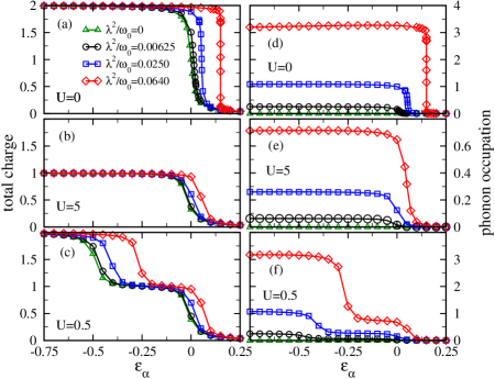
Figure 2: (Color online) Variation with orbital energy $\varepsilon_{\alpha}$ at zero temperature of (left) the charge $\langle n_{\mathrm{mol}}\rangle$, and (right) the phonon occupation $\langle n_{b}\rangle$, for $U=0$ (top), $U=5$ (middle) and $U=0.5$ (bottom). Data are for $\varepsilon_{\beta}=4$, $U^{\prime}=U$, $\lambda^{\prime}=\lambda$, and the four values of $\lambda^{2}/\omega_{0}$ listed in the legend.

Figure 2 shows the total molecular charge $\langle n_{\mathrm{mol}}\rangle$ and the occupation $\langle n_{b}\rangle$ of the original phonon mode [as opposed to the occupation $\langle\hat{n}_{b}\rangle$ of the transformed mode defined in Eq. (32)] as functions of $\varepsilon_{\alpha}$ for four values of $\lambda$ and three values of $U$. First consider the case $U=0$ of vanishing e-e interactions shown in panels (a) and (d). For $\lambda=\lambda^{\prime}=0$, $\varepsilon_{\alpha}=0$ is a point of degeneracy between configurations having molecular charges 0, 1, and 2; $\langle n_{\mathrm{mol}}\rangle$ increases from 0 to 2 over a narrow range $\Delta\varepsilon_{\alpha}\simeq 4\Gamma$ as the $\alpha$ orbital drops below the chemical potential of the leads. For $\lambda>0$, $\tilde{U}=-2\lambda^{2}/\omega_{0}$ is negative, and the ground state switches from charge 0 to charge 2 around the point where $E^{(2)}_{\min}=E^{(0)}_{\min}$ or $\varepsilon_{\alpha}=2\lambda^{2}/\omega_{0}+(1+16\lambda^{2}/\omega_{0}^{2})\,\lambda^{\prime 2}/\varepsilon_{\beta}$. There is a marked decrease with increasing $\lambda$ in the width $\Delta\varepsilon_{\alpha}$ of the region of rapid change in the charge. (We will henceforth refer to such a measure as the “rise width” to avoid possible confusion with the width of the plateau between two successive rises.)

It is evident from Figs. 2(a) and 2(d) that changes in the ground-state phonon occupation are closely correlated with those in the total molecular charge. The prediction of Eq. (34) for the case $\lambda^{\prime}=\lambda$ (hence, $\lambda_{e}=2\lambda$ and $\lambda_{o}=0$) is $\langle n_{b}\rangle=(2\lambda/\omega_{0})^{2}\,\langle n_{e}^{2}\rangle$. Although this relation captures the correct trends in the variation of $\langle n_{b}\rangle$ with $\varepsilon_{\alpha}$ in Fig. 2(d), it overestimates the phonon occupation by a significant margin. Such deviations are not unexpected, given that Eq. (34) was derived under the assumption that $\hbar\omega_{0}$ is the largest energy scale in the problem, whereas here $\varepsilon_{\beta}$ is the dominant energy scale, followed by $U=U^{\prime}$. Empirically, we find that $\langle n_{b}\rangle$ lies closer to

$$\bar{n}_{b}=(2\lambda/\omega_{0})^{2}\,\langle n_{e}\rangle^{2},$$ (53)

which also serves as an empirical lower bound on the phonon occupation. The error $\langle n_{b}\rangle-\bar{n}_{b}$ is largest in the vicinity of the sharpest rise in $\langle n_{\mathrm{mol}}\rangle$ and vanishes as $\langle n_{\mathrm{mol}}\rangle$ approaches 0 or 2. For $\lambda^{2}/\omega_{0}=0.064$, $\langle n_{b}\rangle-\bar{n}_{b}<0.06$ both for $\varepsilon_{\alpha}\leq 0.149$ and for $\varepsilon_{\alpha}\geq 0.151$, whereas for $\varepsilon_{\alpha}=0.149945$, $\bar{n}_{b}\simeq 0.88$ underestimates $\langle n_{b}\rangle$ by approximately $0.68$. The peak error is smaller for the other e-ph couplings shown in Fig. 2(d).

For the case $U=5$ of very strong e-e interactions [Fig. 2(b) and 2(e)], the molecular charge rises from 0 to 1 around the point where $E^{(1)}_{\min}=E^{(0)}_{\min}$ or $\varepsilon_{\alpha}\simeq 2\lambda^{2}/\omega_{0}+(1+4\lambda^{2}/\omega_{0}^{2})\,\lambda^{\prime 2}/\varepsilon_{\beta}$. In contrast with the situation for $U=0$, the rise width $\Delta\varepsilon_{\alpha}$ shows no appreciable change with $\lambda$. The phonon occupation is described by Eq. (53) even better than for $U=0$, with the greatest error ($\langle n_{b}\rangle-\bar{n}_{b}\simeq 0.08$ for $\lambda^{2}/\omega_{0}=0.064$) occurring around the point where $\langle n_{\mathrm{mol}}\rangle=0.5$.

Lastly, Figs. 2(c) and 2(f) show data for $U=0.5$, exemplifying moderately strong e-e interactions. With decreasing $\varepsilon_{\alpha}$ (at fixed $\lambda$), the molecular charge rises in two steps, first rising from 0 to 1 as $E^{(1)}_{\min}$ falls below $E^{(0)}_{\min}$, and then rising from 1 to 2 as $E^{(1)}_{\min}$ in turn falls below $E^{(2)}_{\min}$ at [see Eq. (52)]

$$\varepsilon_{\alpha}\simeq-U+3\lambda^{2}/\omega_{0}+(1+28\lambda^{2}/\omega_{0}^{2})\,\lambda^{\prime 2}/\varepsilon_{\beta}.$$ (54)

Just as for $U=5$, each rise has a width $\Delta\varepsilon_{\alpha}=O(\Gamma)$ that is independent of $\lambda$ over the range of e-ph couplings shown. The distance along the $\varepsilon_{\alpha}$ axis between the two rises (i.e., the width of the charge-1 plateau) is roughly $\tilde{\tilde{U}}$ defined in Eq. (51), which decreases as the e-ph coupling increases in magnitude. The phonon occupation is again well-approximated by $\bar{n}_{b}$ given in Eq. (53).

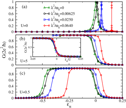
Figure 3: (Color online) Zero-temperature conductance $G$ vs orbital energy $\varepsilon_{\alpha}$ for (a) $U=0$, (b) $U=5$, and (c) $U=0.5$. Data are for $\varepsilon_{\beta}=4$, $U^{\prime}=U$, $\lambda^{\prime}=\lambda$, and the four values of $\lambda^{2}/\omega_{0}$ listed in the legend. The inset in (b) shows the data from the main panel replotted as $G$ vs $\tilde{\varepsilon}_{\alpha}/\tilde{U}$.

Figure 3 plots the zero-temperature linear conductance as a function of $\varepsilon_{\alpha}$ for the same set of parameters as was used in Fig. 2. At $T=0$ in zero magnetic field, Eq. (46) reduces to $G(T=0)/G_{0}=\pi\,\Gamma_{c}A_{cc}(0,0)$. In any regime of Fermi-liquid behavior, $A_{cc}(0,0)$ is expected to obey the Friedel sum-rule, implying that $\pi\,\Gamma_{c}A_{cc}(0,0)=\sin^{2}(\pi\langle n_{\mathrm{mol}}\rangle/2)$ in the wide-band limit where all other energy scales in the model are small compared with $D$. This property, which should hold even in the presence of e-ph interactions within the molecule, leads to

$$G(T=0)=G_{0}\,\sin^{2}\biggl{(}\frac{\pi}{2}\langle n_{\mathrm{mol}}\rangle\biggr{)}\,.$$ (55)

For $U=0$ [Fig. 3(a)], we observe a conductance peak at the point of degeneracy between molecular charges 0 and 2. This is the noninteracting analog of the Coulomb blockade peak seen in strongly interacting quantum dots and single-molecule junctions above their Kondo temperatures. For $\lambda=0$, the peak is located at $\varepsilon_{\alpha}=0$ and has a full width $\Delta\varepsilon_{\alpha}\simeq 2\Gamma$, as expected for this exactly solvable single-particle case. With increasing $\lambda$, the conductance peak shifts to higher $\varepsilon_{\alpha}$ while its width narrows, trends that both follow via Eq. (55) from the behavior of $\langle n_{\mathrm{mol}}\rangle$ in Fig. 2(a). For all values of $\lambda$, the maximum conductance is $G=G_{0}$, as predicted by Eq. (55) for the point where $\langle n_{\mathrm{mol}}\rangle$ passes through $1$.

The sharp features shown in Fig. 3(a) allow one to quantify the accuracy of the approximation of using energies of the isolated molecule in the no-boson state of the transformed phonon mode to locate features in the full system. In the case $\lambda^{2}/\omega_{0}=0.064$, for example, the NRG calculations place the peak in $G$ at $\varepsilon_{\alpha}=0.152$, whereas the criterion $E^{(2)}_{\min}=E^{(0)}_{\min}$ gives $\varepsilon_{\alpha}=2\lambda^{2}/\omega_{0}+(1+16\lambda^{2}/\omega_{0}^{2})\,\lambda^{\prime 2}/\varepsilon_{\beta}=0.162$. Thus, the coupling of the molecule to external leads and the admixture of states with nonzero phonon number produces a downward shift in the peak position of roughly $0.1$, considerably larger than the upward shift $0.018$ predicted to arise from the $\lambda^{\prime}$ interorbital e-ph coupling $\lambda^{\prime}$.

For the interacting cases shown in Figs. 3(b) and 3(c), the formation of a many-body Kondo resonance at the chemical potential leads to a near-unitary conductance at low-temperatures $T\ll T_{K}$ over the entire range of $\varepsilon_{\alpha}$ for which $\langle n_{\mathrm{mol}}\rangle\simeq 1$. In the case $U=5$, no data are shown for $\varepsilon_{\alpha}\lesssim-0.4$, a range in which the Kondo temperature $T_{K}$ is so low that the ground-state properties are experimentally inaccessible. For both nonzero values of $U$, the width of each conductance rise is independent of $\lambda$ over the range of e-ph couplings shown.

The narrowing with increasing $\lambda$ of the rises in the molecular charge and the phonon occupancy, and of the peaks in the linear conductance, seen for $U=0$ but not in the data presented for $U=0.5$ or $U=5$, is associated with the presence of a crossover of $\langle n_{\mathrm{mol}}\rangle$ directly from 0 to 2. Similar narrowing is, in fact, seen for $U>0$ when $\lambda$ become sufficiently large to suppress the $\langle n_{\mathrm{mol}}\rangle=1$ plateau. (In the case $U=0.5$ and $\lambda^{\prime}=\lambda$, this takes place around $\lambda^{2}/\omega_{0}=0.15$, considerably larger than any of the values shown in Figs. 2 and 3.) This phenomenon is known from the Anderson-Holstein model (e.g., see Ref. Cornaglia:04, ) to arise from the small overlap between the bosonic ground state of the displaced oscillator that minimizes the energy in the sectors $n_{\mathrm{mol}}=0$ and the corresponding ground state for $n_{\mathrm{mol}}=2$. This small overlap leads to an exponential reduction in the effective value of the level width $\Gamma$ in the regime of negative effective $U$.

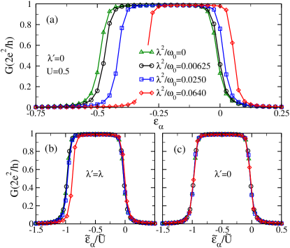
Figure 4: (Color online) (a) Zero-temperature conductance $G$ vs orbital energy $\varepsilon_{\alpha}$ for the same parameters as used in Fig. 3(c), except here $\lambda^{\prime}=0$. (b) Data for $\lambda^{\prime}=\lambda$ from Fig. 3(c) replotted as $G$ vs $\tilde{\varepsilon}_{\alpha}/\tilde{U}$. (c) Data for $\lambda^{\prime}=0$ from (a) replotted as $G$ vs $\tilde{\varepsilon}_{\alpha}/\tilde{U}$.

It has already been remarked that the phonon-assisted interorbital tunneling is expected to play only a minor role in cases where the $\beta$ orbital is far above the Fermi energy. To test this expectation, we have compared data for $\lambda^{\prime}=\lambda$ and $\lambda^{\prime}=0$ with all other parameters the same. The conductance curves in the two cases are also similar, as exemplified for $U=0.5$ by Figs. 3(c) and 4(a). The same conclusion holds for the molecular charge and phonon occupation (data for $\lambda^{\prime}=0$ not shown). However, there are subtle differences that can be highlighted by replotting properties as functions of the scaling variable $\tilde{\varepsilon}_{\alpha}/\tilde{U}$. For example, the conductance data for $\lambda^{\prime}=0$ and $U=0.5$ show almost perfect collapse [Fig. 4(c)], confirming that in this case the conductance rises are centered close to $\tilde{\varepsilon}_{\alpha}=0$ and $\tilde{\varepsilon}_{\alpha}=-\tilde{U}$, the values predicted based on the low-lying levels of the isolated molecule. For $\lambda^{\prime}=\lambda$, the data collapse [shown in Fig. 4(b) for $U=0.5$, and in the inset to Fig. 3(b) for $U=5$] is good for small values of $\lambda$ but less so for $\lambda^{2}/\omega_{0}=0.064$, a case where $\tilde{\tilde{\varepsilon}}_{\alpha}$ and $\tilde{\tilde{U}}_{\alpha}$ defined in Eqs. (IV.1.1) and (51) differ appreciably from $\tilde{\varepsilon}_{\alpha}$ and $\tilde{U}$.

IV.1.3 Lower orbital close to chemical potential

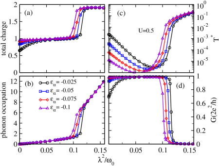
Figure 5: (Color online) Variation with $\lambda^{2}/\omega_{0}$ of (a) the ground-state molecular charge $\langle n_{\mathrm{mol}}\rangle$, (b) the ground-state phonon occupation $\langle n_{b}\rangle$, (c) the crossover temperature $T^{*}$, and (d) the zero-temperature linear conductance $G$, all calculated for $U^{\prime}=U=0.5$, $\lambda^{\prime}=\lambda$, $\varepsilon_{\beta}=4$, and the four values of $\varepsilon_{\alpha}$ listed in the legend.

We now switch focus from the variation of properties with $\varepsilon_{\alpha}$ to trends with increasing e-ph coupling. Figure 5(a) shows the evolution of the zero-temperature molecular charge $\langle n_{\mathrm{mol}}\rangle$ with $\lambda^{2}/\omega_{0}$ for $U=U^{\prime}=0.5$, $\lambda^{\prime}=\lambda$, and four different values of $\varepsilon_{\alpha}$. We begin by considering the special case $\lambda=0$ in which the electron and phonon subsystems are entirely decoupled. Here, $\langle n_{\mathrm{mol}}\rangle$ ranges from roughly two-thirds for $\varepsilon_{\alpha}=-0.025$ (an example of mixed valence where the lower molecular orbital lies below the Fermi energy by an amount that barely exceeds $\Gamma=\pi V^{2}/D\simeq 0.0177$) to nearly one for $\varepsilon_{\alpha}=-0.075$ and $-0.1$. In the latter limit, the large Coulomb repulsion $U$ leads to local-moment formation in the $\alpha$ orbital. The local moment is collectively quenched by lead electrons, leading to a Kondo singlet ground state. Figure 5(c) shows the characteristic temperature $T^{*}$ of the quenching of the molecular spin degree of freedom, determined via the standard criterionWilson (1975) $T^{*}\chi_{\mathrm{mol}}(T^{*})=0.0701$. This scale is of order $\Gamma$ deep in the mixed-valence limit (i.e., for $|\varepsilon_{\alpha}|\ll\Gamma$), but is exponentially reduced in the local-moment regime $-\varepsilon_{\alpha}\gg\Gamma$ where it represents the system’s Kondo temperature, given for $U\gg-\varepsilon_{\alpha}\gg\Gamma$ byHaldane:78

$$T_{K}\simeq\sqrt{\Gamma U}\,\exp(\pi\varepsilon_{\alpha}/2\Gamma).$$ (56)

Upon initial increase of $\lambda$, the effective level position $\tilde{\tilde{\varepsilon}}_{\alpha}$ decreases according to Eq. (IV.1.1), the occupancy of the lower molecular orbital (and hence the total occupancy $\langle n_{\mathrm{mol}}\rangle$) rises ever closer to one, and the temperature $T^{*}$ decreases as expected from the replacement of $\varepsilon_{\alpha}$ and $U$ in Eq. (56) by $\tilde{\tilde{\varepsilon}}_{\alpha}$ and $\tilde{\tilde{U}}_{\alpha}$. Neglecting both the subleading $\lambda$ dependence coming from $\tilde{U}$ and the $\lambda^{\prime}$ contributions to $\tilde{\tilde{\varepsilon}}_{\alpha}$, one arrives at the relation

$$T^{*}(\lambda)\simeq T^{*}(0)\>\exp\left[-\pi\lambda^{2}/(2\Gamma\omega_{0})\right],$$ (57)

which accounts quite well for the initial variation of $T^{*}$ in Fig. 5(c).

Upon further increase in the e-ph coupling, $\langle n_{\mathrm{mol}}\rangle$ and $T^{*}$ both show rapid but continuous rises around some value $\lambda=\lambda_{x}$ that is close to the one predicted by the vanishing of $E^{(2)}_{\min}=E^{(1)}_{\min}$ for the increase from 1 to 2 in the charge of the isolated molecule: solving Eq. (52) with $\Delta E_{12}=0$ to find $\lambda=\lambda^{\prime}$ yields $\lambda_{x}^{2}/\omega_{0}=0.122$, $0.117$, $0.112$, and $0.106$ for $\varepsilon_{\alpha}=-0.025$, $-0.05$, $-0.075$, and $-0.1$, respectively—values close to but slightly above those observed in the full numerical solutions [the magnitude and sign of the small discrepancies being consistent with those noted previously in connection with the $U=0$ data in Fig. 3(a)]. For $\Gamma>0$, the energies corresponding to $E_{1}^{(1)}$ and $E_{1}^{(2)}$ each acquire a half width $\Gamma$, so the crossover of the ground-state molecular charge from 1 to 2 is smeared over the range $|E^{(2)}_{\min}-E^{(1)}_{\min}|\lesssim 2\Gamma$. Solving Eq. (52) again with $\Delta E_{12}=\pm 2\Gamma$ gives the full width for the crossover as $\Delta(\lambda^{2}/\omega_{0})\simeq 0.016$, an estimate in good agreement with the data in Fig. 5(a).

In the regime $\lambda\gtrsim\lambda_{x}$, minimization of the e-ph energy through $\langle n_{\alpha}\rangle\simeq 2$, $\langle n_{\beta}\rangle\simeq 0$ outweighs the benefits of forming a many-body Kondo singlet. Therefore, $T^{*}$ characterizing the vanishing of $T\chi_{\mathrm{mol}}$ ceases to represent the Kondo temperature and instead characterizes the scale, of order $\Delta E_{12}$ defined in Eq. (52), at which $n_{\mathrm{mol}}=1$ spin-doublet molecular states become thermally inaccessible.

Over the entire range of $\delta$ and $\lambda^{2}/\omega_{0}$ illustrated in Fig. 5, the ground-state phonon occupation $\langle n_{b}\rangle$ [Fig. 5(b)] closely tracks $\bar{n}_{b}$ defined in Eq. (53) to within an absolute error $0\leq\langle n_{b}\rangle-\bar{n}_{b}\leq 0.2$, an error that peaks around $\lambda=\lambda_{x}$. Similarly, the $T=0$ conductance [Fig. 5(d)] is everywhere well-described by Eq. (55), reaching the unitary limit $G_{0}$ over a window of Kondo behavior for $\lambda\lesssim\lambda_{x}$ in which the molecular charge is 1, then plunging to zero as the Kondo effect is destroyed and the occupancy rises to 2.

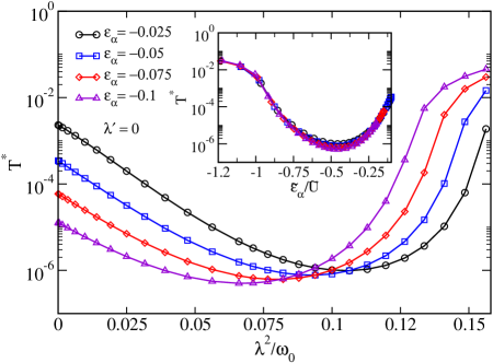
Figure 6: (Color online) Variation with $\lambda^{2}/\omega_{0}$ of the crossover temperature $T^{*}$ calculated for $U^{\prime}=U=0.5$, $\lambda^{\prime}=0$, $\varepsilon_{\beta}=4$, and the four values of $\varepsilon_{\alpha}$ listed in the legend. Inset: The same $T^{*}$ data plotted vs the ratio $\tilde{\varepsilon}_{\alpha}/\tilde{U}_{\alpha}$ of phonon-renormalized molecular parameters.

As another illustration of the effect of relaxing the assumption $\lambda^{\prime}=\lambda$, Fig. 6 shows the variation with $\lambda^{2}/\omega_{0}$ of $T^{*}$, calculated for the same parameters as in Fig. 5(c), except that here $\lambda^{\prime}=0$. For each value of $\varepsilon_{\alpha}$, the variation of $T^{*}$ is very similar in the two cases apart from a considerably larger value of $\lambda_{x}$ for $\lambda^{\prime}=0$, a change that is predicted at the level of the isolated molecule where Eq. (52) with $\lambda^{\prime}=\Delta E_{12}=0$ gives $\lambda_{x}^{2}/\omega_{0}=(U+\varepsilon_{\alpha})/3$, which ranges from $0.158$ for $\varepsilon_{\alpha}=-0.025$ to $0.133$ for $\varepsilon_{\alpha}=-0.1$. Just as seen in Fig. 4(c), the $\lambda^{\prime}=0$ data exhibit excellent collapse when plotted against the ratio $\tilde{\varepsilon}_{\alpha}/\tilde{U}$ of effective molecular parameters defined in Eqs. (17).

IV.2 Small orbital energy separation $\varepsilon_{\beta}-\varepsilon_{\alpha}$

The rich behavior of the model described by Eqs. (1)–(9) becomes apparent only in the regime where the two molecular orbitals lie close in energy so that they can both contribute strongly to the low-energy physics. For simplicity, we focus primarily on situations with equal e-ph couplings $\lambda^{\prime}=\lambda$, equal Coulomb interactions $U^{\prime}=U$, and symmetrical placement of the orbitals with respect to the chemical potential of the leads, i.e., $\varepsilon_{\beta}=-\varepsilon_{\alpha}=\delta$, a small positive energy scale. However, we present results for more general parameter choices at several points throughout the subsection.

IV.2.1 Isolated molecule

$n_{\mathrm{mol}}$	$i$	$|\phi^{(n_{\mathrm{mol}})}_{i}(\delta\!=\!0)\rangle$	$E^{(n_{\mathrm{mol}})}_{i}(\delta\!=\!0)$	$E^{(n_{\mathrm{mol}})}_{i}(\delta\!>\!0)$
$0$	$1$	$|\hat{0}\rangle$	$0$	$0$
$1$	$1$	$d_{e\uparrow}^{{\dagger}}|\hat{0}\rangle$	$-(x\!+\!x^{\prime})^{2}$	$-4x^{2}\!-\!\frac{1}{4}y$
	$2$	$d_{e\downarrow}^{{\dagger}}|\hat{0}\rangle$	$-(x\!+\!x^{\prime})^{2}$	$-4x^{2}\!-\!\frac{1}{4}y$
	$3$	$d_{o\uparrow}^{{\dagger}}|\hat{0}\rangle$	$-(x\!-\!x^{\prime})^{2}$	$\frac{1}{4}y$
	$4$	$d_{o\downarrow}^{{\dagger}}|\hat{0}\rangle$	$-(x\!-\!x^{\prime})^{2}$	$\frac{1}{4}y$
$2$	$1$	$\bigl{(}c_{1}d_{e\uparrow}^{{\dagger}}d_{e\downarrow}^{{\dagger}}\!\!+\!c_{2}d_{o\uparrow}^{{\dagger}}d_{o\downarrow}^{{\dagger}}\bigr{)}|\hat{0}\rangle$	$\bar{U}\!-\!4(x^{2}\!+\!x^{\prime 2})\!-\!\tilde{\Delta}$	$U\!-\!16x^{2}\!-\!\frac{1}{6}y$
	$2$	$\frac{1}{\sqrt{2}}\bigl{(}d_{e\uparrow}^{{\dagger}}d_{o\downarrow}^{{\dagger}}\!\!+\!d_{e\downarrow}^{{\dagger}}d_{o\uparrow}^{{\dagger}}\bigr{)}|\hat{0}\rangle$	$U^{\prime}\!-\!4x^{2}$	$U\!-\!4x^{2}\!-\!\frac{1}{6}y$
	$3$	$\frac{1}{\sqrt{2}}\bigl{(}d_{e\uparrow}^{{\dagger}}d_{o\downarrow}^{{\dagger}}\!\!-\!d_{e\downarrow}^{{\dagger}}d_{o\uparrow}^{{\dagger}}\bigr{)}|\hat{0}\rangle$	$U\!-\!4x^{2}$	$U\!-\!4x^{2}\!-\!\frac{1}{6}y$
	$4$	$d_{e\uparrow}^{{\dagger}}d_{o\uparrow}^{{\dagger}}|\hat{0}\rangle$	$U^{\prime}\!-\!4x^{2}$	$U\!-\!4x^{2}$
	$5$	$d_{e\downarrow}^{{\dagger}}d_{o\downarrow}^{{\dagger}}|\hat{0}\rangle$	$U^{\prime}\!-\!4x^{2}$	$U\!-\!4x^{2}$
	$6$	$\bigl{(}c_{2}d_{e\uparrow}^{{\dagger}}d_{e\downarrow}^{{\dagger}}\!\!-\!c_{1}d_{o\uparrow}^{{\dagger}}d_{o\downarrow}^{{\dagger}}\bigr{)}|\hat{0}\rangle$	$\bar{U}\!-\!4(x^{2}\!+\!x^{\prime 2})\!+\!\tilde{\Delta}$	$U\!+\!{\textstyle\frac{1}{2}}y$

Table 1: Low-lying eigenstates of $\hat{P}_{0}\hat{H}_{\mathrm{e}}\hat{P}_{0}$, where $\hat{H}_{\mathrm{e}}$ describing the isolated molecule is defined in Eq. (II.2) and $\hat{P}_{0}$ is a projection operator into the sector of the Fock space having occupancy $\hat{n}_{b}=0$ for the transformed phonon mode defined in Eq. (32). Eigenstates $|\phi^{(n_{\mathrm{mol}})}_{i}(\delta\!=\!=0)\rangle$ for $\delta=\varepsilon_{\beta}=-\varepsilon_{\alpha}=0$ are grouped according to their total electron number $n_{\mathrm{mol}}$, and specified in terms of operators $d_{p\sigma}^{{\dagger}}$ defined in Eqs. (21) acting on $|\hat{0}\rangle$, the state having $n_{\mathrm{mol}}=\hat{n}_{b}=0$; $c_{1}$ and $c_{2}$ are real coefficients satisfying $c_{1}^{2}+c_{2}^{2}=1$ that reduce for $U^{\prime}=U$ to $c_{1}=1$, $c_{2}=0$. $E^{(n_{\mathrm{mol}})}_{i}(\delta\!=\!0)$ is the energy of state $|\phi^{(n_{\mathrm{mol}})}_{i}(\delta\!=\!0)\rangle$, expressed in terms of $x=\lambda/\sqrt{\omega_{0}}$, $x^{\prime}=\lambda^{\prime}/\sqrt{\omega_{0}}$, $\bar{U}=(U+U^{\prime})/2$, and $\tilde{\Delta}$ defined in Eq. (58). $E^{(n_{\mathrm{mol}})}_{i}(\delta\!>\!0)$ is the energy of the same state in the special case $U^{\prime}=U$ and $\lambda^{\prime}=\lambda>0$, but including the leading perturbative correction for $\delta>0$, expressed in terms of $y=\omega_{0}(\delta/\lambda)^{2}\exp[-4(\lambda/\omega_{0})^{2}]$. For $U^{\prime}=U$ and $-\lambda^{\prime}=\lambda>0$, the values $E^{(n_{\mathrm{mol}})}_{i}(\delta\!>\!0)$ would be the same apart from the interchange of the energies of the even- and odd-parity $n_{\mathrm{mol}}=1$ states.

Just as in the case of large $\varepsilon_{\beta}$, we begin by examining the low-lying states of the isolated molecule, this time using the transformed Hamiltonian $\hat{H}$ defined in Eq. (25) to find the energies. For the case $U_{\alpha}=U_{\beta}=U$ considered throughout this section, $W=0$ in Eq. (II.2). Then the only explicit e-ph coupling remaining in $\hat{H}$ enters through the terms $t\sum_{\sigma}\bigl{(}B_{2\lambda^{\prime}}^{{\dagger}}d_{e\sigma}^{{\dagger}}d_{o\sigma}^{\phantom{{\dagger}}}+\mathrm{H.c.}\bigr{)}$ and $-J\bigl{(}B_{4\lambda^{\prime}}^{{\dagger}}I_{e}^{+}I_{o}^{-}+\mathrm{H.c.}\bigr{)}$. This subsection is concerned only with cases where $|t|=\delta$ is small. If one also takes $|J|={\textstyle\frac{1}{2}}|U^{\prime}-U|$ to be small, then the low-lying molecular states will contain only a weak admixture of components having $\hat{n}_{b}>0$, where (as before) $\hat{n}_{b}$ is the number operator for the transformed boson mode defined in Eq. (32). Under this simplifying assumption (which we re-examine in Sec. IV.2.2), it suffices to focus on the eigenstates of $\hat{P}_{0}\hat{H}_{\mathrm{e}}\hat{P}_{0}$, where $\hat{H}_{\mathrm{e}}$ given in Eq. (II.2) is the pure-electronic part of $\hat{H}$, and $\hat{P}_{0}$ projects into the $\hat{n}_{b}=0$ Fock-space sector. Table 1 lists the low-lying energy eigenstates in this sector for the case $\delta=0$ where the $\alpha$ and $\beta$ molecular orbitals are exactly degenerate. Also listed are the energies of these states for the special case $\lambda^{\prime}=\lambda$ and $U^{\prime}=U$, extended to include the leading perturbative corrections for $\delta>0$. These corrections contain a multiplicative factor $|\langle\hat{0}|B_{\pm 2\lambda^{\prime}}|\hat{0}\rangle|^{2}=\exp[-4(\lambda/\omega_{0})^{2}]$ (for $\lambda^{\prime}=\lambda$) reflecting the reduction with increasing e-ph coupling of the overlap of the phonon ground states for Fock-space sectors of different $n_{\mathrm{mol}}$. Here and below, we denote by $|\hat{0}\rangle$ the state having $n_{\mathrm{mol}}=\hat{n}_{b}=0$, which must be distinguished from the state $|0\rangle$ in which $n_{\mathrm{mol}}=n_{b}=0$.

It can be seen from Table 1 that for $\delta=0$ the singly occupied sector has two states—depending on the sign of $\lambda^{\prime}$, either $|\phi^{(1)}_{1}\rangle$ and $|\phi^{(1)}_{2}\rangle$ or $|\phi^{(1)}_{3}\rangle$ and $|\phi^{(1)}_{4}\rangle$—with lowest energy energy $E^{(1)}_{\min}=-(\lambda+|\lambda^{\prime}|)^{2}/\omega_{0}$. In cases of small $|U^{\prime}-U|$ and/or large $|\lambda^{\prime}|$, the lowest state in the doubly occupied sector is $|\phi_{1}^{(2)}\rangle$ with energy $E^{(2)}_{\min}={\textstyle\frac{1}{2}}(U+U^{\prime})-4(\lambda^{2}+\lambda^{\prime 2})/\omega_{0}-\tilde{\Delta}$, where

$$\tilde{\Delta}=\sqrt{(8\lambda\lambda^{\prime}/\omega_{0})^{2}+\tilde{J}^{\,2}}\,,$$ (58)

with

$$\tilde{J}=J\,\bigl{|}\langle\hat{0}|B_{\pm 4\lambda^{\prime}}|\hat{0}\rangle\bigr{|}^{2}={\textstyle\frac{1}{2}}(U^{\prime}-U)\,\exp(-8\lambda^{\prime 2}/\omega_{0}^{2})\,.$$ (59)

One can use energies $E^{(1)}_{\min}$ and $E^{(2)}_{\min}$ to define an effective Coulomb interaction

$$\tilde{\tilde{U}}=E^{(2)}_{\min}-2E^{(1)}_{\min}={\textstyle\frac{1}{2}}(U+U^{\prime})-\frac{2(\lambda-|\lambda^{\prime}|)^{2}}{\omega_{0}}-\tilde{\Delta}.$$ (60)

For $U^{\prime}=U$, this value simplifies to $\tilde{\tilde{U}}=U-2(\lambda+|\lambda^{\prime}|)^{2}/\omega_{0}$, which decreases with e-ph coupling at a greater rate than the effective Coulomb interaction $\tilde{\tilde{U}}_{\alpha}$ [Eq. (51)] acting in the $\alpha$ orbital when $\varepsilon_{\beta}-\varepsilon_{\alpha}$ is large. The enhancement of e-ph renormalization of the Coulomb interaction in molecules having multiple, nearly-degenerate orbitals improves the prospects of attaining a regime of effective e-e attraction and may have interesting consequences in the area of superconductivity.

Table 1 also indicates that the ground state of the isolated molecule crosses from single electron occupancy (for weaker e-ph couplings) to double occupancy (for stronger e-ph couplings) at the point where $E^{(2)}_{\min}=E^{(1)}_{\min}$, which reduces for $\delta=0$ and small $\tilde{J}$ to

$$\frac{(\lambda+|\lambda^{\prime}|)^{2}}{\omega_{0}}=\frac{U+U^{\prime}}{6}.$$ (61)

Just as in cases where the $\beta$ molecular orbital lies far above the Fermi energy of the leads (Sec. IV.1), we will see that this level crossing in the isolated molecule is closely connected to a crossover in the full problem that results in pronounced changes in the system’s low-temperature properties. The lowest energy of any molecular state having three electrons (not shown in Table 1) is $E^{(3)}_{\min}(\delta\!=\!0)=U+2U^{\prime}-(3\lambda+|\lambda^{\prime}|)^{2}/\omega_{0}$, while the sole four-electron state has energy $E^{(4)}_{1}(\delta\!=\!0)=2U+4U^{\prime}-16\lambda^{2}/\omega_{0}$. For all the cases considered in Figs. 7–13 below, these energies are sufficiently high that states with $n_{\mathrm{mol}}>2$ play no role in the low-energy physics.

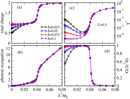
Figure 7: (Color online) Variation with $\lambda^{2}/\omega_{0}$ of (a) the ground-state molecular charge $\langle n_{\mathrm{mol}}\rangle=\langle n_{e}+n_{o}\rangle$, (b) the ground-state phonon occupation $\langle n_{b}\rangle$, (c) the crossover temperature $T^{*}$, and (d) the zero-temperature linear conductance $G$, all calculated for $U^{\prime}=U=0.5$, $\lambda^{\prime}=\lambda$, and the four values of $\delta=\varepsilon_{\beta}=-\varepsilon_{\alpha}$ listed in the legend. In the case $\delta=0.05$, the orbital energy splitting is in resonance with the phonon energy, i.e., $\varepsilon_{\beta}-\varepsilon_{\alpha}=2\delta=\omega_{0}$.

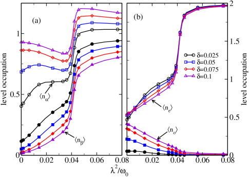
Figure 8: (Color online) Occupation of individual molecular orbitals vs $\lambda^{2}/\omega_{0}$ for $U^{\prime}=U=0.5$, $\lambda^{\prime}=\lambda$, and the four values of $\delta=\varepsilon_{\beta}=-\varepsilon_{\alpha}$ listed in the legend: (a) $\langle n_{\alpha}\rangle$ (open symbols) and $\langle n_{\beta}\rangle$ (filled symbols); (b) $\langle n_{e}\rangle$ (open symbols) and $\langle n_{o}\rangle$ (filled symbols).

IV.2.2 Both orbitals close to the chemical potential

This subsection presents numerical solutions of the full problem under variation of the e-ph coupling. As before, we focus primarily on the reference case $\lambda^{\prime}=\lambda$, $U^{\prime}=U=0.5$.

Figure 7 plots the evolution with $\lambda^{2}/\omega_{0}$ of the same properties as appear in Fig. 5 for four values of $\delta$ chosen so that the two figures differ only as to the energy of the upper molecular orbital: $\varepsilon_{\beta}=4\gg U$ in the earlier figure versus $\varepsilon_{\beta}=\delta\ll U$ here. The results in the two figures are superficially similar, although there are some significant differences as will be explained below.

We begin by considering the behavior for $\lambda=0$. Figure 7(a) shows the zero-temperature molecular charge $\langle n_{\mathrm{mol}}\rangle$, while Fig. 8 displays the corresponding occupancies of individual molecular orbitals: $\langle n_{\alpha}\rangle$ and $\langle n_{\beta}\rangle$ in panel (a), and $\langle n_{e}\rangle$ and $\langle n_{o}\rangle$ in panel (b). For $\delta\ll\Gamma=\pi V^{2}/D\simeq 0.0177$, $\langle n_{\mathrm{mol}}\rangle\simeq\langle n_{e}\rangle\simeq 0.5$, which may be understood as a consequence of the ground state being close to that for $U=V=\infty$ and $\delta=0$: a product of (1) ${\textstyle\frac{1}{2}}\bigl{[}c_{e\uparrow}^{{\dagger}}d_{e\downarrow}^{{\dagger}}-c_{e\downarrow}^{{\dagger}}d_{e\uparrow}^{{\dagger}}-\sqrt{2}c_{e\uparrow}^{{\dagger}}c_{e\downarrow}^{{\dagger}}\bigr{]}|0\rangle$ where $c_{e\sigma}=(2N_{s})^{-1/2}\sum_{\mathbf{k}}c_{e\mathbf{k}\sigma}$ annihilates an electron in the linear combination of left- and right-lead states that tunnels into/out of the molecular orbitals, and (2) other lead degrees of freedom that are decoupled from the molecule. The total charge increases with $\delta$ and approaches $\langle n_{\mathrm{mol}}\rangle=\langle n_{\alpha}\rangle=1$ for $\delta\gg\Gamma$, in which limit the large Coulomb repulsion $U$ leads to local-moment formation in the $\alpha$ orbital, followed at low temperatures by Kondo screening, very much in the same manner as found for $\varepsilon_{\beta}=4$ (Sec. IV.1.3).

Turning on e-ph couplings $\lambda^{\prime}=\lambda$ lowers the energy of the even-parity molecular orbital below that of the odd orbital, and initially drives the system toward $\langle n_{e}\rangle=1$, $\langle n_{o}\rangle=0$, and toward a many-body singlet ground state formed between the leads and a local moment in the even-parity molecular orbital (rather than the local moment in the $\alpha$ orbital that is found for $\varepsilon_{\beta}=4$). The spin-screening scale $T^{*}$ in Fig. 7(c) shows an initial decrease with increasing $\lambda^{2}/\omega_{0}$ that is very strong for the smaller values for $\delta$, where the e-ph coupling drives the system from mixed valence into the Kondo regime. For larger $\delta$, where the system is in the Kondo limit even at $\lambda=0$, there is a much milder reduction of $T^{*}$ caused by the phonon-induced shift of the filled molecular orbital further below the chemical potential.

Upon further increase in the e-ph coupling, $\langle n_{\mathrm{mol}}\rangle$ and $T^{*}$ both show rapid but continuous rises around some value $\lambda=\lambda_{x}$. The crossover value $\lambda_{x}^{2}/\omega_{0}\simeq 0.042$, which is independent of $\delta$ for $\delta\ll U$, coincides closely with its $\delta=0$ value $U/12\simeq 0.0417$ for the isolated molecule, where it describes the crossing of the singly occupied state $|\phi_{1}^{(1)}\rangle$ and the doubly occupied state $|\phi_{1}^{(2)}\rangle$ (see Table 1). For $\Gamma>0$, the crossover of the ground-state molecular charge from 1 to 2 is smeared over the range $|U-12\lambda^{2}/\omega_{0}|\lesssim 2\Gamma$, suggesting a full width for the crossover $\Delta(\lambda^{2}/\omega_{0})\simeq 4\Gamma/12=0.006$, in good agreement with Figs. 7(a) and 8. The values of $\lambda_{x}$ and $\Delta(\lambda^{2}/\omega_{0})$ are smaller than the corresponding values for $\varepsilon_{\beta}=4$ by factors of roughly 3 and 2, respectively, a consequence of the stronger e-ph effects found for small molecular orbital energy separation. Moreover, the absence of any dependence of $\lambda_{x}$ on $\delta$ is to be contrasted with the linear dependence of the crossover e-ph coupling on $\varepsilon_{\alpha}$ in Fig. 5.

In the regime $\lambda\gtrsim\lambda_{x}$, the system minimizes the e-ph energy by adopting orbital occupancies $\langle n_{e}\rangle\simeq 2$, $\langle n_{o}\rangle\simeq 0$ (shown in Fig. 8 to hold for all the $\delta$ values considered). Here, $T^{*}$ approaches the scale $12\lambda^{2}/\omega_{0}-U$ at which occupation of $n_{\mathrm{mol}}=1$ molecular states becomes frozen out. Over the entire range of $\delta$ and $\lambda^{2}/\omega_{0}$ illustrated in Figs. 7 and 8, the ground-state phonon occupation $\langle n_{b}\rangle$ [Fig. 7(b)] closely tracks $\bar{n}_{b}$ and the $T=0$ conductance [Fig. 7(d)] is everywhere well-described by Eq. (55).

We note that the equilibrium properties shown in Figs. 7 and 8 exhibit no special features in the resonant case $\delta=0.05$ in which the molecular orbital spacing $\varepsilon_{\beta}-\varepsilon_{\alpha}$ exactly matches the phonon energy. We expect the resonance condition to play a significant role only in driven setups where a nonequilibrium phonon distribution serves as a net source or sink of energy for the electron subsystem.

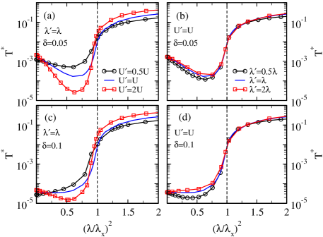
Figure 9: (Color online) Crossover temperature $T^{*}$ vs scaled e-ph coupling $(\lambda/\lambda_{x})^{2}$. The left panels show different ratios $U^{\prime}/U$ for $\lambda^{\prime}=\lambda$ while the right panels show different $\lambda^{\prime}/\lambda$ for $U^{\prime}=U$. The upper panels (a), (b) correspond to an orbital separation $\delta=0.05$, and the lower panels (c), (d) treat $\delta=0.1$. All data are for $U=0.5$. Vertical dashed lines at $\lambda=\lambda_{x}$ [calculated via the condition $E^{(2)}_{\min}(\delta=0)=E^{(1)}_{\min}(\delta=0)$] separate the Kondo regime from the phonon-dominated regime.

The properties presented above are little changed under relaxation of the assumptions $\lambda^{\prime}=\lambda$ and $U^{\prime}=U$. For reasons of space, we show data only for the variation of the crossover temperature $T^{*}$ with e-ph coupling with different fixed values of $U^{\prime}/U$ [Figs. 9(a) and 9(c)] or $\lambda^{\prime}/\lambda$ [Figs. 9(b) and 9(d)]. In each case, $T^{*}$ is plotted against $(\lambda/\lambda_{x})^{2}$, where $\lambda_{x}$ is the value of $\lambda$ that satisfies the condition $E^{(2)}_{\min}(\delta=0)=E^{(1)}_{\min}(\delta=0)$ for crossover from single to double occupation of the isolated molecule. For $U^{\prime}=0.5U$ and $U^{\prime}=2U$, it must be recognized that $J={\textstyle\frac{1}{2}}(U^{\prime}-U)$ is not small, calling into question the validity of the approximation $\hat{n}_{b}=0$ used to derive the energies in Table 1. What is more, the data shown are for nonzero orbital energy splittings $\delta=0.05$ (upper panels) and $\delta=0.1$ (lower panels). Nonetheless, the plots all exhibit good data collapse along the horizontal axis, showing that $\lambda_{x}$ calculated for $\hat{n}_{b}=0$ and $\delta=0$ captures very well the scale characterizing the crossover from the Kondo regime ($\lambda\lesssim\lambda_{x}$) to the phonon-dominated regime ($\lambda\gtrsim\lambda_{x}$).

The data in Fig. 9 show greater spread along the vertical axis, particularly in the Kondo regime under variation of $U^{\prime}/U$. However, we find that in each panel, the value of $T^{*}$ in the phonon-dominated regime can be reproduced with good quantitative accuracy by applying the condition $T^{*}\chi(T*)=0.0701$ to the susceptibility of the isolated molecule, calculated using the eleven states listed in Table 1. This provides further evidence for the adequacy of the approximation $\hat{n}_{b}=0$ employed in the construction of the table. More importantly, Fig. 9 shows that the physics probed in Figs. 7 and 8 for the special case $\lambda^{\prime}=\lambda$ and $U^{\prime}=U$ is broadly representative of the behavior over a wide region of the model’s parameter space.

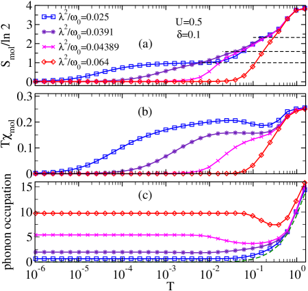
Figure 10: (Color online) Temperature dependence of (a) the molecular entropy, (b) temperature times the molecular susceptibility, $T\chi_{\mathrm{mol}}\equiv|\bm{\mu}_{\mathrm{mol}}|^{2}/3$, where $\bm{\mu}_{\mathrm{mol}}$ is the molecule’s magnetic moment, and (c) the phonon occupation. Data are for $U^{\prime}=U=0.5$, $\delta=0.1$, $\lambda^{\prime}=\lambda$, and the four values of $\lambda^{2}/\omega_{0}$ listed in the legend. In (a), the horizontal dashed lines mark $S_{\mathrm{mol}}=\ln 2$, $\ln 3$, and $\ln 5$. In (c), the dashed line shows the occupation of a free phonon mode of energy $\omega_{0}=0.1$.

To this point, we have concentrated on ground-state ($T=0$) properties and the temperature scale $T^{*}$ characterizing the quenching of the molecular magnetic moment. We now illustrate the full temperature dependence of three thermodynamic properties in situations where the molecular orbitals are arranged symmetrically around the chemical potential. Figure 10 plots the variation with $T$ of the molecular entropy, molecular susceptibility, and phonon occupation for $U^{\prime}=U=0.5$, $\delta=0.1$, $V=0.075$, and four different values of $\lambda^{\prime}=\lambda$. As long as the temperature exceeds all molecular energy scales, the entropy and susceptibility are close to the values $S_{\mathrm{mol}}=\ln 4$ and $T\chi_{\mathrm{mol}}=1/8$ attained when every one of the 16 molecular configurations has equal occupation probability, while the phonon occupation is close to the Bose-Einstein result for a free boson mode of energy $\omega_{0}$ [dashed line in Fig. 10(c)]. Once the temperature drops below $U$, most of the molecular configurations (and all with total charge $n_{\mathrm{mol}}>2$) become frozen out. For $\lambda\ll\lambda_{x}$ (exemplified by $\lambda^{2}/\omega_{0}=0.025$ in Fig. 10), there is a slight shoulder in the entropy around $S_{\mathrm{mol}}=\ln 5$ and a minimum in the square of the local moment around $T\chi_{\mathrm{mol}}=1/5$, the values expected when the empty and singly occupied molecular configurations (the first five states listed in Table 1 are quasidegenerate. At lower temperatures, there is an extended range of local-moment behavior ($S_{\mathrm{mol}}=\ln 2$, $T\chi_{\mathrm{mol}}\simeq 1/4$) associated with single occupancy of the even-parity molecular orbital (states $|\phi^{(1)}_{1}\rangle$ and $|\phi^{(1)}_{2}\rangle$). Eventually, the properties cross over below the temperature scale $T^{*}$ defined above to those of the Kondo singlet state: $S_{\mathrm{mol}}=0$, $T\chi_{\mathrm{mol}}=0$.

For $\lambda$ just below $\lambda_{x}$ ($\lambda^{2}/\omega_{0}=0.0391$ in Fig. 10) there are weak shoulders near $S_{\mathrm{mol}}=\ln 5$ and $T\chi_{\mathrm{mol}}=1/5$, as in the limit of smaller e-ph couplings. In this case, however, these features reflect the near degeneracy of the four $n_{\mathrm{mol}}=1$ configurations and the lowest-energy $n_{\mathrm{mol}}=2$ configuration: $|\phi^{(2)}_{1}\rangle$ in Table 1. At slightly lower temperatures, the states $|\phi^{(1)}_{3}\rangle$ and $|\phi^{(1)}_{4}\rangle$ become depopulated and the properties drop through $S_{\mathrm{mol}}=\ln 3$ and $T\chi_{\mathrm{mol}}=1/6$ before finally falling smoothly to zero. Even though there is no extended regime of local-moment behavior, the asymptotic approach of $S_{\mathrm{mol}}$ and $T\chi_{\mathrm{mol}}$ to their ground state values is essentially identical to that for $\lambda\ll\lambda_{x}$ after rescaling of the temperature by $T^{*}$. As shown in Fig. 11, throughout the regime $\lambda<\lambda_{x}$, $T\chi_{\mathrm{mol}}$ follows the same function of $T/T^{*}$ for $T\lesssim 10T^{*}$. This is just one manifestation of the universality of the Kondo regime, in which $T_{K}\equiv T^{*}$ serves as the sole low-energy scale.

A small increase in $\lambda^{2}/\omega_{0}$ from $0.0391$ to $0.04389$, slightly above $\lambda_{x}^{2}/\omega_{0}=0.0417$, brings about significant changes in the low-temperature properties. While there are still weak features in the entropy at $\ln 5$ and $\ln$3, the final approach to the ground state is more rapid than for $\lambda<\lambda_{x}$, as can be seen from Fig. 11. Note also the upturn in $\langle n_{b}\rangle$ as $T$ falls below about $10T^{*}$—a feature absent for $\lambda<\lambda_{x}$ that signals the integral role played by phonons in quenching the molecular magnetic moment.

Finally, in the limit $\lambda\gg\lambda_{x}$ (exemplified by $\lambda^{2}/\omega_{0}=0.064$ in Fig. 10), $E^{(2)}_{1}$ is by a considerable margin the lowest eigenvalue of $\hat{P}_{0}\hat{H}_{\mathrm{e}}\hat{P}_{0}$, so with decreasing temperature, $S_{\mathrm{mol}}$ and $T\chi_{\mathrm{mol}}$ quickly approach zero with little sign of any intermediate regime. Even though the quenching of the molecular degrees of freedom arises from phonon-induced shifts in the molecular orbitals rather than from a many-body Kondo effect involving strong entanglement with the lead degrees, the $\lambda\to\infty$ ground state is adiabatically connected to that for $\lambda=0$.

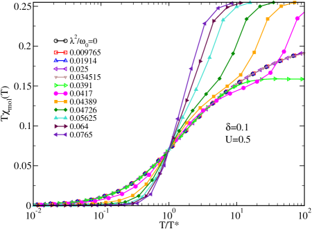
Figure 11: (Color online) Magnetic moment $\mu^{2}=T\chi_{\mathrm{mol}}$ vs scaled temperature $T/T^{*}$ for $U^{\prime}=U=0.5$, $\lambda^{\prime}=\lambda$, $\delta=0.1$, and values of $\lambda^{2}/\omega_{0}$ spanning the crossover from the Kondo regime to the doubly occupied regime. The collapse over the range $T\lesssim 10T^{*}$ of all curves corresponding to $\lambda^{2}/\omega_{0}\leq 0.0391$ demonstrates the universal physics of the Kondo regime. No such universality is present in the boson-dominated limit.

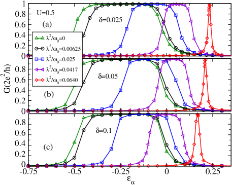
Figure 12: (Color online) Zero-temperature conductance $G$ as a function of $\varepsilon_{\alpha}=-\delta-V_{g}$ (where $V_{g}$ is an applied gate voltage) for the five values of $\lambda^{2}/\omega_{0}$ listed in the legend and (a) $\delta=0.025$, (b) $\delta=0.05$, and (c) $\delta=0.1$. The other parameters are $U^{\prime}=U=0.5$ and $\lambda^{\prime}=\lambda$.

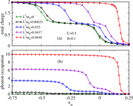
Figure 13: (Color online) (a) Ground-state molecular charge and (b) ground-state phonon occupation as functions of $\varepsilon_{\alpha}=-\delta-V_{g}$ (where $V_{g}$ is an applied gate voltage) for $\delta=0.1$ and the values of $\lambda^{2}/\omega_{0}$ listed in the legend. The other parameters are $U^{\prime}=U=0.5$ and $\lambda^{\prime}=\lambda$.

IV.2.3 Effect of a uniform shift in the orbital energies

We finish by considering the effect of shifting the two molecular orbitals at a fixed, small energy separation $\varepsilon_{\beta}-\varepsilon_{\alpha}=2\delta$ through the application of a gate voltage $V_{g}$ that causes $\varepsilon_{i}$ in Eq. (2) to be replaced by $\varepsilon_{i}-eV_{g}$, and $\tilde{\varepsilon}_{p}$ in Eq. (II.2) to be replaced by $\tilde{\varepsilon}_{p}-eV_{g}$. Figure 12 plots the gate-voltage dependence of the linear conductance for $U^{\prime}=U=0.5$, five values of $\lambda^{\prime}=\lambda$, and for $\delta=0.025$ [panel (a)], $\delta=0.05$ (b), and $\delta=0.1$ (c). Figure 13 shows the corresponding evolution of the total molecular charge and the phonon occupation for the case $\delta=0.1$. In both figures, the quantity plotted along the horizontal axis is $\varepsilon_{\alpha}=-\delta-eV_{g}$, which allows direct comparison with the results shown in in Figs. 2(c), 2(f), and 3(c) for the regime where the $\beta$ molecular orbital lies far above the chemical potential.

Just as in the other situations considered above, the zero-temperature conductance obeys the Fermi-liquid relation Eq. (55). A plateau at $G\simeq G_{0}$ spans the range of gate voltages within which the total molecular occupancy is $\langle n_{\mathrm{mol}}\rangle\simeq 1$ [e.g., compare Figs. 12(c) and 13(a)], while the conductance approaches zero for larger $V_{g}$, where the molecular charge vanishes, and for smaller $V_{g}$, where $\langle n_{\mathrm{mol}}\rangle\simeq 2$.

Once again, we begin by considering the limit $\lambda=0$ of zero e-ph coupling. For $\delta=0.025\ll\Gamma=0.0177$, the rises between zero and peak conductance are somewhat broader (along the $\varepsilon_{\alpha}$ axis) than their counterparts in cases where the $\beta$ molecular orbital lies far above the chemical potential [compare with Fig. 3(c)]. This broadening can be understood as a consequence of the step in $\langle n_{\mathrm{mol}}\rangle$ being split into changes in $\langle n_{\alpha}\rangle$ and in $\langle n_{\beta}\rangle$. When $\delta\gg\Gamma$, the $\beta$ molecular orbital is essentially depopulated [as can be seen for the $V_{g}=0$ in Fig. 8(a)] and the conductance steps narrow to a width similar to that for $\varepsilon_{\beta}=4$.

Increase of the e-ph coupling from zero results in shifts of the occupancy and conductance steps to progressively higher values of $\varepsilon_{\alpha}$ (or to lower values of $V_{g}$) that can be attributed to the phonon-induce renormalization of the orbital energies and of the Coulomb interactions. For $\delta=0.025$, the width of the $\langle n_{\mathrm{mol}}\rangle\simeq 1$, $G\simeq G_{0}$ plateau is close to the value $\tilde{\tilde{U}}$ defined in Eq. 60, which approaches $U-8\lambda^{2}/\omega_{0}$ in the limit $\delta\lesssim\lambda^{2}/\omega_{0}$ satisfied by the $\delta=0.025$ curves in Eq. 12(a). Even for the $\delta=0.1$ curves shown in Fig. 12(b), the plateau width is at least $U-8\lambda^{2}/\omega_{0}$, considerably larger than than its value $\tilde{U}=U-2\lambda^{2}/\omega_{0}$ when the orbital $\beta$ lies far above the chemical potential. The occupancy and conductance plateau might be expected to disappear once $\tilde{\tilde{U}}$ becomes negative around $\lambda^{2}/\omega_{0}\simeq U/8=0.0625$. Indeed, the data for $\lambda^{2}/\omega_{0}=0.064$ in Fig. 12 show a narrow conductance peak that can be associated with the rapid decrease of $\langle n_{\mathrm{mol}}\rangle$ directly from 2 to 0 without any significant range of single occupancy [illustrated for $\delta=0.1$ in Fig. 13(b)].

V Summary

We have studied the low-temperature properties of a single-molecule junction formed by a two-orbital molecule connecting metallic leads. The model Hamiltonian incorporates intraorbital and interorbital Coulomb repulsion, a Holstein coupling of the molecular charge to the displacement of a local phonon mode, and also phonon-mediated interorbital tunneling. We have investigated the low-temperature regime of the system using the numerical renormalization group to provide a nonperturbative treatment of the competing strong interactions. Insight into the numerical results has been obtained by considering the phonon-renormalization of model parameters identified through canonical transformation of the starting Hamiltonian.

We have focused on two quite different regions of the model’s parameter space: (1) In situations where one of the two molecular orbitals lies close to the chemical potential while the other has a much higher energy, the thermodynamic properties and linear conductance are very similar to those predicted previously for a single-orbital molecule, showing phonon-induced shifts in the active molecular orbital and a reduction in the effective Coulomb repulsion between electrons on the molecule. In this region, interorbital e-ph coupling can be treated as a weak perturbation. (2) In the region in which the two orbitals both lie close to the chemical potential, where all the interactions must be treated on an equal footing, the phonon-induced renormalization of the Coulomb interactions is stronger than in the case of one active molecular orbital, enhancing the likelihood of attaining in experiments the interesting regime of small or even attractive on-site Coulomb interactions.

In both regions (1) and (2), electron-phonon interactions favor double occupancy of the molecule and are detrimental to formation of a molecular local moment and to the low-temperature Kondo screening of that moment by electrons in the leads. With increasing electron-phonon coupling, the Kondo effect is progressively destroyed and a phonon-dominated nonmagnetic ground state emerges in its place. In all the cases presented here, this evolution produces a smooth crossover in the ground-state properties. Special situations that result in first-order quantum phase transitions between Kondo and non-Kondo ground states will be described in a subsequent publication. We have left for future study cases involving two degenerate (or nearly degenerate) molecular orbitals lying below the chemical potential of the leads. In such cases, e-e interactions favor the presence of an unpaired electron in each orbital, and electron-phonon interactions may be expected to significantly affect the competition between total-spin-singlet and triplet ground states.Hofstetter:2002 ; Gordon:2003 ; Nature:453-366