Rounding of a first-order quantum phase transition to a strong-coupling critical point

Abstract

We investigate the effects of quenched disorder on first-order quantum phase transitions on the example of the $N$-color quantum Ashkin-Teller model. By means of a strong-disorder renormalization group, we demonstrate that quenched disorder rounds the first-order quantum phase transition to a continuous one for both weak and strong coupling between the colors. In the strong coupling case, we find a distinct type of infinite-randomness critical point characterized by additional internal degrees of freedom. We investigate its critical properties in detail and find stronger thermodynamic singularities than in the random transverse field Ising chain. We also discuss the implications for higher spatial dimensions as well as unusual aspects of our renormalization-group scheme.

I Introduction

The effects of disorder on quantum phase transitions have gained increasing attention recently, in particular since experiments have discovered several of the exotic phenomena predicted by theory (see, e.g., Refs. Vojta, 2006, 2010). Most of the existing work has focused on continuous transitions while first-order quantum phase transitions have received less attention.

In contrast, the influence of randomness on pure systems undergoing a classical first-order transition has been comprehensively studied. Using a beautiful heuristic argument, Imry and Wortis Imry and Wortis (1979) reasoned that quenched disorder should round classical first-order phase transitions in sufficiently low dimension and thus produce new continuous phase transitions. This analysis was extended by Hui and Berker.Hui and Berker (1989) Aizenman and Wehr Aizenman and Wehr (1989) rigorously proved that first-order phase transitions cannot exist in disordered systems in dimensions $d\leq 2$. If the randomness breaks a continuous symmetry, the marginal dimension is $d=4$.

The question of whether or not disorder can round a first-order quantum phase transition (QPT) to a continuous one was asked by Senthil and Majumdar,Senthil and Majumdar (1996) and, more recently, by Goswami et al.Goswami et al. (2008) Using a strong-disorder renormalization group (SDRG) technique, they found that the transitions in the random quantum Potts and clock chains Senthil and Majumdar (1996) were governed by the well-known infinite-randomness critical point (IRCP) of the random transverse-field Ising chain.Fisher (1992, 1995) The same holds for the $N$-color quantum Ashkin-Teller (AT) model in the weak-coupling (weak interaction between the colors) regime.Goswami et al. (2008) This implies that disorder can indeed round first-order quantum phase transitions.

In the strong-coupling regime of the AT model, on the other hand, the renormalization-group (RG) analysis of the authors of Ref. Goswami et al., 2008 breaks down. Goswami et al. speculated that this implies persistence of the first-order QPT in the presence of disorder, requiring important modifications of the Aizenman-Wehr theorem. However, shortly after, Greenblatt et al. Greenblatt et al. (2009, 2012) proved rigorously that the Aizenman-Wehr theorem also holds for quantum systems at zero temperature.

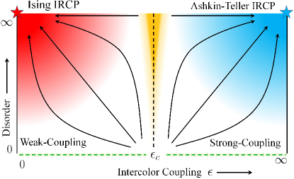
Figure 1: (Color online) Schematic of the renormalization-group flow diagram in the disorder—coupling strength parameter space. For $\epsilon<\epsilon_{c}$ (left arrows), the critical flow approaches the usual Ising infinite-randomness critical point of Ref. Fisher, 1995. For $\epsilon>\epsilon_{c}$ (right arrows), we find a distinct infinite-randomness critical point with even stronger thermodynamic singularities.

In this paper, we resolve the apparent contradiction between these results. We show that quenched disorder rounds the first-order QPT of the AT model in the strong-coupling regime as well as in the weak-coupling regime. Moreover, we unveil a distinct type of infinite-randomness critical point governing the transition in the strong-coupling regime. It is characterized by additional internal degrees of freedom which appear because a higher symmetry is dynamically generated at criticality. As a consequence, the critical point displays even stronger thermodynamic singularities than the transverse-field Ising IRCP. To obtain these results, we have developed an implementation of the SDRG method that works for both weak and strong coupling. In particular, this method can deal with the diverging intercolor interactions as well as the associated additional degeneracies. A schematic of the resulting RG flow in the critical plane is shown in Fig. 1.

Our paper is organized as follows: In Sec. II, we define the model and discuss a few of its basic properties. Section III is devoted to our strong-disorder renormalization group scheme. The resulting phase diagram and observables are discussed in Sec. IV. We conclude in Sec. V.

II Quantum Ashkin-Teller model

The Hamiltonian of the one-dimensional $N$-color quantum AT model Grest and Widom (1981); Fradkin (1984); Shankar (1985) is given by

$$\begin{gathered}H=-\sum_{\alpha=1}^{N}\sum_{i=1}^{L}{\left(J_{i}\sigma_{\alpha,i}^{z}\sigma_{\alpha,i+1}^{z}+h_{i}\sigma_{\alpha,i}^{x}\right)}\\ -\sum_{\alpha<\beta}^{N}\sum_{i=1}^{L}{\left(\epsilon_{J,i}J_{i}\sigma_{\alpha,i}^{z}\sigma_{\alpha,i+1}^{z}\sigma_{\beta,i}^{z}\sigma_{\beta,i+1}^{z}+\epsilon_{h,i}h_{i}\sigma_{\alpha,i}^{x}\sigma_{\beta,i}^{x}\right)}.\end{gathered}$$ (1)

Here, $i$ indexes the lattice sites, $\alpha$ and $\beta$ index colors, and $\sigma^{x}$ and $\sigma^{z}$ are the usual Pauli matrices. The interactions $J_{i}$ and transverse fields $h_{i}$ are independent random variables taken from distributions restricted to positive values, while $\epsilon_{h,i}$ and $\epsilon_{J,i}$ (also restricted to be positive) parametrize the strength of the coupling between the colors. Various versions of the AT model have been used to describe the layers of atoms absorbed on surfaces, organic magnets, current loops in high-$T_{c}$ superconductors as well as the elastic response of DNA molecules. Note the invariance of the Hamiltonian under the following duality transformation: $\sigma_{\alpha,i}^{z}\sigma_{\alpha,i+1}^{z}\to\tau_{\alpha,i}^{x}$, $\sigma_{\alpha,i}^{x}\to\tau_{\alpha,i}^{z}\tau_{\alpha,i+1}^{z}$, $J_{i}\rightleftarrows h_{i}$, and $\epsilon_{J,i}\rightleftarrows\epsilon_{h,i}$, where $\tau^{x}$ and $\tau^{z}$ are the dual Pauli operators. The bulk phases of the AT model (1) are easily understood. If the typical interaction $J_{typ}$ is larger than the typical field $h_{typ}$, the system is in the ordered (Baxter) phase in which each color orders ferromagnetically. When $h_{typ}\gg J_{typ}$, the model is in the paramagnetic phase. If there is a direct transition between these two phases, duality requires that it occurs at $J_{typ}=h_{typ}$. In the clean version of our system with $N\geq 3$, the QPT between the paramagnetic and ordered (Baxter) phases is of first-order type.Grest and Widom (1981); Fradkin (1984); Shankar (1985); Ceccatto (1991)

III Strong-Disorder Renormalization Group

To tackle the Hamiltonian (1), we now develop a SDRG method. In the weak-coupling regime ($\epsilon_{h},\epsilon_{J}\ll\epsilon_{c}$, where $\epsilon_{c}$ is some $N$-dependent threshold), our method agrees with that of Goswami et al.Goswami et al. (2008) Here, we focus on the strong coupling regime $\epsilon_{h},\epsilon_{J}\gg\epsilon_{c}$ where the method of the authors of Ref. Goswami et al., 2008 breaks down.

The basic idea of the SDRG method consists in identifying the largest local energy scale and perturbatively integrating out the corresponding high-energy degree of freedom. As we are in the strong-coupling regime, this largest local energy is either a four-spin interaction (“AT interaction”) $k_{i}=\epsilon_{J,i}J_{i}$ or a two-color field-like term (“AT field”) $g_{i}=\epsilon_{h,i}h_{i}$. We thus define our high-energy cutoff $\Omega=\max\{k_{i},g_{i}\}$.

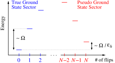
Figure 2: (Color online) Spectrum of the unperturbed Hamiltonian (2) as function of the number of colors flipped with respect to the ground state $\left|\to,\to,\cdots,\to\right\rangle$. As long as $T\lesssim\Omega/\epsilon_{h}$, the pseudo ground state $|\phi_{0}^{\prime}\rangle=\left|\leftarrow,\leftarrow,\cdots,\leftarrow\right\rangle$ can be neglected when computing observables (stage 1 of the RG). When $T\gtrsim\Omega/\epsilon_{h}$, $|\phi_{0}\rangle$ and $|\phi_{0}^{\prime}\rangle$ become effectively degenerate implying that both states need to be taken into account (stage 2 of the RG).

We now derive the decimation procedure. If the largest local energy is an AT field located, say, at site $2$, the unperturbed Hamiltonian for the decimation of this site reads

$$H_{0}=-\frac{g_{2}}{\epsilon_{h,2}}\sum_{\alpha=1}^{N}{\sigma_{\alpha,2}^{x}}-g_{2}\sum_{\alpha<\beta}{\sigma_{\alpha,2}^{x}\sigma_{\beta,2}^{x}}.$$ (2)

The ground state (GS) of $H_{0}$ is $\left|\phi_{0}\right\rangle=\left|\to,\to,\cdots,\to\right\rangle$, with energy $E_{0}=-Ng_{2}/\epsilon_{h,2}-N(N-1)g_{2}/2$, where each arrow represents a different color. Flipping $n$ colors leads to $\binom{N}{n}$ degenerate excited states with energy $E_{n}=E_{0}+2ng_{2}/\epsilon_{h,2}+2n(N-n)g_{2}$. In the strong-coupling regime, $\epsilon_{h}\gg 1$, the state $\left|\phi_{0}^{\prime}\right\rangle=\left|\leftarrow,\leftarrow,\cdots,\leftarrow\right\rangle$ plays a special role. Its energy $E_{0}^{\prime}=Ng_{2}/\epsilon_{h,2}-N(N-1)g_{2}/2$ differs from that of the true ground state only by the subleading Ising term $E_{0}^{\prime}-E_{0}=2Ng_{2}/\epsilon_{h,2}$ (see Fig. 2). It can thus be considered a “pseudo ground state” which may be important for a correct description of the low-energy physics. The true and pseudo ground states each have their own sets of low-energy excitations which we call the ground-state and pseudo-ground-state sectors of low energy states.

The couplings of site 2 to its neighbors,

$$\begin{gathered}V=-\frac{k_{1}}{\epsilon_{J,1}}\sum_{\alpha=1}^{N}{\sigma_{\alpha,1}^{z}\sigma_{\alpha,2}^{z}}-k_{1}\sum_{\alpha<\beta}{\sigma_{\alpha,1}^{z}\sigma_{\alpha,2}^{z}\sigma_{\beta,1}^{z}\sigma_{\beta,2}^{z}}\\ -\frac{k_{2}}{\epsilon_{J,2}}\sum_{\alpha=1}^{N}{\sigma_{\alpha,2}^{z}\sigma_{\alpha,3}^{z}}-k_{2}\sum_{\alpha<\beta}{\sigma_{\alpha,2}^{z}\sigma_{\alpha,3}^{z}\sigma_{\beta,2}^{z}\sigma_{\beta,3}^{z}},\end{gathered}$$ (3)

is the perturbation part of the Hamiltonian. We now decimate site 2 in the second-order perturbation theory, keeping both the true ground state and the pseudo ground state. It is important to note that second-order perturbation theory does not mix states from the two sectors as long as $N>4$. (The sectors are coupled in a higher order of perturbation theory, but these terms are irrelevant at our IRCP). After decimating site 2, the effective interaction Hamiltonian of the neighboring sites reads (in the large-$\epsilon_{J}$ limit)

$$\tilde{H}_{eff}=-\frac{\tilde{k}}{\tilde{\epsilon}_{J}}\sum_{\alpha=1}^{N}{\sigma_{\alpha,1}^{z}\sigma_{\alpha,3}^{z}}-\tilde{k}\sum_{\alpha<\beta}{\sigma_{\alpha,1}^{z}\sigma_{\alpha,3}^{z}\sigma_{\beta,1}^{z}\sigma_{\beta,3}^{z}}-\tilde{\omega}\tilde{\zeta},$$ (4)

with

$$\tilde{k}=\frac{k_{1}k_{2}}{2(N-2)g_{2}},~{}~{}~{}\tilde{\epsilon}_{J}=\frac{\epsilon_{J,1}\epsilon_{J,2}}{2}\frac{N-1}{N-2},~{}~{}~{}\tilde{\omega}=Ng_{2}/\epsilon_{h,2}.$$ (5)

Here, $\tilde{\zeta}=\pm 1$ is a new Ising degree of freedom which represents the energy splitting between the true and the pseudo ground states. In the large-$\epsilon_{J}$ regime, it is only very weakly coupled to the rest of the chain and can be considered free. In Fig. 3(a), we sketch this decimation procedure.

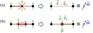
Figure 3: (Color online) a) Decimating a site results in a renormalized bond (characterized by $\tilde{k}$ and $\tilde{\epsilon}_{J}$) between its neighbors, and it introduces an extra binary “sector” degree of freedom represented as an Ising spin $\tilde{\zeta}=\pm 1$ in an external field $\tilde{\omega}$ [see Eq. (7)]. b) Decimating a bond results in a renormalized site characterized by $\tilde{g}$, $\tilde{\epsilon}_{h}$ and another sector degree of freedom.

The decimation of a bond can be treated in the same way. If an AT four-spin interaction, say $k_{2}$, is the largest local energy, the unperturbed Hamiltonian reads

$$H_{0}=-\frac{k_{2}}{\epsilon_{J}}\sum_{\alpha=1}^{N}{\sigma_{\alpha,2}^{z}\sigma_{\alpha,3}^{z}}-k_{2}\sum_{\alpha<\beta}^{N}{\sigma_{\alpha,2}^{z}\sigma_{\alpha,3}^{z}\sigma_{\beta,2}^{z}\sigma_{\beta,3}^{z}}.$$ (6)

Its GS is obtained by any sequence of parallel nearest-neighbors pairs (e.g. $|\phi_{0}\rangle=|\uparrow\uparrow,\uparrow\uparrow,\downarrow\downarrow,\downarrow\downarrow,\uparrow\uparrow,\downarrow\downarrow,\cdots,\uparrow\uparrow\rangle$) with energy $E_{0}=-Nk_{2}/\epsilon_{J,2}-N(N-1)k_{2}/2$. As above, in the strong-coupling limit $\epsilon_{J,2}\gg 1$, $H_{0}$ has a pseudo-GS consisting of a sequence of anti-parallel nearest-neighbors pairs (e.g. $|\phi_{0}^{\prime}\rangle=|\uparrow\downarrow,\uparrow\downarrow,\downarrow\uparrow,\downarrow\uparrow,\uparrow\downarrow,\downarrow\uparrow,\cdots,\uparrow\downarrow\rangle$) with energy $E_{0}^{\prime}=Nk_{2}/\epsilon_{J}-N(N-1)k_{2}/2$.

When integrating out the bond, the two-site cluster gets replaced by a single site which contains one additional internal binary degree of freedom, namely, whether the cluster is in the GS sector or in the pseudo-GS sector. Its effective Hamiltonian reads

$$\tilde{H}_{eff}=-\frac{\tilde{g}}{\tilde{\epsilon}_{h}}\sum_{\alpha=1}^{N}{\sigma_{\alpha,2}^{x}}-\tilde{g}\sum_{\alpha<\beta}{\tilde{\sigma}_{\alpha,2}^{x}\tilde{\sigma}_{\beta,2}^{x}}-\tilde{\omega}\tilde{\zeta}$$ (7)

with

$$\tilde{g}=\frac{g_{2}g_{3}}{2k_{2}[N-2]},~{}~{}~{}\tilde{\epsilon}_{h}=\frac{\epsilon_{h,2}\epsilon_{h,3}}{2}\frac{N-1}{N-2},~{}~{}~{}\tilde{\omega}=Nk_{2}/\epsilon_{J,2}.$$ (8)

Here, $\tilde{\zeta}$ distinguishes the two sectors as before. The duality of the Hamiltonian can be seen by comparing Eqs. (5) and (8) after exchanging the roles of $k$ and $g$ as well as $\epsilon_{h}$ and $\epsilon_{J}$.

Note that the magnetic moment $\tilde{\mu}$ of the new effective site depends on the internal degree of freedom $\tilde{\zeta}$ [see Fig. 3(b)] because neighboring spins are parallel in the GS sector but antiparallel in the pseudo-GS sector. We will come back to this point when discussing observables.

The SDRG proceeds by iterating these decimations. In this process, the coupling strengths $\epsilon_{J}$, $\epsilon_{h}$ flow to infinity if their initial values are greater than some $\epsilon_{c}(N)$. This means that the Ising terms $J_{i},h_{i}$ become less and less important with decreasing energy scale $\Omega$. The large-$\epsilon$ approximation thus becomes asymptotically exact. The remaining energies are the AT four-spin interactions $k_{i}$ and the AT fields $g_{i}$. Their recursions relations have the same multiplicative structure as the recursions of Fisher’s solution Fisher (1995) of the random transverse-field Ising model. The flow of the distributions $P(k_{i})$, $R(g_{i})$ and their fixed points are thus identical to those of Fisher’s solution, see Fig. 1. We conclude that the distributions of $k$, $g$ have an infinite-randomness critical fixed point featuring exponential instead of power-law scaling. Fisher (1992, 1995); Rieger and Young (1996) As the Ising coupling $J_{i},h_{i}$ have vanished, this critical fixed point has the symmetry of the AT interaction and field terms which is higher than that of the full Hamiltonian.

IV Phase Diagram and Observables

The zero-temperature phase diagram of our system is determined by the low-energy limit of the SDRG flow. There are three classes of fixed points parameterized by the distance from criticality $r=\ln(g_{typ}/k_{typ})=\langle\ln g\rangle-\langle\ln k\rangle$ (where $\langle\cdots\rangle$ denotes the disorder average): The critical fixed point at $r=0$, and two lines of fixed points for the ordered ($r<0$) and for the disordered ($r>0$) Griffiths phases. This implies that there is a direct continuous phase transition between the ordered (Baxter) and disordered phases. We found no evidence for additional phases or phase transitions. In agreement with the Aizenman-Wehr theorem,Greenblatt et al. (2009) we thus conclude that disorder turns the clean first-order QPT into a continuous QPT in both strong-coupling and weak-coupling regimes.

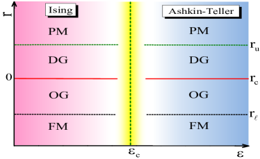
Figure 4: (Color online) Phase diagram of the $N$-color quantum Ashkin-Teller model as function of $r=\ln(h_{typ}/J_{typ})$ and the intercolor coupling $\epsilon$ at fixed disorder strength. The critical line is located at $r=r_{c}=0$ ($J_{typ}=h_{typ}$) as expected from the duality transformation. PM and FM denote the conventional paramagnetic and ferromagnetic (Baxter) phases. OG and DG denote the ordered and disordered Griffiths phases.

We now turn to the behavior of observables at low temperatures. Let us fix the intercolor coupling parameter at some $\epsilon>\epsilon_{c}$ and tune the transition by the ratio $h_{typ}/J_{typ}=g_{typ}/k_{typ}$ (see Fig. 4). The basic idea is as follows.Bhatt and Lee (1982) We decimate the system until the cutoff energy scale $\Omega$ reaches the temperature $T$. For low enough $T$, the distributions of all energy scales in the renormalized system become very broad, and thus, the remaining degrees of freedom can be considered as free. Applying this procedure, we have to distinguish two stages depending on the importance of the pseudo ground state. (1) Both AT and Ising couplings are above the temperature. (In this stage, we decimate sites and bonds whose internal sector degrees of freedom are frozen in the true ground state, $\tilde{\zeta}=1$.) (2) The temperature is below the AT couplings but above the Ising couplings. (Here we still decimate sites and bonds, but their internal degrees of freedom are free, i.e., they can be in either of the two sectors, $\tilde{\zeta}=\pm 1$.)

Let us illuminate this RG scheme on the example of the entropy. When the RG flow stops at $\Omega=T$, all spins are completely free. A surviving cluster has $2^{N}$ available states (two per independent color) giving an entropy contribution of $N\ln 2$, i.e., $S_{\rm chain}=n_{T}N\ln 2$, where $n_{\Omega}$ is the density of surviving clusters at energy scale $\Omega$ (Ref. Fisher (1995)). Moreover, during stage 2 of the flow, residual entropy was accumulated in the internal degrees of freedom, each of them contributing $\ln 2$ to the entropy. Noticing that each stage-2 RG decimation generates one extra degree of freedom, and that stage 2 starts when $\Omega/\epsilon_{J,h}=T$, ($\epsilon_{x}$ is the typical value of $\epsilon_{x,i}$ at energy scale $\Omega$), the extra contribution to the entropy is $S_{\rm extra}=[w_{J}(n_{\epsilon_{J}T}-n_{T})+w_{h}(n_{\epsilon_{h}T}-n_{T})]\ln 2$, with $w_{J}=1-w_{h}$ being the fraction of coupling decimations in the entire stage 2 of the RG flow. To compute $S_{\rm extra}$ we need to know how $\epsilon_{J}$ and $\epsilon_{h}$ depend on $\Omega$. From the recursions (8) and (5), it is clear that $\ln\epsilon_{h}$ (and $\ln\epsilon_{J}$) scale like the number of sites (bonds) in a renormalized cluster (larger bond).

At criticality, $w_{J}=w_{h}=1/2$, $n_{\Omega}\sim[\ln(\Omega_{I}/\Omega)]^{-1/\psi}$, with $\psi=1/2$ being the tunneling exponent, and $\ln\epsilon_{h}=\ln\epsilon_{J}\sim[\ln(\Omega_{I}/\Omega)]^{\phi}$, with $\phi=\frac{1}{2}(1+\sqrt{5})$ (Refs. Fisher (1995) and Vojta et al. (2009)). Thus, summing the two contributions we find that

$$S=C_{1}\left[\ln{\left(\frac{\Omega_{I}}{T}\right)}\right]^{-\frac{1}{\psi\phi}}\ln 2+C_{2}\left[\ln{\left(\frac{\Omega_{I}}{T}\right)}\right]^{-\frac{1}{\psi}}N\ln 2,$$ (9)

where $C_{1}$ and $C_{2}$ are nonuniversal constants, and $\Omega_{I}$ is the bare energy cutoff. As $\phi>1$, the low-$T$ entropy becomes dominated by the extra degrees of freedom $S\to S_{\rm extra}\sim[\ln(\Omega_{I}/T)]^{-1/(\phi\psi)}$.

In the ordered Griffiths phase ($r<0$), $w_{J}\to 1$ and $\ln\epsilon_{J}=Az^{\nu\psi(\phi-1)}\ln(\Omega_{I}/\Omega)$, with $A$ being a nonuniversal constant of order unity, $\nu=2$ the correlation length exponent, and $z=1/(2|r|)$ the dynamical exponent. As $n_{\Omega}\sim|r|^{\nu}(\Omega/\Omega_{I})^{1/z}$, we find that

$$S_{\rm extra}\sim|r|^{\nu}(T/\Omega_{I})^{1/(z+Az^{\phi})}\ln 2,$$ (10)

which dominates over the chain contribution proportional to $T^{1/z}N\ln 2$. As expected from duality, the same result holds for the disordered phase ($r>0$).

To discuss the magnetic susceptibility, we need to find the effective magnetic moment $\mu_{\rm eff}$ of a cluster surviving at the RG energy scale $\Omega=T$. If all internal degrees of freedom were in their ground state, $\mu_{\rm eff}$ would be given by the number of sites in the cluster. However, analogously to the entropy, $\mu_{\rm eff}$ is modified because of the stage 2 of the RG flow. In this stage, the internal degrees of freedom are free, meaning not all spins in a surviving cluster are parallel, reducing the effective moment. A detailed analysis based on the central limit theorem Hrahsheh et al. gives $\mu_{\rm eff}\sim[\ln(\Omega_{I}/T)]^{\phi/2+1/2}$ at criticality and $\mu_{\rm eff}\sim r^{\nu\psi(1-\phi)}[\ln(\Omega_{I}/T)]^{1/2}$ in the disordered Griffiths phase, as well as $\mu_{\rm eff}\sim r^{-\phi/2}T^{-1/(2z)}$ in the ordered Griffiths phase.

The magnetic susceptibility $\chi(T)$ can now be computed. All eliminated clusters had AT fields greater than the temperature, and thus do not contribute to $\chi$ since they are fully polarized in the $x$-direction, whereas the surviving clusters are effectively free and contribute with a Curie term: $\chi\sim\mu_{\rm eff}^{2}n_{T}/T$. We find that

$$\chi\sim[\ln(\Omega_{I}/T)]^{\phi+1-1/\psi}/T$$ (11)

in the critical region, while it becomes

$$\chi\sim r^{\nu+2\nu\psi(1-\phi)}T^{1/z-1}\ln(\Omega_{I}/T)$$ (12)

in the disordered Griffiths phase, and take a Curie form $\chi\sim|r|^{\nu-\phi}T^{-1}$ in the ordered Griffiths phase.

V Conclusion

In summary, we have solved the random quantum Ashkin-Teller model by means of a strong-disorder renormalization-group method that works not just for weak-coupling but also in the strong-coupling regime and yields asymptotically exact results. In the concluding paragraphs, we put our results into broader perspective.

First, we have demonstrated that random disorder turns the first-order QPT between the paramagnetic and Baxter phases into a continuous one not just in the weak-coupling regime but also in the strong-coupling regime. This resolves the seeming contradiction between the quantum Aizenman-Wehr theorem Greenblatt et al. (2009, 2012) and the conclusion that the first-order transition may persist for sufficiently large coupling strength.Goswami et al. (2008)

The resulting continuous transition is controlled by two different IRCPs in the weak and strong coupling regimes. For weak coupling, the critical point is in the universality class of the random transverse-field Ising chain. Fisher (1995) For strong coupling, we find a distinct type of IRCP which features a higher symmetry than the underlying Hamiltonian. The associated internal degrees of freedom lead to even stronger thermodynamic singularities both at criticality and in the Griffiths phases.

Our results apply to $N>4$ colors where the true and pseudo ground-state sectors are not coupled. As a result, the Ising terms in the Hamiltonian are irrelevant perturbations (in the renormalization group sense) at our IRCP. The case $N\leq 4$ is special because the two sectors get coupled and thus requires a separate investigation. Interestingly, novel behavior has been recently verified for the classical transition in the two-dimensional AT model Bellafard et al. (2012) for $N=3$.

Our explicit calculations were for one space dimension. However, we believe that many aspects of our results carry over to higher dimensions. In particular, the SDRG recursion relations take the same form in all dimensions (as they are purely local). This implies that the RG flow for large inter-color coupling $\epsilon$ will be toward $\epsilon\to\infty$ as in one dimension. Moreover, the flows of the AT energies $g$ and $k$ (although not exactly solvable in $d>1$) are identical to the flows of the random transverse-field Ising model in the same dimension. In two and three dimensions, these flows have been studied numerically,Motrunich et al. (2000); Iglói and Monthus (2005); Kovács and Iglói (2011) yielding IRCPs as in one dimension. We thus conclude that the strong-coupling regime of the random quantum AT model will be controlled by an Ashkin-Teller IRCP not just in one dimension but also in two and three dimensions.

We note that our method is also interesting from a general renormalization-group point of view. After a decimation, the resulting system cannot be represented solely in terms of a renormalized quantum AT Hamiltonian because the internal degree of freedom needs to be taken into account. Normally, the appearance of new variables dooms an RG scheme. Here, however, the new variables, despite their influence on observables, are inert in the sense that they do not influence the RG flow of the other terms in the Hamiltonian, which makes the problem tractable. We expect that this insight may be applicable to renormalization-group schemes in other fields.

The strong-disorder RG approach to the random quantum AT model gives asymptotically exact results for both sufficiently weak and sufficiently strong coupling ($\epsilon\ll 1$, $\epsilon\gg 1$), see Fig. 1. The behavior for moderate $\epsilon$ is not exactly solved. In the simplest scenario, the weak-coupling and strong-coupling IRCPs are separated by a unique multicritical point at some intermediate coupling, however, more complicated scenarios cannot be excluded. The resolution of this question will likely come from numerical implementations of the SDRG and /or (quantum) Monte Carlo simulations.

This work has been supported in part by the NSF under Grants No. DMR-0906566 and DMR-1205803, by FAPESP under Grant No. 2010/ 03749-4, and by CNPq under Grants No. 590093/2011-8 and No. 302301/2009-7.

References

- Vojta (2006) T. Vojta, J. Phys. A 39, R143 (2006).
- Vojta (2010) T. Vojta, J. Low Temp. Phys 161, 299 (2010).
- Imry and Wortis (1979) Y. Imry and M. Wortis, Phys. Rev. B 19, 3580 (1979).
- Hui and Berker (1989) K. Hui and A. N. Berker, Phys. Rev. Lett. 62, 2507 (1989).
- Aizenman and Wehr (1989) M. Aizenman and J. Wehr, Phys. Rev. Lett. 62, 2503 (1989).
- Senthil and Majumdar (1996) T. Senthil and S. N. Majumdar, Phys. Rev. Lett. 76, 3001 (1996).
- Goswami et al. (2008) P. Goswami, D. Schwab, and S. Chakravarty, Phys. Rev. Lett. 100, 015703 (2008).
- Fisher (1992) D. S. Fisher, Phys. Rev. Lett. 69, 534 (1992).
- Fisher (1995) D. S. Fisher, Phys. Rev. B 51, 6411 (1995).
- Greenblatt et al. (2009) R. L. Greenblatt, M. Aizenman, and J. L. Lebowitz, Phys. Rev. Lett. 103, 197201 (2009).
- Greenblatt et al. (2012) R. Greenblatt, M. Aizenman, and J. Lebowitz, J. Math. Phys. 53, 023301 (2012).
- Grest and Widom (1981) G. S. Grest and M. Widom, Phys. Rev. B 24, 6508 (1981).
- Fradkin (1984) E. Fradkin, Phys. Rev. Lett. 53, 1967 (1984).
- Shankar (1985) R. Shankar, Phys. Rev. Lett. 55, 453 (1985).
- Note (1) Even if we assume uniform nonrandom values of and , they will acquire randomness under renormalization.
- Ceccatto (1991) H. Ceccatto, J. Phys. A 24, 2829 (1991).
- Rieger and Young (1996) H. Rieger and A. P. Young, Phys. Rev. B 54, 3328 (1996).
- Bhatt and Lee (1982) R. N. Bhatt and P. A. Lee, Phys. Rev. Lett. 48, 344 (1982).
- Note (2) We will focus at low enough temperatures such that the RG flow reaches the nontrivial second stage A detailed discussion for the high-temperature behavior including crossovers will be given elsewhereHrahsheh et al. .
- Vojta et al. (2009) T. Vojta, C. Kotabage, and J. A. Hoyos, Phys. Rev. B 79, 024401 (2009).
- (21) F. Hrahsheh, J. Hoyos, and T. Vojta, Unpublished .
- Bellafard et al. (2012) A. Bellafard, H. G. Katzgraber, M. Troyer, and S. Chakravarty, (2012), arXiv:1207.1080 .
- Motrunich et al. (2000) O. Motrunich, S. C. Mau, D. A. Huse, and D. S. Fisher, Phys. Rev. B 61, 1160 (2000).
- Iglói and Monthus (2005) F. Iglói and C. Monthus, Phys. Rep. 412, 277 (2005).
- Kovács and Iglói (2011) I. A. Kovács and F. Iglói, Phys. Rev. B 83, 174207 (2011).
- Note (3) Or it requires a generalization that includes all new terms in the starting Hamiltonian.