Merger rates of dark matter haloes: a comparison between EPS and N-body results

Abstract

We calculate merger rates of dark matter haloes using the Extended Press-Schechter approximation (EPS) for the Spherical Collapse (SC) and the Ellipsoidal Collapse (EC) models.
Merger rates have been calculated for masses in the range $10^{10}M_{\odot}\mathrm{h}^{-1}$ to $10^{14}M_{\odot}\mathrm{h}^{-1}$ and for redshifts $z$ in the range $0$ to $3$ and they have been compared with merger rates that have been proposed by other authors as fits to the results of N-body simulations. The detailed comparison presented here shows that the agreement between the analytical models and N-body simulations depends crucially on the mass of the descendant halo. For some range of masses and redshifts either SC or EC models approximate satisfactory the results of N-body simulations but for other cases both models are less satisfactory or even bad approximations. We showed, by studying the parameters of the problem that a disagreement –if it appears– does not depend on the values of the parameters but on the kind of the particular solution used for the distribution of progenitors or on the nature of EPS methods.
Further studies could help to improve our understanding about the physical processes during the formation of dark matter haloes.

1 Introduction

The development of analytical or semi-numerical methods for the problem of structure formation in the universe helps to improve our understanding of important physical processes. A class of such methods is based on the ideas of Press & Schechter (1974) and on their extensions (Extended Press-Schechter Methods EPS, Bond et al. (1991), Lacey & Cole (1993)): The linear overdensity $\delta(\textbf{x};R)\equiv[\rho(\textbf{x};R)-\rho_{b}(\textbf{x};R)]/\rho_{b}(\textbf{x};R)$ at a given point x of an initial snapshot of the Universe fluctuates when the smoothing scale $R$ decreases. In the above relation, $\rho(\textbf{x};R)$ is the density at point x of the initial Universe smoothed by a window function with smoothing scale $R$. The index $b$ denotes the density of the background model of the Universe. This fluctuation is a Markovian process when the smoothing is performed using a top-hat window in Fourier space. For any value of the smoothing scale $R$, the overdensity field is assumed to be Gaussian with zero mean value. The dispersion of these Gaussians is a decreasing function of the smoothing scale $R$ reflecting the large scale homogeneity of the Universe. The mass $M$ contained in a given scale $R$ depends on the window function used. For the top-hat window this relation is: $M=\frac{4}{3}\pi\rho_{b,i}R^{3}=\frac{\Omega_{m,i}H^{2}_{i}}{2G}R^{3}$, where $\rho_{b,i}$ and $\Omega_{m,i}$ are the values of the mean density and the density parameter of the Universe, $G$ is the gravitational constant and $H_{i}$ is the Hubble’s constant. The index $i$ indicates that all the above values are calculated at the initial snapshot. The dispersion in mass,$\sigma^{2}$, at scale $R$ is a function of mass $M$ and it is usually denoted by $S$, that is $S(M)\equiv\sigma^{2}[R(M)]$.
In the plane $(S,\delta)$ random walks start from the point $(S=0,\delta=0)$ and diffuse as $S$ increases. Let the line $B=B_{SC}(z)$ that is a function of redshift $z$. In the case this line is parallel to $S$-axis in the $(S,\delta)$ plane, then it has a physical meaning as it can be connected to the spherical collapse model (SC): It is well known that in an Einstein-de Sitter Universe, a spherical overdensity collapses at $z$ if the linear extrapolation of its value up to the present exceeds $\delta_{sc}\approx 1.686$ (see for example Peebles (1980)). All involved quantities (density, overdensities, dispersion) are linearly extrapolated to the present and thus the barrier in the spherical collapse model is written in the from $B(z)=1.686/D(z)$, where $D(z)$ is the growth factor derived by the linear theory, normalized to unity at the present epoch. It is clear that the line $B(z)$ is an increasing function of $z$. If a random walk crosses this barrier for first time at some value $S_{0}$ of $S$, then the mass element associated with the random walk is considered to belong to a halo of mass $M_{0}=S^{-1}(S_{0})$ at the epoch with redshift $z$. However, the distribution of haloes mass $f_{M}$, at some epoch $z$, is connected to the first crossing distribution $f_{S}$, by the random walks, of the barrier that corresponds to epoch $z$ with the relation:

$$f_{M}(M)\mathrm{d}M=f_{S}(S)|\frac{\mathrm{d}S(M)}{\mathrm{d}M}|\mathrm{d}M$$ (1)

A form of the barrier that results to a mass function that is in better agreement with the results of N-body simulations than the spherical model is the one given by the Eq.

$$B_{EC}(S,z)=\sqrt{a}B_{SC}(z)[1+\beta[S/aB_{SC}^{2}(z)]^{\gamma}].$$ (2)

In the above Eq. $\alpha$, $\beta$ and $\gamma$ are constants. The above barrier represents an ellipsoidal collapse model (EC) (Sheth & Tormen, 1999). The barrier depends on the mass ($S=S(M)$) and it is called a moving barrier. The values of the parameters are $a=0.707$, $\beta=0.485$,  $\gamma=0.615$ and are adopted either from the dynamics of ellipsoidal collapse or from fits to the results of N-body simulations The spherical collapse model results for $a=1$ and $\beta=0.$
In a hierarchical scenario of the formation of haloes, the following question is fundamental: Given that at some redshift $z_{0}$ a mass element belongs to a halo of mass $M_{0}$, what is the probability the same mass element at some larger redshift $z$ $(z>z_{0})$ -that corresponds to an earlier time- was part of a halo with mass $M$ with $M\leq M_{0}$? This question in terms of first crossing distributions and barriers can be written in the following equivalent form: Given a random walk passes for the first time from the point $(\delta_{0},S_{0})$ what is the probability this random walk crosses a barrier $B$ with $B>\delta_{0}$, for the first time between $S,~{}S+\mathrm{d}S$ with $S>S_{0}$?
If we denote the above probability by $f(S/\delta_{0},S_{0})\mathrm{d}S$ it can be proved, (Zhang & Hui, 2006), that for an arbitrary barrier, $f$ satisfies the following integral equation:

$$f(S/\delta_{0},S_{0})=g_{1}(S,\delta_{0},S_{0})+\int_{0}^{S}g_{2}(S,S^{\prime})f(S^{\prime}/\delta_{0},S_{0})\mathrm{d}S^{\prime}$$ (3)

where:

$$g_{1}(S,\delta_{0},S_{0})=\left[\frac{B(S)-\delta_{0}}{S-S_{0}}-2\frac{\mathrm{d}B(S)}{\mathrm{d}S}\right]P_{0}[B(S),S/\delta_{0},S_{0}]$$ (4)

$$g_{2}(S,S^{\prime})=\left[2\frac{\mathrm{d}B(S)}{\mathrm{d}S}-\frac{B(S)-B(S^{\prime})}{S-S^{\prime}}\right]P_{0}[B(S),S/B(S^{\prime}),S^{\prime}]$$ (5)

and

$$P_{0}(x,y/x_{0},y_{0})=\frac{1}{\sqrt{2\pi(\Delta y)}}e^{-\frac{{\Delta x}^{2}}{2\Delta y}}$$ (6)

with $\Delta y=x-x_{0}$ and $\Delta y=y-y_{0}$.
In the case of a linear barrier Eq.(3) admits an analytic solution. If $B(S)=\omega+qS$, where the coefficients $\omega$ and $q$ could be functions of the redshift $z$ in order to describe the dependence on the time, the solution is written:

$$f(S/\delta_{0},S_{0})=\frac{B(S_{0})-\delta_{0}}{\sqrt{2\pi(S-S_{0})^{3}}}\exp\left[-\frac{[B(S)-\delta_{0}]^{2}}{2(S-S_{0})}\right]$$ (7)

Thus, the spherical model which is of the form $B=B(z)=\omega(z)=1.686/D(z)$ leads to the solution:

$$f_{SC}(S,z/S_{0},z_{0})=\frac{\Delta\omega}{\sqrt{2\pi(\Delta S)^{3}}}\exp\left[-\frac{(\Delta\omega)^{2}}{2\Delta S}\right]$$ (8)

where, $\Delta S\equiv S-S_{0}$, and $\Delta\omega=\omega(z)-\omega(z_{0})$ .
Unfortunately, no analytical solution exists for the ellipsoidal model. The exact numerical solution of Eq.(3) is well approximated by the expression proposed by Sheth & Tormen (2002) that is:

$$f_{EC}(S,z/S_{0},z_{0})=\frac{1}{\sqrt{2\pi}}\frac{|T(S,z/S_{0},z_{0})|}{(\Delta S)^{3/2}}\exp\left[-\frac{(\Delta B)^{2}}{2\Delta S}\right]\mathrm{d}S$$ (9)

where, $\Delta B=B(S,z)-B(S_{0},z_{0})$, and the function $T$ is given by:

$$T(S,z/S_{0},z_{0})=B(S,z)-B(S_{0},z_{0})+\sum_{n=1}^{5}\frac{[S_{0}-S]^{n}}{n!}\frac{\mathrm{\partial^{n}}}{\partial S^{n}}B(S,z).$$ (10)

According to the hierarchical clustering any halo is formed by smaller haloes (progenitors). A number of progenitors merge at $z$ and form a larger halo of mass $M_{0}$ at $z_{0}$ ($z_{0}<z$). Obviously, the sum of the masses of the progenitors equals to $M_{0}$. Given a halo of mass $M_{0}$ at $z_{0}$ the average number of its progenitors in the mass interval $[M,M+\mathrm{d}M]$ present at $z$ with $z>z_{0}$ is :

$$\frac{\mathrm{d}N}{\mathrm{d}M}(M/M_{0},\Delta\omega)\mathrm{d}M=\frac{M_{0}}{M}f(S,z/S_{0},z_{0})\mathrm{d}M$$ (11)

Recent comparisons show that the use of EC model improves the agreement between the results of EPS methods and those of N-body simulations. For example, Yahagi et al. (2004) showed that the multiplicity function resulting from N-body simulations is far from the predictions of spherical model while it shows an excellent agreement with the results of the EC model. On the other hand, Lin et al. (2003) compared the distribution of formation times of haloes formed in N-body simulations with the formation times of haloes formed in terms of the spherical collapse model of the EPS theory. They found that N-body simulations give smaller formation times. Hiotelis & Del Popolo (2006) showed that using the EC model, formation times are shifted to smaller values than those predicted by a spherical collapse model. Additionally, the EC model combined with the stable “clustering hypothesis” has been used by (Hiotelis, 2006) in order to study density profiles of dark matter haloes. Interesting enough,. the resulting density profiles at the central regions are closer to the results of observations than are the results of N-body simulations. Consequently, the EC model is a significant improvement of the spherical model and therefore we are well motivated to study merger-rates of dark matter haloes for both the SC and the EC model. This study depends upon the accurate construction of a set of progenitors for any halo for a very small “time step” $\Delta\omega$. The set of progenitors are created using the method proposed by Neinstein & Dekel (2008) that we describe in Sect.3. In Sect. 2 we define merger rates and we recall fitting formulae resulting from N-body simulations. In Sect.4 our results are presented and discussed.

2 Definition of merger rates and analytical formulae

We examine descendant haloes from a sample of $N_{d}$ haloes with masses in the range $M_{d},M_{d}+\mathrm{d}M_{d}$ present at redshift $z_{d}$. For a single descendant halo the procedure is as follows: Let $M_{p,1},M_{p,2}...M_{p,k}$ be the masses of its $k$ progenitors at redshift $z_{p}>z_{d}$. For matter of simplicity we assume that the most massive progenitor is $M_{p,1}$. We define $\xi_{i}=M_{p,i}/M_{p,1}$ for $i\geq 2$ and we assume that the descendant halo is formed by the following procedure: During the interval $dz=z_{p}-z_{d}$ every one of the progenitors with $i\geq 2$ merge with the most massive progenitor $i=1$ and form the descendant halo we examine. We repeat the above procedure for all haloes in the range $M_{d},M_{d}+\mathrm{d}M_{d}$ found in a volume $V$ of the Universe. Then, we find the number denoted by $N$ of all progenitors with $\xi_{i},~{}i\geq 2$ in the range $(\xi,\xi+\mathrm{d}\xi)$ and we calculate the ratio $N/(V\mathrm{d}z\mathrm{d}M_{d}\mathrm{d}\xi)$. We define the merger rate $B_{m}$ as follows:

$$B_{m}(M_{d},\xi,z_{p}:z_{d})=\frac{N}{V\mathrm{d}z\mathrm{d}M_{d}\mathrm{d}\xi}$$ (12)

Let the number density of haloes with masses in the range $M_{d},M_{d}+\mathrm{d}M_{d}$ at $z_{d}$ be $n(M_{d},z_{d})=\frac{N_{d}(M_{d},z_{d})}{V\mathrm{d}M_{d}}$. The ratio $B_{m}/n=N/(N_{d}\mathrm{d}z\mathrm{d}\xi)$ measures the mean number of mergers per halo, per unit redshift, for descendant haloes in the range $M_{d},M_{d}+\mathrm{d}M_{d}$ with progenitor mass ratio $\xi$.
Fakhouri & Ma (2008) analyzed the results of the Millennium simulation of Springel et al. (2005). The fitting formula proposed by the above authors is separable in the three variables, mass $M_{d}$, progenitor ratio $\xi$ and redshift $z$:

$$\frac{B(M_{d},\xi,z_{p}:z_{d})}{n(M_{d},z)}=A\cdot F(M_{d})G(\xi)H(z)$$ (13)

with
$F(M_{d})=\left(\frac{M_{d}}{\tilde{M}}\right)^{a_{1}},~{}G(\xi)={\xi}^{a_{2}}\exp\left[\left(\frac{\xi}{\tilde{\xi}}\right)^{a_{3}}\right],~{}H(z)=\left(\frac{\mathrm{d}\delta_{c}}{\mathrm{d}z}\right)^{a_{4}}_{{}_{z=z_{d}}}$ and the values of the parameters are $\tilde{M}=1.2\times 10^{12}M_{\odot},A=0.0289,\tilde{\xi}=0.098,a_{1}=0.083,a_{2}=-2.01,a_{3}=0.409,a_{4}=0.371$.
Lacey & Cole (1993) showed that in the spherical model the transition rate is given by:

$$r(M\longrightarrow M_{d}/z_{d})\mathrm{d}M_{d}=\left(2/\pi\right)^{1/2}\left[\frac{\mathrm{d}\delta_{c}(z)}{{\mathrm{d}z}}\right]_{{}_{z=z_{d}}}\frac{1}{\sigma^{2}(M_{d})}\left[\frac{\mathrm{d}\sigma(M)}{\mathrm{d}M}\right]_{M=M_{d}}$$

$$\times\left[1-\frac{\sigma^{2}(M_{d})}{\sigma^{2}(M)}\right]^{-3/2}\exp\left[-\frac{\delta^{2}_{c}(t)}{2}\left(\frac{1}{\sigma^{2}(M_{d})}-\frac{1}{\sigma^{2}(M)}\right)\right]\mathrm{d}M_{d}~{}~{}~{}~{}~{}~{}~{}$$ (14)

This provides the fraction of the mass belonging to haloes of mass $M$ that merge instantaneously to form haloes of mass in the range $M_{d},M_{d}+\mathrm{d}M_{d}$ at $z_{d}$. The product $r\cdot f_{sc}(M,z_{d})\mathrm{d}M$, where $f_{sc}(M,z)$ is the unconditional first crossing distribution for the spherical model, gives the above fraction of mass as a fraction of the total mass of the Universe and successively multiplying by $(\rho_{b}/M)\cdot V$ the number of those haloes is found. Then, dividing by $(\rho_{b}/M_{d})\cdot V\cdot f_{sc}(M_{d},z_{d})\mathrm{d}M_{d}$ (that equals to the number of the descendant haloes) we find:

$$\frac{N}{N_{d}\mathrm{d}z}=\sqrt{\frac{2}{\pi}}\left[\frac{\mathrm{d}\delta_{c}(z)}{{\mathrm{d}z}}\right]_{{}_{z=z_{d}}}\frac{M_{d}}{M}\frac{1}{\sigma^{2}(M)}\left[\frac{\mathrm{d}\sigma(M)}{\mathrm{d}M}\right]_{M=M_{d}}$$

$$\times\left[1-\frac{\sigma^{2}(M_{d})}{\sigma^{2}(M)}\right]^{-3/2}\mathrm{d}{M}$$ (15)

Assuming a strictly binary merger history i.e. every halo has two progenitors, and denoting by $\xi$ the mass ratio of the small progenitor to the large one ($\xi=(M_{d}-M)/M$), using $\mathrm{d}M=\frac{M^{2}}{M_{d}}\mathrm{d}\xi$ and substituting in (15) we have the final expression for the binary spherical case, that is:

$$\frac{B_{m}}{n}=\frac{N}{N_{d}\mathrm{d}z\mathrm{d}\xi}=\sqrt{\frac{2}{\pi}}\left[\frac{\mathrm{d}\delta_{c}(z)}{{\mathrm{d}z}}\right]_{{}_{z=z_{d}}}\frac{M}{\sigma^{2}(M)}\left[\frac{\mathrm{d}\sigma(M)}{\mathrm{d}M}\right]_{M=M_{d}}$$

$$\times\left[1-\frac{\sigma^{2}(M_{d})}{\sigma^{2}(M)}\right]^{-3/2}$$ (16)

3 Construction of the set of progenitors

The construction of progenitors of a halo can be based either or Eqs (8) and (9) or else on Eq. (11). For the first case a procedure is as follows: A halo of mass $M_{0}$ at redshift $z_{0}$ is considered. A new redshift $z$ is chosen. Then, a value $\Delta S$ is chosen from the desired distribution given by Eq.(8) or (9). The mass $M_{p}$ of a progenitor is found by solving for $M_{p}$ the equation $\Delta S=S(M_{p})-S(M_{0})$. If the mass left to be resolved $M_{0}-M_{p}$ is large enough (larger than a threshold), the above procedure is repeated so a distribution of the progenitors of the halo is created at $z$. If the mass left to be resolved -that equals to $M_{0}$ minus the sum of the masses of its progenitors- is less than the threshold, then we proceed to the next time step , and re-analyze using the same procedure.
A complete description of the above numerical method is given in Hiotelis & Del Popolo (2006). The algorithm - known as N-branch merger-tree- is based on the pioneer works of Lacey & Cole (1993), Somerville & Kollat (1999) and van den Bosch (2002).
We have to note that the construction of a set of progenitors for an initial set of haloes after a “time step” $\Delta\omega$ is a problem that has not a unique solution. Consequently, it is interesting to compare different solutions with the results of N-body simulations in order to find those which show a better agreement. We note that any of the above proposed algorithms has a number of drawbacks. The algorithm to be used has to be suitable for the particular problem. If for example the algorithm assumes an initial set of descendant haloes of the same mass, it cannot be used for more than one time steps since the set of progenitors predicted at the first time step does not consist of haloes of the same mass. Since our purpose is the derivation of merger rates, we used the method proposed by Neinstein & Dekel (2008) that is suitable for the calculation of a set of progenitors for descendant haloes of the same mass for a single time step. A description is given below:
We assume a set of $N_{d}$ haloes of the same mass $M_{0}$ at $z_{0}=z_{d}$. We use the variables $M_{1},M_{2},M_{3}..$ to denote the masses of their progenitors at redshift $z_{p}$, after a time step $\Delta\omega=\omega(z_{d})-\omega(z_{p})$. We assume that $M_{1}>M_{2}>M_{3},...$ and we denote by $P_{i}(M)$ the probability that the $i^{th}$ progenitor has mass $M$. We also assume that the value of $M_{1}$, that is the mass of the most massive progenitor of a halo, defines with a unique way the masses of all its rest progenitors. Additionally, $P_{i/1}(M_{i}/M_{1})$ is the constrained probability that the $i^{th}$ progenitor of a halo equals $M$ given that its most massive progenitor is $M_{1}$. Obviously the following Eqs. hold:

$$P_{i}(M)=\int P_{i/1}(M/M_{1})P_{1}(M_{1})\mathrm{d}M_{1}$$ (17)

$$P_{tot}(M)=\sum_{i}P_{i}(M)$$ (18)

$$P(M_{1},M_{2},...)=0~{}~{}\mathrm{if}~{}~{}\sum_{i}M_{i}>M_{0}$$ (19)

These are the key equations for the construction of the set of progenitors. We use the following three steps:
1st step: The distribution of the most massive progenitors.
We define $P_{tot}(M)$ using Eq.(11), that is:

$$P_{tot}(M)\mathrm{d}M\equiv\frac{\mathrm{d}N}{\mathrm{d}M}(M/M_{0},\Delta\omega)\mathrm{d}M$$ (20)

The value of the integral $\int_{M_{min}}^{M_{0}}P_{tot}(M)\mathrm{d}M$ depends on both $M_{Min}$ and $\Delta\omega$. For $M_{min}\rightarrow 0$ it declines due to the presence of the large number of very small progenitors. The value of the integral increases for increasing $\Delta\omega$. Thus, for reasonable choice of $M_{min}$ the values of the above integral is larger than unity. Then, the distribution of $M_{1}$ can be found by the following procedure: First, we solve the Eq.

$$\int_{x_{*}M_{0}}^{M_{0}}P_{tot}(M)\mathrm{d}M=1$$ (21)

with respect to $x_{*}$. The resulting values of $M_{*}\equiv x_{*}M_{0}$ are larger than $M_{min}$. Then, we pick $M_{1}$ from the distribution:

$$P_{1}(M_{1})=\left\{\begin{array}[]{l l}P_{tot}(M_{1}),~{}~{}M_{1}\geq M_{*}\\ 0,~{}~{}\mathrm{otherwise}\\ \end{array}\right.$$ (22)

This is done by the following procedure: A random number $r$ is chosen in the interval $[0,1]$ and the equation $\int_{M_{1}}^{M_{0}}P_{tot}(M)\mathrm{d}M=r$ is solved for $M_{1}$. The resulting values of $M_{1}$ have the above described distribution.
If $M_{left}\equiv M_{0}-M_{1}>M_{min}$ we proceed with the second progenitor. Otherwise, the halo has just one progenitor and we proceed with the next halo.
2st step: The distribution of $M_{2}$.
Let $f_{i}(M_{1})$ be the mass of the $i^{th}$ progenitor given that the mass of the most massive progenitor equals to $M_{1}$. We assume that

$$P_{i/1}(M_{i}/M_{1})=\delta[M_{i}-f_{i}(M_{1})]$$ (23)

where $\delta$ is a delta function and $f_{i}$ a monotonically decreasing function of $M_{1}$.
We consider the differential equation:

$$\frac{\mathrm{d}f_{i}(M_{1})}{\mathrm{d}M_{1}}=-\frac{P_{1}(M_{1})}{P_{i}[f_{i}(M_{1})]}$$ (24)

Using (23) and (24) the right hand side of (17) is written:

$$\int_{-\infty}^{\infty}\delta[M_{1}-f_{i}(M_{1})]P_{1}(M_{1})\mathrm{d}M_{1}=~{}~{}~{}~{}~{}~{}~{}~{}~{}~{}~{}~{}~{}~{}~{}~{}~{}~{}~{}~{}~{}~{}~{}~{}~{}~{}~{}~{}~{}~{}~{}~{}~{}~{}~{}~{}~{}$$

$$-\int_{\infty}^{-\infty}\delta[M_{i}-f_{i}(M_{1})P_{i}[f_{i}(M_{1})]\mathrm{d}f_{i}(M_{1})=\int_{-\infty}^{\infty}\delta[M_{i}-f_{i}(M_{1})]P_{i}[f_{i}(M_{1})]\mathrm{d}f_{i}(M_{1})=$$

$$P_{i}[f_{i}(M_{1})]=P_{i}(M_{i})~{}~{}~{}~{}~{}~{}~{}~{}~{}~{}~{}~{}~{}~{}~{}~{}~{}~{}~{}~{}~{}~{}~{}~{}~{}~{}~{}~{}~{}~{}~{}~{}~{}~{}~{}~{}~{}~{}~{}~{}~{}~{}~{}~{}~{}~{}~{}~{}\$$ (25)

and thus the solution of the differential Eq. (24) satisfies Eq. (17).

Figure 1: The distribution of the first and the second progenitors $M_{1}$ and $M_{2}$, respectively for both the SC and EC models. Filled gradients show the distribution of $M_{1}$ and empty gradients show the distribution of $M_{2}$ for the spherical model for $M_{0}=100,~{}\Delta\omega=0.1$ and $z_{d}=0$. Squares show the same distributions for the ellipsoidal model. Solid and dashed lines are the predictions of Eq.(11) with $f$ given by (8) and (9), respectively.

Figure 2: The function $f_{2}(M_{1})$, the solution of the differential equation (26), equals the mass $M_{2}$ of the second progenitor and is plotted for $M_{0}=100$ and $\Delta\omega=0.1$. For the same mass $M_{1}$ of the most massive progenitor $M_{2}$ is smaller for EC model than for SC model. Additionally, the ellipsoidal model extends to lower values than the spherical model. The lowest values of $M_{1}$ shown, are about $0.36M_{0}$ for the ellipsoidal model and $0.41M_{0}$ for the spherical model, respectively.

Thus, the mass of the second progenitor can be found by integrating numerically (24) for $i=2$:

$$\frac{\mathrm{d}f_{2}(M_{1})}{\mathrm{d}M_{1}}=-\frac{P_{1}(M_{1})}{{P}_{2}[f_{2}(M_{1})]}$$ (26)

The function $P_{2}$ involved is unknown. So a trial function $\tilde{P}_{2}(y)\equiv P_{tot}(y)-P_{1}(y)$ is used and the Eq.

$$\frac{\mathrm{d}y}{\mathrm{d}x}=G(x,y)$$ (27)

where $G(x,y)\equiv-P_{1}(x)/\tilde{P}_{2}(y)$ is solved numerically for $y$ using a classical $4^{th}$ order Runge-Kutta with initial conditions $x_{in}=M_{*},y_{in}=M_{2,0}=M_{*}$ (called solution I in Neinstein & Dekel (2008)). We used a step $\Delta x=[M_{1}-M_{*}]/N_{s}$, where $N_{s}$ defines the number of steps. We used various values of $N_{s}$ from 100 to 10000 and we found that the results are essentially the same.
In the case the solution of the above differential equation is $M_{2}<M_{min}$ then we enforce $M_{2}=M_{0}-M_{1}$. Finally, the resulting values of $M_{2}$ are used for the numerical construction of $P_{2}$.
In our calculations, we used a flat model for the Universe with present day density parameters $\Omega_{m,0}=0.3$ and $\Omega_{\Lambda,0}\equiv\Lambda/3H_{0}^{2}=0.7$. $\Lambda$ is the cosmological constant and $H_{0}$ is the present day value of Hubble’s constant. We used the value $H_{0}=100\mathrm{hKms^{-1}Mpc^{-1}}$ and a system of units with $m_{unit}=10^{12}M_{\odot}h^{-1}$, $r_{unit}=1h^{-1}\mathrm{Mpc}$ and a gravitational constant $G=1$. At this system of units, $H_{0}/H_{unit}=1.5276.$
As regards the power spectrum, we used the $\Lambda CDM$ form proposed by Smith et al. (1998). The power spectrum is smoothed using the top-hat window function and is normalized for $\sigma_{8}\equiv\sigma(R=8h^{-1}\mathrm{Mpc})=0.9$.
We used a number $N_{res}=10^{5}$ haloes of the same mass $M_{0}$ at $z_{0}=z_{d}$ and we found their progenitors at $z_{p}$ that is after a “time-step” $\Delta\omega=\omega(z_{p})-\omega(z_{d})$. We studied three values of $z_{d}$ that are $z_{d}=0,1$ and $3$ respectively. We examined values of $M_{0}$ in the range $0.01$ to $100$ in our system of units. These values correspond to masses in the range $M_{0}=10^{10}M_{\odot}h^{-1}$ to $M_{0}=10^{14}M_{\odot}h^{-1}$. We studied three values of $\Delta\omega$ namely $0.1,0.05$ and $0.025$. We also used $M_{min}=10^{-3}M_{0}$ for $\Delta\omega=0.1$ and $M_{min}=5\cdot 10^{-4}M_{0}$ for $\Delta\omega=0.05$ and $0.025$.
Fig.1 compares the distributions of progenitors for $M_{0}=100$, $\Delta\omega=0.1$ and $z_{d}=0.0$ with the analytical ones given by Eq. (11) for both the spherical and the ellipsoidal models. Up to this step every halo has at most two progenitors. It is clear that the agreement is very satisfactory.
Fig.2 shows the solution $f_{2}(M_{1})$ of Eq. (26). It presents $M_{2}=f_{2}(M_{1})$ as a function of $M_{1}$ both normalized to $M_{0}$. It corresponds to $z_{d}=3.0$ and $z_{p}=3.078$, that is to $\Delta\omega=0.1$. It is shown that the distribution of most massive progenitors extends to smaller values in the ellipsoidal model. The reflection of this different behavior to merger rates will be studied in Sect.4

Figure 3: The distribution of progenitors $\mathrm{d}N/\mathrm{d}M$ versus their mass $M$ normalized to the mass $M_{0}$ of the descendant halo. The first column corresponds to the spherical model for $z_{d}=0$, $z_{d}=1$ and $z_{d}=3$ (from top to bottom) and the second column to the ellipsoidal model. A value $\Delta\omega=0.1$ is used. Dashed lines are the predictions of the method studied in this paper while solid lines are the predictions of Eq. (11)

The satisfactory agreement between the distributions of progenitors predicted by the method studied and by Eq.(11) holds also for various values of the descendant halo and various redshifts. This is shown in Fig.3 where the distribution of progenitors for both SC and EC models for $z_{d}=0,1$ and $3$ are presented. The value for the “time-step” is $\Delta\omega=0.1$. The corresponding values of $z_{p}$ are $z_{p}=0.1097,~{}1.083$ and $3.078$, respectively.

Figure 4: The distribution of progenitors $\mathrm{d}N/\mathrm{d}M$ for small values of $M/M_{0}$ for $M_{0}=100,~{}z_{d}=0,~{}\Delta\omega=0.1$ and for the SC model. Thin solid line is the prediction of Eq. (11) and the thick solid line is the prediction of the two first steps of the method studied, that is without progenitors $M_{i}$ with $i>2$. Dashed line is the final distribution after the third step, that is after the prediction of the full set of progenitors.

However, if we focus on small values of $M/M_{0}$ we see that the distribution of progenitors there differs significantly from the theoretical one. Such an example is given in Fig.4 where the thin solid line is the theoretical distribution and the thick solid line is the distribution that results after the above two steps. (Dashed line is the final distribution after the completeness of $3^{d}$ step and it will be discussed later.) This disagreement shows clearly that the number of small progenitors is underestimated when every halo is analyzed to two progenitors and the need of more progenitors is clear. Although the disagreement appears only for small values $M/M_{0}$ is important for the calculation of merger rates as it will be shown below.
The above two steps are completed for the whole sample of descendant haloes. Thus, after the completion of the second step, the distribution $P_{2}$ is found numerically and is expressed by a polynomial in order to be used in the $3^{d}$ step below.
$3^{d}$ step: The distribution of $M_{i},i>2$.
Obviously, a halo has a progenitor $i$ if the mass left to be analyzed $M_{left,i}\equiv M_{0}-\sum_{n=1}^{n=i-1}M_{n}$ is $M_{left,i}\geq M_{min}$. We found the distribution of the rest progenitors using the following: First, we found the solution $R$ of the equation $P_{2}(y)=P_{0}(y)$. Obviously for $y<R$ we have $P_{2}(y)<P_{0}(y)$. Then, we define:

$$P_{i}(x)=\left\{\begin{array}[]{l l}P_{0}(x)-P_{2}(x),~{}~{}\mathrm{when}~{}~{}M_{min}\leq x\leq M_{high,i}\\ 0,~{}~{}\mathrm{otherwise}\\ \end{array}\right.$$ (28)

where

$$M_{high,i}=\min\{M_{left,i},M_{i-1}\}~{}~{}\mathrm{for}~{}~{}~{}i>3~{}~{}\mathrm{and}~{}~{}M_{high,3}=R\cdot M_{0}$$ (29)

Finally, we solve Eq. (24) for $f_{i}(M_{1})$.
Dashed line in Fig.4 is the distribution of progenitors after the completeness of the third step. It is clear that this distribution is much closer to the theoretical one given by the thin solid line than the distribution -that is described by the thick solid line- that results using only the first two progenitors $M_{1}$ and $M_{2}$.

4 Results

We have already mentioned that distributing progenitors according to Eq. (11) is a problem that has not a unique solution. Additionally, the calculation of merger rates of dark matter haloes using analytical methods involves a large number of parameters. These are: the background cosmology, the model of collapse used (SC or EC), the mass of the descendant haloes $M_{0}$, the redshift $z_{d}$ and the “time step” $\Delta\omega$.
The background cosmology used has been described in the previous section. The distribution of progenitors is done according to the method analyzed through this paper. So the parameters that were studied are: the model of collapse, the mass of the descendant haloes $M_{0}$, the redshift $z_{d}$ and the time step $\Delta\omega$.

Figure 5: Merger rate for $M_{0}=100$ for $z_{d}=0$ and $z_{p}=0.02804$ (that corresponds to $\Delta\omega=0.025$). Solid line corresponds to the formula proposed to fit the results of N-body simulation that is given by Eq.(13). Thick long dashes show the predictions of the spherical binary model given by Eq.(16). Squares are the predictions of the method studied in this paper for the SC, using only two progenitors $M_{1}$ and $M_{2}$. Thick small dashes show the prediction of the above method for the whole set of progenitors.

We give a first result in Fig.5. Solid line shows the predictions of the formula given by Eq.(13), proposed to fit the results of N-body simulation. Thick long dashes show the predictions of the spherical binary model given by Eq (16). It is shown that the spherical binary model overestimates merge rate for large values of $\xi$ while it underestimates the merger rate for values of $\xi$ smaller than $10^{-2}$. The predictions of the method studied are shown by squares and thick small dashes. Squares show the results after the first two steps described in Sect.3, that is after the distribution of the two first progenitors $M_{1}$ and $M_{2}$ only, while thick small dashes show the prediction for the whole set of progenitors. The third step in the procedure described in Sect.3 adds progenitors that have small masses. This increases the number of progenitors with small $\xi$ and rises the curve of the merger rate. This result agrees better with the predictions of N-body simulations. The results correspond to $z_{d}=0$. We used $\Delta\omega=0.025$ that results to $z_{p}=0.02804$.

Figure 6: The role of the ’time-step’ in the estimation of merger rates: For the EC model, $M_{0}=100$ and $z_{d}=0$ solid and dashed lines correspond to $\Delta\omega=0.1$ and $\Delta\omega=0.025$, respectively. It is clear that differences are negligible.

The accurate calculation of the merger rates requires that $\Delta\omega\rightarrow 0$. However, we examined different values of $\Delta\omega$ and we verified that the results do not depend crucially on this parameter. We used three values of $\Delta\omega$ namely $0.025,0.05$ and $0.1$. Differences in merger rates due to the different values of $\Delta\omega$ are negligible. As an example we present Fig.6. It refers to the SC model for $z_{d}=0$ and for a descendant halo with mass $M_{0}=100$, for $\Delta\omega=0.1$ and $\Delta\omega=0.025$ (solid line and dashed line respectively). The corresponding values of $z_{p}$ are $0.1097$ and $0.02804$. Thus $\Delta z$ is about four times smaller in the second case. It is clear that only negligible differences are present.

Figure 7: Merger rates for various models and various values of $M_{0}$ and $z_{d}$. The two snapshots of the first row show merger rates for $M_{0}=0.01$ at $z_{d}=0$ and $z_{d}=1$, respectively. Squares are the predictions of N-body given by Eq. (13). Thick dashes show the results of SC model and solid lines the results of EC model by the method used in this paper for $\Delta\omega=0.1$. Snapshots of the second row correspond to $M_{0}=1$ and those of the third row to $M_{0}=100$.

Figure 8: Merger rates for various models and various values of $M_{0}$ and $z_{d}$. The two snapshots of the first row show merger rates for $M_{0}=0.1$ at $z_{d}=0$ and $z_{d}=3$, respectively. Squares are the predictions of N-body given by Eq. (13). Thick dashes show the results of SC model and solid lines the results of EC model by the method used in this paper for $\Delta\omega=0.025$. Snapshots of the second row correspond to $M_{0}=1$ and those of the third row to $M_{0}=100$.

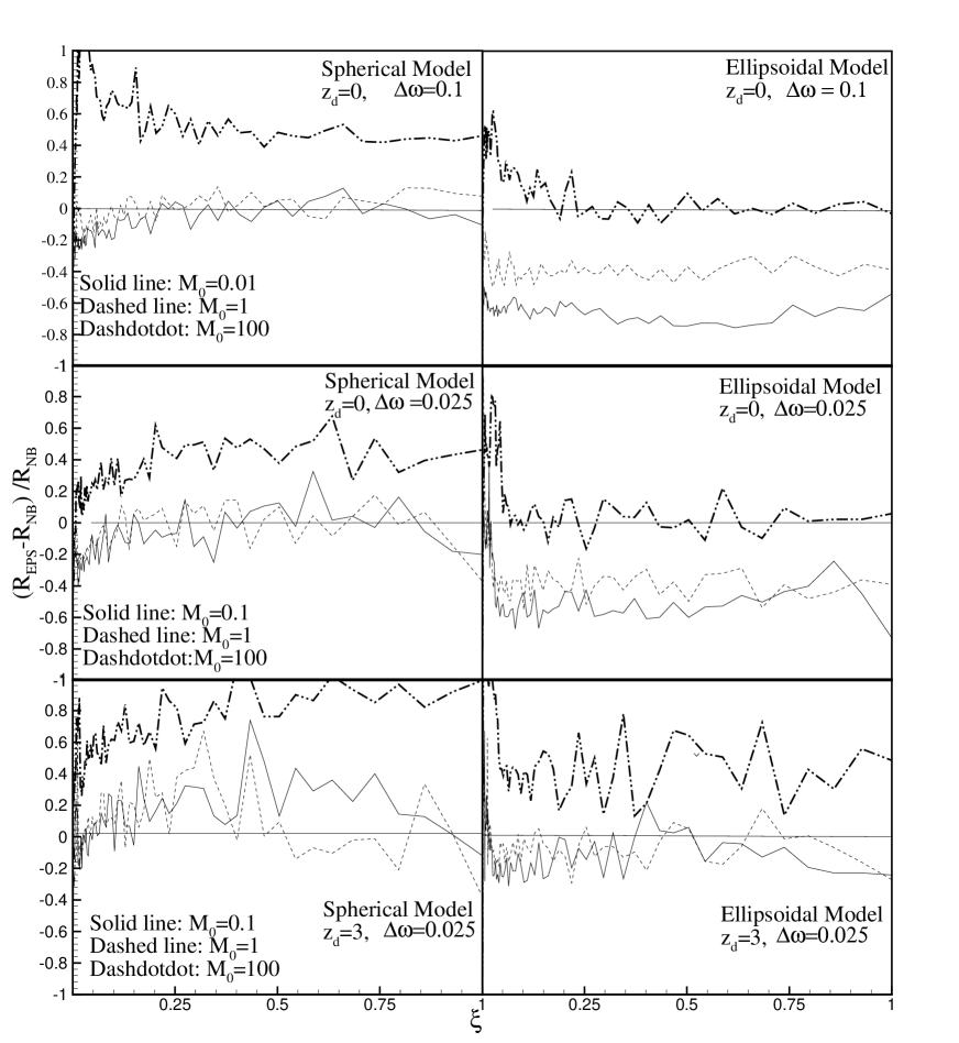
Figure 9: Detailed comparisons between the EPS and N-body results. The relative difference $(R_{EPS}-R_{NB})/R_{NB}$, where $R_{EPS}$ and $R_{NB}$ are the merger rates predicted by the EPS and by N-body results respectively, is plotted as a function of $\xi$. SC model gives merger rates that are in good agreement with N-body results for small haloes (in the range $0.01-1$) while EC model approximates better the merger rates of heavy haloes ($M_{0}=100$).

In Figs 7 and 8 we present results for different masses, redshifts and time-steps. In all snapshots dashed lines are the predictions of the SC model and solid lines show the results of the EC model. Squares are the predictions of the N-body fitting formula formula given by Eq.(13).
From the results presented in the first row of Fig.7 is clear that the EC model results to merger rates that are not in agreement with the results of N-body simulations, for a descendant halo of small mass $M_{0}=0.01$. Instead the results of SC seem to be satisfactory. For larger masses the agreement between EC model and N-body results becomes better. For large haloes, $M_{0}=100$, EC model approximates N-body simulations better than SC model. All the results of Fig.7 have been calculated for $\Delta\omega=0.1$. Fist column shows results for $z_{d}=0$ while the second one for $z_{d}=1$.
All curves in Fig.8 have been predicted for $\Delta\omega=0.025$. Three rows correspond to $M_{0}=0.1,M_{0}=1$ and $M_{0}=100$, respectively. As in Fig.7, different lines represent different models. Thick dashes show the results of SC model, solid line the results of EC model and squares the results of the fitting formula give by Eq. (13).
A more detailed comparison between the results of EPS and N-body simulations is given in Fig.9. We calculated the relative difference $(R_{EPS}-R_{NB})/R_{NB}$ where $R_{EPS}$ and $R_{NB}$ are the merger rates predicted by the EPS and by N-body results, respectively. The results presented in this Fig. can be summarized as follows:
For low redshifts ($z=0$ to $z=1$), merger rates of haloes with descendant mass in the range $10^{10}M_{\odot}\mathrm{h}^{-1}$ to $10^{12}M_{\odot}\mathrm{h}^{-1}$ derived by the SC model fit very satisfactory the results of N-body simulations. For example, for $z_{d}=0$ and $\Delta\omega=1$ the difference is less than $15$ percent, except for some very small values of $x$. Instead, for the same range of masses and redshifts, merger rates derived by the EC are significantly lower than those predicted by N-body simulations.
For the above range of redshifts and for haloes of mass $10^{14}M_{\odot}\mathrm{h}^{-1}$ the fits by EC model are very satisfactory (in general the relative difference is smaller than $20$ percent) while the results of SC are significantly higher than those of N-body simulations.
For a higher redshift ($z=3$) both SC and EC model overestimate the merger rate of large haloes. Merger rates of smaller haloes are overestimated by the SC model and underestimated by the EC model. The above conclusion seems not to depend, at least significantly, on the values of redshift $z_{d}$ and time-step $\Delta\omega$.
We have to note here that both N-body simulations and analytical methods have problems in describing very accurately some physical properties of dark matter haloes. This is due to either technical difficulties or to the fact that some physical mechanisms are not taken into account. For example, in a recent paper Fakhouri & Ma (2010) use the results of the Millenium - II simulation, (Boylan et al., 2009), to derive a formula of the same form of that given in Eq.(13). Millenium - II simulation has better resolution than Millenium, (Springel et al., 2005), simulation. Due to the better resolution, the best fitting values of the parameters in Eq.(13) are changed. For example, the value of $a_{1}$, that is the exponent of the mass of the halo, from $0.083$ becomes now $0.133$. Obviously the dependence of mass remains weak but such a change in the value of $a_{1}$ results, for a halo with $M_{d}=100$, to a new merger rate that is $26\%$ larger. This percentage is too large since it can change the whole picture, at least for large haloes, resulting from our comparison. Additionally, it is interesting to notice Fig. A1 in the appendix of the above paper. It describes merger rates given by five different algorithms. These algorithms are used to analyze the results of the same simulation and to study fragmentation effects in FOF (friends of friends) merger trees. From this Fig. it is clear that differences due the use of different algorithms may be larger than the differences between analytical methods and N-body simulations derived by our study and shown in our Fig.9.
From the above discussion it is clear that the results of N-body simulations are very sensitive not only to the resolution but also to the halo finding algorithm. This sensitivity can lead to completely different results. The following example is very characteristic: Bet et al. (2007) studied, among other things, the value of the spin parameter as a function of the mass of dark matter haloes. They found that the FOF algorithm results to a spin parameter that is an increasing function of mass while a more advanced halo finding algorithm, that they been proposed, results to a spin parameter that is a decreasing function of mass! On the other hand, N-body simulations have the ability to deal with complex physical process. For example the destruction of dark matter haloes as well as the the role of the environment are factors that are not taken into account in most of the analytical methods. This is an additional reason for the presence of differences between the results.
Summarizing our results we could say that: SC approximates better the merger rates of small haloes while EC the merger rates of heavy haloes. This is obviously an interesting information, but since it has been resulted from a specific solution for the problem of the distribution of progenitors, a further study of different solutions is required. The finding of a solution that approximates satisfactory merger rates from N-body simulations, independently on the redshift and mass should be an important achievement. Such a trial requires future comparisons and obviously improvements on both kind of methods.

5 Acknowledgements

We acknowledge K. Konte and G. Kospentaris for assistance in manuscript preparation and the Empirikion Foundation for financial support.

References

- Bet et al. (2007) Bett P., Eke V., Frenk C.S., Jenkins A., Helly J., Navarro J., 2007, MNRAS, 376, 215
- Bond et al. (1991) Bond J.R., Cole S., Efstathiou G., Kaiser N., 1991, ApJ, 379, 440
- Boylan et al. (2009) Boylan-Kolchin M., Springel V., White S.M.D., Jenkins A., Lemson G., 2009, MNRAS, 398,1150
- Fakhouri & Ma (2008) Fakhouri O., Ma C.-P., 2008, MNRAS, 386, 577
- Fakhouri & Ma (2010) Fakhouri O., Ma C.-P., Kolchin M.B., 2010, MNRAS, 406, 226
- Hiotelis & Del Popolo (2006) Hiotelis N., Del Popolo A., 2006, Ap&SS, 301, 167
- Hiotelis (2006) Hiotelis N., 2006, A&A, 315, 191
- Lacey & Cole (1993) Lacey C., Cole S., 1993, MNRAS, 262, 627
- Lin et al. (2003) Lin W.P., Jing Y.P., Lin L., 2003, MNRAS, 344, 1327
- Neinstein & Dekel (2008) Neinstein E., Dekel A., 2008, MNRAS, 388, 1792
- Peebles (1980) Peebles P.J.E. Large Scale Structure of the Universe, 1980, Princeton University Press, Princeton
- Press & Schechter (1974) Press W., Schechter P., 1974, ApJ, 187, 425
- Sheth & Tormen (1999) Sheth R.K., Tormen G., 1999, MNRAS, 308, 119
- Sheth & Tormen (2002) Sheth R.K., Tormen G., 2002, MNRAS, 329, 61
- Smith et al. (1998) Smith C.C., Klypin A., Gross M.A.K., Primack J.R., Holtzman J., 1998, MNRAS, 297, 910
- Somerville & Kollat (1999) Somerville R.S., Kollat T.S., 1999, MNRAS, 305, 1
- Springel et al. (2005) Springel et al., 2005, Nature, 435, 629
- Yahagi et al. (2004) Yahagi H., Nagashima M., Yoshii Y., 2004,ApJ, 605, 709
- van den Bosch (2002) van den Bosch F.C., 2002, MNRAS, 331, 98
- Zhang & Hui (2006) Zhang J., Hui L., 2006, ApJ, 641, 641