Identifying Lagrangian fronts with favourable fishery conditions

Abstract

Lagrangian fronts (LF) in the ocean delineate boundaries between surface waters with different Lagrangian properties. They can be accurately detected in a given velocity field by computing synoptic maps of the drift of synthetic tracers and other Lagrangian indicators. Using Russian ship’s catch and location data for a number of commercial fishery seasons in the region of the northwest Pacific with one of the richest fishery in the world, it is shown statistically that the saury fishing grounds with maximal catches are not randomly distributed over the region but located mainly along those LFs where productive cold waters of the Oyashio Current, warmer waters of the southern branch of the Soya Current, and waters of warm-core Kuroshio rings converge. Computation of those fronts with the altimetric geostrophic velocity fields both in the years with the First and Second Oyashio Intrusions shows that in spite of different oceanographic conditions the LF locations may serve good indicators of potential fishing grounds. Possible reasons for saury aggregation near LFs are discussed. We propose a mechanism of effective export of nutrient rich waters based on stretching of material lines in the vicinity of hyperbolic objects in the ocean. The developed method, based on identifying LFs in any velocity fields, is quite general and may be applied to forecast potential fishing grounds for the other pelagic fishes in different seas and the oceans.

PRANTS ET AL. IDENTIFYING LAGRANGIAN FRONTS S. V. Prants, prants@poi.dvo.ru

1 Introduction

Regions, where horizontal gradients of hydrological properties go through a maximum, are ubiquitous in the ocean. The importance of oceanic fronts to ecosystems may be explained by the fact that they are associated with a convergent flow with an intensified flux of nutrients. If the front is sufficiently long-lived, populations of phyto- and zooplankton will increase attracting the other higher level organisms in the trophical chain which are able to detect the front.

By the common opinion (Owen, 1981; Olson et al., 1994; Bakun, 2006), good fishing areas are often found at the boundaries of warm and cold currents and around warm-core eddies where the energy of the physical system is transferred in some way to biological processes. This strong physical-biological interaction provides favourable conditions for marine organisms. Surface convergent fronts of considerable physical and biological activity occur in zones where different water types impinge. The reasons leading to aggregation of tuna, saury and some other pelagic fishes at oceanic fronts are unknown in detail, but there are in the literature some speculations about physical mechanisms providing a transfer of the energy of the physical system to biological processes (Owen, 1981; Olson et al., 1994; Bakun, 2006). They include transport of nutrients, phytoplankton blooms and aggregation of other marine organisms at fronts and eddy edges. Thus, oceanic fronts work as aggregating mechanisms for zooplankton, the main food for pelagic fishes. SST gradients have long been the main indicators used to find places in the ocean with rich marine resources.

In the northwest Pacific, the cold Oyashio Current flows out of the Arctic along the Kamchatka Peninsula and the Kuril Islands and converges with the warmer Kuroshio Current off the eastern shore of Japan. This frontal zone is known to be one of the richest fishery in the world due to the large nutrient content in the Oyashio waters and high tides in some areas therein. Some people attempted to identify the favourable oceanographic conditions for catching pelagic fishes. The Kuroshio-Oyashio fronts have long been recognised by Japanese fishermen to attract squids, fishes and mammals (for the earlier studies see Ref. (Uda, 1938)). It was found that fishing grounds depend on the location of the Oyashio fronts and vary from year to year (Fukushima, 1979; Saitoh et al., 1986; Sugimoto and Tameishi, 1992; Yasuda and Kitagawa, 1996). The fishing grounds are located near shore if there exists the First Oyashio Intrusion along the eastern coast of Hokkaido, Japan. In the other years, the fishing grounds are located offshore where the Second Oyashio Intrusion is formed due to the presence there of a large warm-core Kuroshio ring. It has been shown that locations of the fishing grounds depend not only on instantaneous and local oceanographic conditions nearby the fishing grounds but on the conditions over the whole region.

We study here the connection of Lagrangian fronts (LFs), delineating boundaries between surface waters with different Lagrangian properties, and fishing grounds. To be concrete, we focus on fishing grounds of Pacific saury (Cololabis saira), one of the most commercial pelagic fishes in the region. The Pacific saury is a migratory pelagic fish moving in schools. They used to pass for 5 – 6 months distances of the order of 2500 miles from spawning grounds to feeding grounds. They spend much of the time near the surface in nights and in deeper waters in daily time. Pacific saury, in general, migrate seasonally from the south to the north. In winter and spring, spawning grounds are formed in the south, off the eastern coast of Honshu, Japan. In spring and summer, juvenile and young saury migrate northward to the Oyashio area. After feeding in those productive waters, adult saury migrate to the south in the late summer. Commercial fishery begins in August and ends in December.

Based on the AVISO altimetric geostrophic velocity fields, we compute synoptic maps of zonal, meridional, and absolute drift of synthetic tracers and the finite-time Lyapunov exponents (FTLE). Those maps with the catch data from the Russian saury fishery overlaid allow to identify the LFs in the region with favourable fishing conditions in the years both with the First and Second Oyashio Intrusions. In order to determine whether saury is actively associating with LFs or not, we compute the frequency distributions of the distances between locations of fishing boats with saury catches and the LFs. The comparison of those distributions with random distributions of fishing boats over the same region for all the fishery seasons with available data provides evidence that saury fishing locations are not randomly distributed over the region but congregate near strong LFs. Thus, the LFs may serve as a new indicator for potential fishing grounds.

The paper is organized as follows. Section 2 gives an introduction to the Lagrangian approach to study transport and mixing in the ocean based on application and elaboration of some methods from dynamical systems theory. Section 3 details the data and methods used in the paper. We introduce there the notion of a LF and discuss briefly their specifics and difference from common oceanic fronts and Lagrangian coherent structures. Section 4 contains the illustrative examples on identification of LFs favourable for saury fishing in the seasons with the First and Second Oyashio Intrusions in the region to the east off Hokkaido and southern Kuril Islands coasts. The representative drift and FTLE synoptic maps for two different oceanographic situations in the region are demonstrated in that section. The quantitative results are presented in section 5 where it is shown statistically that the saury fishing grounds with maximal catches are not randomly distributed over the region but located mainly near strong LFs. In Appendix, we describe our method to compute accurately the FTLE.

2 Lagrangian approach to study transport and mixing in the ocean

Motion of a fluid particle in a two-dimensional flow is the trajectory of a dynamical system with given initial conditions governed by the velocity field. The corresponding advection equations are written as follows:

$$\frac{dx}{dt}=u(x,y,t),\quad\frac{dy}{dt}=v(x,y,t),$$ (1)

where the longitude, $x$, and the latitude, $y$, of a passive particle are in geographical minutes, $u$ and $v$ are angular zonal and meridional components of the velocity expressed in minutes per day. Even if the Eulerian velocity field is fully deterministic, the particle’s trajectories may be very complicated and practically unpredictable. It means that a distance between initially close fluid particles grows exponentially in time

$$\|\delta{\mathbf{x}}(t)\|=\|\delta{\mathbf{x}}(0)\|\,e^{\Lambda t},$$ (2)

where $\Lambda$ is a positive number, known as the maximal Lyapunov exponent, which characterizes asymptotically the average rate of the particle dispersion, and $\|\mathbf{x}\|$ is a norm of the vector $\mathbf{x}=(x,y)$. It immediately follows from (2) that we are unable to forecast the fate of the particles beyond the so-called predictability horizon (Koshel’ and Prants, 2006)

$$T_{p}\simeq\frac{1}{\Lambda}\ln\frac{\|\Delta\|}{\|\Delta(0)\|},$$ (3)

where $\|\Delta\|$ is the confidence interval of the particle location and $\|\Delta(0)\|$ is a practically inevitable inaccuracy in specifying the initial location. The deterministic dynamical system (1) with a positive maximal Lyapunov exponent for almost all vectors $\delta\mathbf{x}(0)$ (in the sense of nonzero measure) is called chaotic. It should be stressed that the dependence of the predictability horizon $T_{p}$ on the lack of our knowledge of exact location is logarithmic, i. e., it is much weaker than on the measure of dynamical instability quantified by $\Lambda$. Simply speaking, with any reasonable degree of accuracy on specifying initial conditions there is a time interval beyond which the forecast is impossible, and that time may be rather short for chaotic systems.

Since the phase plane of the two-dimensional dynamical system (1) is the physical space for fluid particles, many abstract mathematical objects from dynamical systems theory (fixed points, Kolmogorov–Arnold–Moser tori, stable and unstable manifolds, periodic and chaotic orbits, etc.) are material surfaces, curves and points in fluid flows (for a review see (Wiggins, 2005; Koshel’ and Prants, 2006)). It is well known that besides “trivial” elliptic fixed points, the motion around which is stable, there are hyperbolic fixed points which organize fluid motion in their neighbourhood in a specific way. In a steady flow the hyperbolic points are typically connected by the separatrices which are their stable and unstable invariant manifolds. In a time-periodic flow the hyperbolic points are replaced by the corresponding hyperbolic trajectories with associated invariant manifolds which in general intersect transversally resulting in a complex manifold structure known as homo- or heteroclinic tangles. The fluid motion in these regions is so complicated that it may be strictly called chaotic, the phenomenon known as chaotic advection (for a review see (Koshel’ and Prants, 2006)). Adjacent fluid particles in such tangles rapidly diverge providing very effective mechanism for mixing.

Stable and unstable manifolds are important organizing structures in the flow because they attract and repel fluid particles (not belonging to them) and partition the flow into regions with quantitatively different types of motion. Invariant manifold in a two-dimensional flow is a material line, i. e., it is composed of the same fluid particles in course of time. By definition (Wiggins, 2005; Koshel’ and Prants, 2006), stable ($W_{s}$) and unstable ($W_{u}$) manifolds of a hyperbolic trajectory $\gamma(t)$ are material lines consisting of a set of points through which at time moment $t$ pass trajectories that are asymptotical to $\gamma(t)$ at $t\to\infty$ ($W_{s}$) and $t\to-\infty$ ($W_{u}$). They are complicated curves infinite in time and space that act as boundaries to fluid transport.

The real oceanic flows are not, of course, strictly time-periodic. However, in aperiodic flows there exist under some mild conditions hyperbolic points and trajectories of a transient nature. In aperiodic flows it is possible to identify aperiodically moving hyperbolic points with stable and unstable effective manifolds (Haller and Yuan, 2000). Unlike the manifolds in steady and periodic flows, defined in the infinite time limit, the “effective” manifolds of aperiodic hyperbolic trajectories have a finite lifetime. The point is that they play the same role in organizing oceanic flows as do invariant manifolds in simpler flows (Haller and Poje, 1998; Haller and Yuan, 2000; Haller, 2000). The effective manifolds in course of their life undergo stretching and folding at progressively small scales and intersect each other in the homoclinic points in the vicinity of which fluid particles move chaotically. Trajectories of initially close fluid particles diverge rapidly in these regions, and particles from other regions appear there. It is the mechanism for effective transport and mixing of water masses in the ocean. Moreover, stable and unstable effective manifolds constitute Lagrangian transport barriers between different regions because they are material invariant curves that cannot be crossed by purely advective processes.

The stable and unstable manifolds of influential hyperbolic trajectories are so important because (1) they form a kind of a template around which oceanic flows are organized, (2) they divide a flow in dynamically different regions, (3) they are in charge of forming an inhomogeneous mixing with spirals, filaments and lobes, (4) they are transport barriers separating water masses with different characteristics. Stable manifolds act as repellers for surrounding waters but unstable ones are attractors. That is why unstable manifolds may be rich in nutrients being oceanic “dining rooms”.

To quantify chaos in dynamical systems, one computes the maximal Lyapunov exponent which enables to detect and visualize stable and unstable manifolds as well. In aperiodic flows, it is instructive to use with these aims the FTLE that is the finite-time average of the maximal separation rate for a pair of neighbouring advected particles. This quantity can be computed accurately by the method introduced in Ref. (Prants et al., 2011a).

3 Data and Methods

The general method we used is based on the Lagrangian approach to study mixing and transport at the sea surface (Haller and Poje, 1998; Haller and Yuan, 2000; Haller, 2000; Boffetta et al., 2001; Mancho et al., 2004; d’Ovidio et al., 2004; Shadden et al., 2005; Kirwan Jr., 2006; Lehahn et al., 2007; Beron-Vera et al., 2008; Prants et al., 2011a, b, 2013) when one follows fluid particle trajectories in a velocity field calculated from altimetric measurements or obtained as an output of one of the ocean circulation model. The important notion in that approach is so-called Lagrangian coherent structures (LCS) (Haller and Poje, 1998; Haller and Yuan, 2000; Haller, 2000). The well-known coherent structures in the ocean are eddies and jet currents that can be visible in Eulerian velocity fields and at satellite images of the SST and/or chlorophyll concentration. The LCSs, in general, are not visible at snapshots but can be computed with a given velocity field by special methods. Lagrangian coherent structures are operationally defined as local extrema of the scalar FTLE field (Haller and Poje, 1998; Haller and Yuan, 2000; Haller, 2000). They are the most influential attracting and repelling hyperbolic material surfaces which are curves in 2D velocity fields. The LCS are Lagrangian because they are invariant material curves consisting of the same fluid particles. They are coherent because they are comparatively long lived and more robust than the other adjacent structures. The LCS are connected with the effective stable and unstable invariant manifolds of hyperbolic (unstable) trajectories that can be approximately identified with the help of the FTLE and other Lagrangian indicators, hyperbolicity time (Haller and Yuan, 2000), patchiness (Lukovich and Shepherd, 2005), the so-called M-function which measures the Euclidean arc-length of the curves outlined by trajectories for a finite-time interval (Mendoza and Mancho, 2010), the correlation dimension of trajectory and the so-called ergodicity defect (Rypina et al., 2011). A new approach to locating material transport barriers in unsteady planar fluid flows has been introduced recently (Haller, 2011; Haller and Beron-Vera, 2012). Seeking transport barriers as minimally stretching material lines, it is possible to locate hyperbolic barriers (generalized stable and unstable manifolds), elliptic barriers (generalized KAM curves) and parabolic barriers (generalized shear jets) in temporally aperiodic flows defined over a finite time interval. This approach (Haller, 2011; Haller and Beron-Vera, 2012) also yields a metric (geodesic deviation) that determines the minimal computational time scale needed for a robust numerical identification of generalized LCSs.

The convenient measures to distinguish trajectories with different particle’s fate and origin have been introduced recently, namely, the time particles need to leave a given region (Prants et al., 2011a), absolute, zonal, and meridional displacements of particles from their initial positions (Prants et al., 2011b, 2013). The impact of LCSs on biological organisms has been recently studied in Ref. (Tew Kai et al., 2009). By comparing the seabird satellite positions with computed LCSs locations, it was found that a top marine predator, the Great Frigatebird, was able to track the LCSs in the Mozambique Channel identified with the help of the finite-size Lyapunov exponent.

The LCSs are determined mainly by the large-scale advection field, which is appropriately captured by altimetry. It has been shown theoretically (Haller, 2002) that the LCSs are robust to errors in observational or model velocity fields if they are strongly attracting or repelling and exist for a sufficient long time. This is due to the fact that though the particle trajectories will in general diverge exponentially from the true trajectories near a repelling LCS, the very LCSs are not expected to be perturbed to the same degree, because errors in the particle trajectories spread along the LCS. A few numerical experiments have been carried out to test the sensitivity of LCSs, found by identifying ridges of the FTLE, to errors in altimetric velocity fields. LCS were found to be relatively insensitive to both sparse spatial and temporal resolution and to the velocity field interpolation method (Harrison and Glatzmaier, 2012; Keating et al., 2011; Hernández-Carrasco et al., 2011). The FTLE method is reliable for locating boundaries of large eddies and strong jets. However, small LCS features are not well resolved from altimetry and should be considered with some caution. The comparison of the LCSs computed with altimetric velocity fields in numerous paper (see, for example, (Abraham and Bowen, 2002; Olascoaga et al., 2006; Beron-Vera et al., 2008; d’Ovidio et al., 2009; Huhn et al., 2012)) with independent satellite and in situ measurements of thermal and other fronts in different seas and oceans has been shown a good correspondence.

Our approach is based on searching for specific Lagrangian features in the altimetric geostrophic velocity fields which indicate to the presence of convergence of waters with different properties. We call them Lagrangian Fronts (LF), which are boundaries between surface waters with different Lagrangian properties. It may be, for example, a thermodynamical property, such as SST, salinity, density, etc. or concentration of chlorophyll-a. Lateral maximal gradients of those properties would indicate on common oceanic fronts, thermal, salinity, density and chlorophyll ones, which are often connected with each other. However, one may consider more specific Lagrangian indicators which are functions of a particle’s trajectory, such as a distance passed for a given time, absolute, meridional, and zonal displacements of particles from their initial positions, the numbers of their cyclonic and anticyclonic rotations, etc. Even in the situation where the water itself is indistinguishable, say, in temperature, and the corresponding SST image does not show a thermal front there may exist a LF separating waters with the other distinct properties.

Common oceanic fronts are manifestations of the current state of a water medium that can be detected by direct measurements. SST and ocean color fronts are visible on satellite images which, however, are not available in cloudy or rainy days. The LFs reflect history and origin of water masses and can be computed and visualized on Lagrangian maps. They can be, in principle, measured by launching a large number of drifters in appropriate places. The LFs may coincide with common oceanic fronts but may not. It is possible to compute the LF of such a Lagrangian indicator that would not manifest itself as an oceanic front but would give a useful information on water motion. Even if a specific LF does not coincide with a common oceanic front, it does not mean that it would be usefulness. Such the LF may simply reflect the other properties of convergent water masses

The relationship between LCSs and LFs is not trivial. Any LF by definition is a curve with the maximal local gradient of a Lagrangian property which varies significantly on both sides of the LF, whereas the FTLE values are almost the same on both sides of any ridge in the FTLE field defining a LCS. By definition, any Lagrangian indicator is a function of trajectory, whereas in order to compute the FTLE it is necessary in addition to know the dynamical system as well. LCSs contain information about evolution of some medium segments. The drift and the other Lagrangian indicators are characteristics of a given fluid particle whereas the Lyapunov exponent is a characteristic of the medium surrounding that particle. Moreover, LCSs and LFs have a different topology on Lagrangian maps, the first ones are 2D bands (ridges) whereas the latter ones are curves (gradients). We would like to stress the important role of the LFs because, in difference from rather abstract geometric objects of an associated dynamical system, like invariant manifolds, $W_{s}$ and $W_{u}$, they are fronts of real physical quantities that can be, in principle, measured.

Of particular importance in detecting LFs is the drift, $D$, that is simply the distance between the final, $(x_{f},y_{f})$, and initial, $(x_{0},y_{0})$, positions of advected particles on the Earth sphere with the radius $R$

$$D\equiv R\arccos[\sin y_{0}\sin y_{f}+\cos y_{0}\cos y_{f}\cos(x_{f}-x_{0})],$$ (4)

This quantity and zonal, $D_{x}$, and meridional, $D_{y}$, drifts have been shown to be useful in quantifying transport of radionuclides in the Northern Pacific after the accident at the Fukushima atomic plant station (Prants et al., 2011b) and transport of the Madagascar plankton bloom (Huhn et al., 2012).

The FTLE field characterizes quantitatively mixing along with directions of maximal stretching and contracting, and it is applied to identify LCSs in irregular velocity fields. The FTLE is computed here by the method of the singular-value decomposition of an evolution matrix for the linearized advection equations (Prants et al., 2011a) and is given by formulae (for details see Appendix)

$$\lambda(t,t_{0})=\frac{\ln\sigma(t,t_{0})}{t-t_{0}},$$ (5)

which is the ratio of the logarithm of the maximal possible stretching in a given direction to a time interval $t-t_{0}$. Here $\sigma(t,t_{0})$ is the maximal singular value of the evolution matrix. The method proposed enables to compute accurately the FTLE in altimetric velocity fields.

Geostrophic velocities were obtained from the AVISO database (http://www.aviso.oceanobs.com). The data is gridded on a $1/3^{\circ}\times 1/3^{\circ}$ Mercator grid. Bicubical spatial interpolation and third order Lagrangian polynomials in time have been used to provide accurate numerical results. Lagrangian trajectories have been computed by integrating the advection equations with a fourth-order Runge-Kutta scheme with a fixed time step of $0.001$th part of a day.

The SST data (http://oceancolor.gsfc.nasa.gov) were used to illustrate oceanographic conditions in the cases of the First and Second Oyashio Intrusions. The data on fishing positions in latitude and longitude and daily catches were obtained from the database of the Federal Agency for Fishery of the Russian Federation.

4 Results

4.1 Identification of the Lagrangian fronts favourable for saury fishing in the season with the First Oyashio Intrusion

We restrict our analysis in this paper by the region to the east off Hokkaido (Japan) and southern Kuril Islands (Russia) coasts where the daily saury catch data from the Russian fishery were collected for a few fishery seasons. With the aim to detect the LFs separating waters with different origin and histories, we distribute a large number of synthetic particles over that region and integrate advection equations (1) backward in time for two weeks to compute the zonal, $D_{x}$, meridional, $D_{y}$, and absolute, $D$, particle’s displacements from their positions on the initial day. Coding the particle’s displacements by color, one gets the synoptic maps that provide the evidence of origin of water masses present in the region on a given day.

In some seasons there exists the First Oyashio Intrusion along the eastern coast of Hokkaido which is visible on the SST image in Fig. 1a averaged for 23–25 September 2002. It is a combined map with the velocity field specified by arrows, contour lines of the FTLE, $\lambda$, and locations of “instantaneous” hyperbolic (crosses) and elliptic (triangles) fixed points imposed. Blue and red triangles mean cyclonic and anticyclonic rotations, respectively. The data of saury catch for 23–25 September 2002 overlaid allow to conclude that the fishery grounds have been concentrated in the waters of the First Oyashio Intrusion (the radius of the circles in the figure is proportional to the catch in tons per a given ship). In Fig. 1b the vorticity field, $\operatorname{rot}\mathbf{v}$, together with the velocity field, $\mathbf{v}=(u,v)$, are shown on 24 September 2002 with the locations of “instantaneous” hyperbolic (crosses) and elliptic (triangles) fixed points imposed. The region contains a number of the vorticity patches with cyclonic (blue) and anticyclonic (red) rotations.

Computing backward in time the displacements for a large number of particles from their initial to final positions, we get the zonal, $D_{x}$, and meridional, $D_{y}$, drift maps with the contour lines of the FTLE and the black circles of saury catch locations imposed. Those maps visualize clearly the LFs with convergent water masses with different origin and histories. The color on the zonal drift map (Fig. 1c) distinguishes the particles entering to the region through its western (red) and eastern (green) boundaries whereas red and green colors on the meridional drift map (Fig. 1d) mean that particles enter to the region through its southern and northern boundaries, respectively. Nuances of the color on both the figures code the distance passed by the corresponding particles in the zonal or meridional directions in degrees. It is seen on both the drift maps that productive cold waters of the Oyashio Current and warmer waters of the southern branch of the Soya Current flowing through the straights between the southern Kuril Islands converge at the LFs with the maximal catches. This LF demarcates the boundary between the “green” and “red” waters. The absolute drift map, $D(x,y)$, in Fig. 1e confirms this conclusion visualizing the same LF with maximal catches (yellow circles) as a boundary between “dark” and “grey” waters.

In Fig. 1f we show the FTLE field on 24 September 2002, computed by the method described in Appendix, with the contours of the particle’s absolute drift $D$. The black “ridges” (curves of the local maxima) of that field are known to delineate stable manifolds of the most influential hyperbolic trajectories in a region when integrating advection equations forward in time and unstable ones when integrating them backward in time. The black “ridges” on the map in Fig. 1f delineate the corresponding unstable manifolds which are by definition the curves of maximal stretching. The adjacent particles, belonging to them, may have a different history because the larger the FTLE value the larger is an initial distance between the corresponding particles (backward-in-time integration). The particles with maximal FTLE came to their locations from very different places. Thus, the black “ridges” of the FTLE field demarcate approximately the corresponding LFs (compare Figs. 1e and f). On the other hand, there exist the LFs that are not connected with FTLE “ridges”. Animation of the daily Lagrangian maps for August – December 2002 with the fishery grounds overlaid is available at http://dynalab.poi.dvo.ru/data/GRL12/2002.

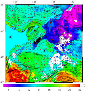
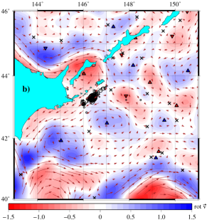
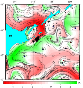
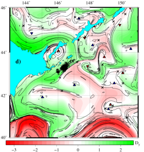
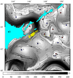
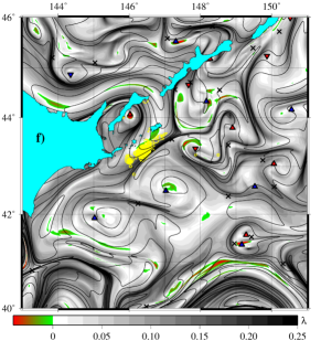
Figure 1: The season with the First Oyashio Intrusion. (a) SST image, (b) vorticity map, (c) zonal, (d) meridional, and (e) absolute drift maps, and (f) FTLE map on 24 September 2002 with locations of saury catches imposed. FTLE is in units of $[\rm days]^{-1}$, the zonal and meridional drifts, $D_{x,y}$, are in degrees, and the absolute drift, $D$, is in km. See explanation in the text.

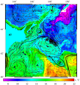
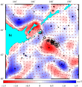
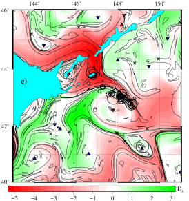
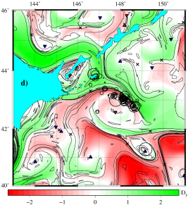
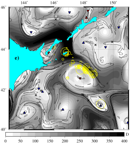
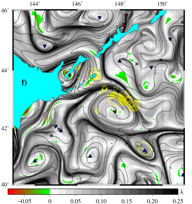
Figure 2: The season with the Second Oyashio Intrusion. (a) SST image, (b) vorticity map, (c) zonal, (d) meridional, and (e) absolute drift maps, and (f) FTLE map on 17 October 2004 with locations of maximal saury catches imposed.

4.2 Identification of the Lagrangian fronts favourable for saury fishing in the season with the Second Oyashio Intrusion

The oceanographic situation in the region cardinally differs in the years with the Second Oyashio Intrusion when a large anticyclonic eddy, formed as a warm-core Kuroshio ring, approaches to the Hokkaido eastern coast and forces the Oyashio Current to shift to the east rounding the eddy. The SST image in Fig. 2a averaged for 16–18 October 2004 demonstrates that the fishery grounds have been concentrated mainly at the convergence front between the Oyashio and Soya waters and the periphery of the anticyclonic Kuroshio ring with the center around $x_{0}=147^{\circ}30^{\prime}$E, $y_{0}=42^{\circ}30^{\prime}$N.

The vorticity map in Fig. 2b demonstrates that the maximal saury catch spots are concentrated around the northeastern edge of the warm anticyclonic Kuroshio ring, the big red spot with the center around $x_{0}=147^{\circ}30^{\prime}$E, $y_{0}=42^{\circ}30^{\prime}$N. The zonal, meridional, and absolute drift maps on the same date in Figs. 2c, d, and e with the circles of saury catch locations overlaid show clearly that the fishery grounds with maximal catches are located along the LFs where productive cold waters of the Oyashio Current, warmer waters of the southern branch of the Soya Current and warm and salty waters of the Kuroshio ring converge. The FTLE map in Fig. 2f on 17 October 2004 demonstrates that the fishery grounds are located along the three main unstable manifolds in the region which demarcate approximately the corresponding LFs. Animation of the daily Lagrangian maps for August – December 2004 with the fishery grounds overlaid is available at http://dynalab.poi.dvo.ru/data/GRL12/2004.

5 Frequency distribution of the distances between fishing boats with catches and Lagrangian fronts

We demonstrated above a relationship between LFs and locations of fishing boats with saury catches in different oceanographic situations. In order to determine quantitatively whether saury is actively associating with the LFs in the region studied or not, we compute the frequency distribution of the distances, $r$, between locations of fishing boats with saury catches and the strong LFs for available fishery seasons. The maximal gradient of the absolute displacement, $\nabla D=\sqrt{(\partial D/\partial x)^{2}+(\partial D/\partial y)^{2}}$, is supposed to be an identificator of the presence of a LF. Such gradients delineate boundaries between waters that passed distances that may differ in two orders of magnitude (see Figs. 1e and 2e). It has been shown in Sec. 4 that the contrast boundaries are the strongest LFs separating productive cold waters of the Oyashio Current, warmer waters of the southern branch of the Soya Current, and waters of warm-core Kuroshio rings. In order to get rid of ephemeral LFs, we choose a threshold, $\nabla D_{\rm th}=60$, and only the LFs with $\nabla D_{\rm th}\geq 60$ are supposed to be “strong”. We have found that such gradient values correspond to permanent LFs in the Kuroshio–Oyashio frontal area. Then we compute on each day the distance $r$ between the location of each boat with saury catch and the nearest geographical point where $\nabla D_{\rm th}\geq 60$. The corresponding probability distribution function (PDF) for each season is compared with the random PDF which is computed by the same way but with 10000 points randomly distributed over the same region. The fishery strategy depends on the oceanographic situation in the region, captain’s experience, other subjective factors and varies during the fishery period. As a rule, the Russian captains begin to catch saury in July – August in the northern part of the region studied where saury schools start their migration to the south. It is profitable to begin the fishery nearby the ports on the southern Kuril Islands. The fishing grounds there are connected rather with the strong upwelling due to high tides than with LFs. Then, in September, the fishing boats moved to the south following the saury schools. By safe and another reasons, the boats prefer to stick together. After reporting by one of them a good catch, the other ones may move to that place if they were hereabout. The combination of different factors in the fishery strategy, including the subjective ones, makes it difficult to find statistically significant correlations between locations of fishing boats with saury catches and any oceanic features. After all, even if we were able to find precisely potential fishing grounds with favourable hydrological conditions, it would not necessarily implies good real catching if saury or fishing boats do not reach the place.

The results of our statistical analysis are shown in Fig. 3 for all available fishery seasons. The number of events, i. e., the number of locations of the boats with saury catches, varies from season to season and in average was about 1000 per season. As expected, the random PDFs (thin curves) are rather smooth curves with long tails. The real PDFs (bold curves) have a tooth-like structure that can be explained partly by congregation of boats near strong LFs with large $D$ gradients and partly by the fishery strategy to stick together. The vertical solid and dashed lines represent the medians for real and random PDFs, respectively. By definition, the median of a finite list of numbers can be found by arranging all the observations from lowest value to highest one and picking the middle one. It is such a location value that there exists in the list the same number of locations smaller and larger than the median value. The median is a more robust statistical indicator than the mean value and can be used as a measure of location when a distribution is skewed having, for example, a heavy tail. In all the seasons the medians were closer to the LFs for the real PDFs than for the corresponding random ones. Moreover, the random PDFs have more longer tails than the corresponding real ones proving that the fishing boats really tend to be closer to the LFs then be randomly distributed over the region. The plot in Fig. 4 demonstrates the relations between medians (stars) for the real and random PDFs and between mean values (crosses) for the real and random PDFs. In order to take into account the effect of a choice of the threshold value for the displacement gradients, $\nabla D_{\rm th}$, we compute the median and mean values for all the seasons at $\nabla D_{\rm th}=$60, 100, and 130. The points below the slope line in Fig. 4 give evidence that the corresponding median or mean value is closer to LFs for the real fishing boats, $r_{b}$, than for the randomly distributed ones, $r_{r}$. It is evident that both the medians and mean values are closer to LFs in the first case.

The oceanographic situation in 2002 was not typical being the single fishery season, among the studied ones, with the First Oyashio Intrusion. Moreover, the oceanographic situation in the region have changed significantly during that season. Animation of daily Lagrangian maps in 2002 with the fishery grounds overlaid (http://dynalab.poi.dvo.ru/data/GRL12/2002) demonstrates clearly that in addition to the intrusion of Soya Current waters along the north-eastern coast of Hokkaido island there appeared in October – November the intrusion of cold Oyashio waters from the north into the fishery region which cardinally changed the oceanographic situation. The fishery grounds moved to the east and south in that time. The most stable oceanographic situation among the years with available fishery data was in the year 2004 with the Second Oyashio Intrusion, when the quasistationary warm Kuroshio anticyclonic ring was situated in the region for the whole fishery period. The strong LFs have been found to be the permanent ones in that year. The real PDF in Fig. 3 in 2004 exceeds significantly the random one and decays rapidly. The tail of the random PDF extends significantly over the distance $r$ as compared with the real one. All these facts prove that saury fishing grounds really were located mainly along the strong LFs in that year. In the other years with available fishery data, the oceanographic situations resemble the 2004 case with the Second Oyashio Intrusion. Probability distribution functions for those fishery seasons in Fig. 3 provide the statistical evidence that saury fishing locations are not randomly distributed over the region but are concentrated near the strongest LFs around the Kuroshio ring (see Fig. 2). Based on statistical results, we may conclude that the more stable the oceanographic situation in the fishery region is, the closer fishing boats to LFs tend to be.

Figure 3: PDFs for six fishery seasons with real locations of the fishing boats with saury catches (solid curves) and the points randomly distributed over the same region (dashed curves).

Oceanic fronts are areas with strong horizontal and vertical mixing. Highly turbid waters, however, are unsuitable for saury because it is a visual predator hunting in comparatively clear waters outside the exact locations of fronts. They avoid highly turbid waters and waters with large phytoplankton concentration, more than 5 g/m³, which are turbid due to organic matter. On the other hand, extremely oligotrophic waters contain little food. Food abundance and water clarity are known to be two factors affecting the rate of food encounter (Fukushima, 1979; Saitoh et al., 1986; Sugimoto and Tameishi, 1992; Yasuda and Kitagawa, 1996).

Figure 4: Median (stars) and mean (crosses) values for locations of real boats, $r_{b}$, vs randomly distributed ones, $r_{r}$.

As to physical and biological reasons that may cause saury aggregation near LFs, we suggest the following ones. Lagrangian Fronts in the Kuroshio–Oyashio frontal area demarcate the convergence of water masses with different productivity. They are zones with increased lateral and vertical mixing and often with increased primary and secondary production. Mixture of nutrient rich Oyashio waters with more oligotrophic Kuroshio waters can locally simulate phytoplankton photosynthesis and thus sustains higher phyto- and zooplankton concentrations with a net effect of aggregation of saury to forage on the lower trophic level organisms. Stretching of material lines in the vicinity of hyperbolic objects in the ocean, a hallmark of chaotic advection (for a review see (Wiggins, 2005; Koshel’ and Prants, 2006)), is one of the possible mechanisms providing effective intrusions of nutrient rich Oyashio cold waters into more oligotrophic Kuroshio warm waters. Those filament-like intrusions may expand over hundreds of kilometers and are easily captured by the Lagrangian diagnostics but may be not visible on SST or chlorophyll-a images.

We illustrate that mechanism of transport of nutrients in Fig. 5 where evolution of the patches with synthetic particles selected on September 15, 2004 at 5 hyperbolic trajectories in the region is shown. It is the fishery season with the Second Oyashio Intrusion and a prominent quasistationary Kuroshio warm anticyclonic ring in the region (Fig. 2). Let us suppose that some of the patches are rich in food and trace their evolution. Comparing Fig. 5 with the backward-time FTLE map in Fig. 2f, it becomes clear that all the patches in the course of time delineate the corresponding ridges on the map which approximate the unstable manifolds of selected 5 hyperbolic trajectories. The passive marine organisms in those fluid patches have been advected along with them attracting saury for feeding. The perimeter of some patches increased more than in 100 times for only two weeks increasing significantly the chance for saury to find food. Such a mechanism of export of nutrient rich waters into more poor ones is supposed to be typical because of a large number of hyperbolic trajectories in the frontal oceanic zones with increased mixing activity and rich in eddies.

Figure 5: Evolution of the synthetic food patches selected at 5 hyperbolic trajectories in the 2004 fishery season with the Second Oyashio Intrusion. For two weeks the patches delineate rapidly the corresponding unstable manifolds (the black ridges on the FTLE map in Fig. 2f) around the Kuroshio warm ring.

Generally speaking, LFs are 3D features. Lagrangian maps allow to visualize their manifestations at the ocean surface. They may expand over hundreds of kilometers, but fish is expected to aggregate only near comparatively small LF segments. Saury, as a predator of zooplankton, prefer the places with an aggregation of forage zooplankton. Favourable fishing grounds may differ from the adjacent ones by a complex of conditions including hydrological situation in the upper ocean layer. It has been empirically found (Filatov, 2005) that there should be a sharp seasonal termocline (with the vertical gradient more than 0.19^∘ C/m), coinciding in that region with a seasonal pycnocline. Moreover, the width of the upper mixed layer should be more than 6 m with the forage zooplankton concentration more than 0.4 g/m³ but the phytoplankton concentration less than 5.6 g/m³. Such conditions are expected to be formed at LFs where water masses of different densities meet. The heavy cold water tends to flow under the light warm water resulting in formation of a sharp pycnocline which in turn force passive phytoplankton to concentrate all time near the surface but not to be distributed over the depth. Zooplankton is able to move vertically concentrating near the surface in the nighttime. The absolute values of SST in the locations with saury aggregation may vary from 5 to $20^{\circ}$ C. The impoprtant factors of favourable fishery conditions are thermostructural peculiarities and the adundance in forage zooplankton but not SST, salinity and other hydrographic factors.

In the end of this section we would like to discuss the connection between potential fishing grounds, LFs and thermal fronts visible on SST images. SST fronts have long been the main indicators used to find places in the ocean with rich marine resources. So, in order to find potential fishing grounds, it is instructive to use as the first guess the strong thermal gradients visible on satellite SST images if they are available. Unfortunately, SST images are not available in cloudy and rainy days which often occur in the fishery period in the region studied. In some fishery seasons in the Kuroshio–Oyashio frontal area up to half of days have been found to be cloudy or rainy. Typically, the saury fishing grounds with maximal catches have been found not exactly at the SST fronts but in a comparatively large area around that front where a few LFs may be detected. Computation of LFs is a simple way to visualize a fine structure of the frontal zone which is a problem when using SST and/or chlorophyll-a images. Any strong large-scale LFs can be accurately detected in a given altimetric geostrophic velocity field by computing synoptic maps of the drift of synthetic tracers. Moreover, by computing meridional and zonal drift maps, one gets an information on the origin and history of convergent waters that may be useful to determine by which waters this or that LF has been formed. Thus, the LFs, that can always be computed with AVISO altimetric geostrophic velocity fields, may serve additional indicators of potential fishing grounds along with satellite SST images.

6 Conclusions

What is new we propose in this paper is a method to identify and analyze specific oceanic features in altimetric (or given by another way) velocity fields that may serve as identificators of potential fishing grounds. We introduced the notion of a Lagrangian front (LF), the region where surface waters with different origin and history converge, and showed how to find such fronts computing the zonal, meridional, and absolute drift maps for a large number of synthetic particles in a given region.

Based on satellite-derived surface velocities, we have integrated advection equations for a large number of synthetic tracers backward in time and computed the vorticity and FTLE maps, zonal, meridional and absolute drift maps in the region to the east off the Hokkaido and southern Kuril Islands coasts, one of the richest fishery place in the world. The data on fishing locations and daily catches of the Russian ships were imposed on the SST, vorticity, FTLE and drift daily maps. To determine quantitatively whether saury was actively associating with the LFs in the region studied or not, we computed the frequency distribution of the distances between locations of fishing boats with saury catches and the strong LFs for available fishery seasons. It has been shown statistically that the saury fishing grounds with catches were not randomly distributed over the region but located mainly along those LFs where productive cold waters of the Oyashio Current, warmer waters of the southern branch of the Soya Current, and waters of warm-core Kuroshio rings converged. We proposed a mechanism of effective export of nutrient rich waters into more poor ones based on stretching of material lines in the vicinity of hyperbolic objects in the ocean. Those filament-like intrusions may expand over hundreds of kilometers and are easily captured by the Lagrangian diagnostics but not visible on SST or chlorophyll-a images. Thus, it has been shown that the strong LF locations may serve good indicators of potential fishing grounds in rather different oceanographic conditions.

The method proposed seems to be quite general and may be applied to forecast potential fishing grounds for the other pelagic fishes in different regions of the World Ocean. On the other hand, our ability to recognize areas where pelagic fishes and marine animals prefer to congregate may help to create protectable marine reservations there. The Lagrangian tools can be useful with this aim.

Appendix: Computation of the finite-time Lyapunov exponents via singular values of the evolution matrix

The FTLE field characterizes quantitatively mixing along with directions of maximal stretching and contracting. The LCS can be approximately found by computing local maxima (ridges) of the FTLE field. Ridges of the FTLE field reveal stable manifolds when integrating advection equations (1) forward in time and unstable ones when integrating them backward in time. There are different methods to compute FTLE (see, for a review (Shadden et al., 2005)). We use in this paper the method introduced recently in Ref. (Prants et al., 2011a) which is valid for $n$-dimensional vector fields and enables to compute this quantity accurately even in very irregular velocity fields. The Lyapunov exponents in this method are defined via singular values of the evolution matrix.

Let us represent the advection equations in a $n$-dimensional velocity field in the vector form

$$\begin{gathered}\mathbf{\dot{x}}=\mathbf{f}(\mathbf{x},t),\quad\mathbf{x}=(x_{1},\dotsc,x_{n}),\\ \mathbf{f}(\mathbf{x},t)=(f_{1}(x_{1},\dotsc,x_{n},t),\dots,f_{n}(x_{1},\dotsc,x_{n},t)).\end{gathered}$$ (6)

The Lyapunov exponent at an arbitrary point $\mathbf{x_{0}}$ is given by

$$\Lambda(\mathbf{x_{0}})=\lim_{t\to\infty}\lim_{\|\delta\mathbf{x}(0)\|\to 0}\frac{\ln(\|\delta\mathbf{x}(t)\|/\|\delta\mathbf{x}(0)\|)}{t},$$ (7)

where $\delta\mathbf{x}(t)=\mathbf{x_{1}}(t)-\mathbf{x_{0}}(t)$ is an infinitesimally small distance, $\mathbf{x_{0}}(t)$ and $\mathbf{x_{1}}(t)$  are solutions of the set (6), $\mathbf{x_{0}}(0)=\mathbf{x_{0}}$. The limit exists, it is the same for almost all the choices of $\delta\mathbf{x}(0)$ and has a clear geometrical sense: trajectories of two nearby particles diverge in time exponentially (in average) with the rate given by the Lyapunov exponent.

Due to smallness of $\delta\mathbf{x}$ one can linearize the set (6) in a vicinity of some trajectory $\mathbf{x_{0}}(t)$ and obtain the system of time-dependent linear equations

$$\begin{pmatrix}\delta\dot{x}_{1}\\ {1}\\ \delta\dot{x}_{n}\end{pmatrix}=J(t)\begin{pmatrix}\delta x_{1}\\ {1}\\ \delta x_{n}\end{pmatrix},$$ (8)

where $J(t)$ is the Jacobian matrix of the system (6) along the trajectory $\mathbf{x_{0}}(t)$. Solution of the linear system (8) can be found with the help of the evolution matrix $G(t,t_{0})$

$$\begin{pmatrix}\delta x_{1}(t)\\ {1}\\ \delta x_{n}(t)\end{pmatrix}=G(t,t_{0})\begin{pmatrix}\delta x_{1}(t_{0})\\ {1}\\ \delta x_{n}(t_{0})\end{pmatrix},$$ (9)

that obeys the differential equation which can be obtained after substituting (9) into (8)

$$\dot{G}=JG,$$ (10)

with the initial condition $G(t_{0},t_{0})=I$, where $I$ is the unit matrix. Any evolution matrix has the important property

$$G(t,t_{0})=G(t,t_{1})G(t_{1},t_{0}).$$ (11)

One can write the singular-value decomposition of the evolution matrix as follows:

$$G(t,t_{0})=U(t,t_{0})D(t,t_{0})V^{T}(t,t_{0}),$$ (12)

where $U$, $V$ are orthogonal and $D=\operatorname{diag}(\sigma_{1},\dots,\sigma_{n})$ is diagonal. The quantities $\sigma_{1},\dots,\sigma_{n}$ are called singular values of the matrix $G$. The evolution matrix, $G$, transforms a sphere of the unit radius to the ellipsoid with the semiaxes to be equal to $\sigma_{1},\dots,\sigma_{n}$. The Lyapunov exponents are defined via singular values of the evolution matrix as follows:

$$\Lambda_{i}=\lim_{t\to\infty}\frac{\ln\sigma_{i}(t,t_{0})}{t-t_{0}}.$$ (13)

Quantities

$$\lambda_{i}(t,t_{0})=\frac{\ln\sigma_{i}(t,t_{0})}{t-t_{0}}$$ (14)

are called FTLE which is the ratio of the logarithm of the maximal possible stretching in a given direction to a time interval $t-t_{0}$.

The formulae, derived up to now, are valid with any $n$-dimensional version of the original ordinary nonlinear differential equations (6). In the two-dimensional case of particle’s advection on a surface the singular-value decomposition of the $2\times 2$ evolution matrix is as follows:

$$G=UDV^{T}\Rightarrow\begin{pmatrix}a&b\\ c&d\end{pmatrix}=\begin{pmatrix}\cos\phi_{2}&-\sin\phi_{2}\\ \sin\phi_{2}&\cos\phi_{2}\end{pmatrix}\times\\ \begin{pmatrix}\sigma_{1}&0\\ 0&\sigma_{2}\end{pmatrix}\begin{pmatrix}\cos\phi_{1}&-\sin\phi_{1}\\ \sin\phi_{1}&\cos\phi_{1}\end{pmatrix}.$$ (15)

Solution of these four algebraic equations are

$$\begin{gathered}\sigma_{1}=\frac{\sqrt{(a+d)^{2}+(c-b)^{2}}+\sqrt{(a-d)^{2}+(b+c)^{2}}}{2},\\ \sigma_{2}=\frac{\sqrt{(a+d)^{2}+(c-b)^{2}}-\sqrt{(a-d)^{2}+(b+c)^{2}}}{2},\\ \phi_{1}=\frac{\operatorname{arctan2}{(c-b,\,a+d)}-\operatorname{arctan2}{(c+b,\,a-d)}}{2},\\ \phi_{2}=\frac{\operatorname{arctan2}{(c-b,\,a+d)}+\operatorname{arctan2}{(c+b,\,a-d})}{2},\end{gathered}$$ (16)

where function $\operatorname{arctan2}$ is defined as

$$\operatorname{arctan2}{(y,x)}=\left\{\begin{aligned} &\arctan{(y/x)},&x\geq 0,\\ &\arctan{(y/x)}+\pi,&x<0.\end{aligned}\right.$$ (17)

When integrating Eq. (10) numerically, we divide a large time interval on subintervals with the duration less or order of the Lyapunov time, $t_{\lambda}=1/\lambda$, and represent the whole evolution matrix as a product of evolution matrices computed on these subintervals using the property (11). We compute this product and the corresponding singular values using the GNU Multiple Precision Arithmetic Library (http://gmplib.org) in order to preserve the absolute precision of our representation of the evolution matrix.

References

- Abraham and Bowen (2002) Abraham, E. R., and M. M. Bowen (2002), Chaotic stirring by a mesoscale surface-ocean flow, Chaos, 12(2), 373–381, 10.1063/1.1481615.
- Bakun (2006) Bakun, A. (2006), Fronts and eddies as key structures in the habitat of marine fish larvae: opportunity, adaptive response and competitive advantage, Scientia Marina, 70(S2), 105–122, 10.3989/scimar.2006.70s2105.
- Beron-Vera et al. (2008) Beron-Vera, F. J., M. J. Olascoaga, and G. J. Goni (2008), Oceanic mesoscale eddies as revealed by Lagrangian coherent structures, Geophys. Res. Lett., 35(12), L12603, 10.1029/2008GL033957.
- Boffetta et al. (2001) Boffetta, G., G. Lacorata, G. Redaelli, and A. Vulpiani (2001), Detecting barriers to transport: a review of different techniques, Physica D, 159(1–2), 58–70, 10.1016/S0167-2789(01)00330-X.
- d’Ovidio et al. (2004) d’Ovidio, F., V. Fernández, E. Hernández-García, and C. López (2004), Mixing structures in the Mediterranean Sea from finite-size Lyapunov exponents, Geophys. Res. Lett., 31(17), L17203, 10.1029/2004GL020328.
- d’Ovidio et al. (2009) d’Ovidio, F., J. Isern-Fontanet, C. López, E. Hernández-García, and E. García-Ladona (2009), Comparison between Eulerian diagnostics and finite-size Lyapunov exponents computed from altimetry in the Algerian basin, Deep Sea Res. Part I, 56(1), 15–31, 10.1016/j.dsr.2008.07.014.
- Filatov (2005) Filatov, V. N. (2005), Pacific saury migrations in the areas of the Kuril Islands and the Sea of Okhotsk, in Proc. 20th Int. Symp. on Okhotsk Sea and Sea Ice, pp. 257–260.
- Fukushima (1979) Fukushima, S. (1979), Synoptic analysis of migration and fishing conditions of saury in the northwest Pacific Ocean, Bull. Tohoku Reg. Fish. Res. Lab., 4, 1–70, in Japanese, English abstract.
- Haller (2000) Haller, G. (2000), Finding finite-time invariant manifolds in two-dimensional velocity fields, Chaos, 10(1), 99–108, 10.1063/1.166479.
- Haller (2002) Haller, G. (2002), Lagrangian coherent structures from approximate velocity data, Phys. Fluids, 14(6), 1851, 10.1063/1.1477449.
- Haller (2011) Haller, G. (2011), A variational theory of hyperbolic Lagrangian Coherent Structures, Physica D, 240(7), 574–598, 10.1016/j.physd.2010.11.010.
- Haller and Beron-Vera (2012) Haller, G., and F. J. Beron-Vera (2012), Geodesic theory of transport barriers in two-dimensional flows, Physica D, 241(20), 1680–1702, 10.1016/j.physd.2012.06.012.
- Haller and Poje (1998) Haller, G., and A. C. Poje (1998), Finite time transport in aperiodic flows, Physica D, 119(3–4), 352–380, 10.1016/S0167-2789(98)00091-8.
- Haller and Yuan (2000) Haller, G., and G. Yuan (2000), Lagrangian coherent structures and mixing in two-dimensional turbulence, Physica D, 147(3–4), 352–370, 10.1016/S0167-2789(00)00142-1.
- Harrison and Glatzmaier (2012) Harrison, C. S., and G. A. Glatzmaier (2012), Lagrangian coherent structures in the California Current System – sensitivities and limitations, Geophys. Astrophys. Fluid Dyn., 106(1), 22–44, 10.1080/03091929.2010.532793.
- Hernández-Carrasco et al. (2011) Hernández-Carrasco, I., C. López, E. Hernández-García, and A. Turiel (2011), How reliable are finite-size Lyapunov exponents for the assessment of ocean dynamics?, Ocean Modelling, 36(3-4), 208–218, 10.1016/j.ocemod.2010.12.006.
- Huhn et al. (2012) Huhn, F., A. von Kameke, V. Pérez-Muñuzuri, M. J. Olascoaga, and F. J. Beron-Vera (2012), The impact of advective transport by the South Indian Ocean Countercurrent on the Madagascar plankton bloom, Geophys. Res. Lett., 39(6), L06602, 10.1029/2012GL051246.
- Keating et al. (2011) Keating, S. R., K. S. Smith, and P. R. Kramer (2011), Diagnosing Lateral Mixing in the Upper Ocean with Virtual Tracers: Spatial and Temporal Resolution Dependence, J. Phys. Oceanogr., 41(8), 1512–1534, 10.1175/2011JPO4580.1.
- Kirwan Jr. (2006) Kirwan Jr., A. (2006), Dynamics of “critical” trajectories, Progress In Oceanography, 70(2–4), 448–465, 10.1016/j.pocean.2005.07.002.
- Koshel’ and Prants (2006) Koshel’, K. V., and S. V. Prants (2006), Chaotic advection in the ocean, Phys.–Usp., 49(11), 1151–1178, 10.1070/PU2006v049n11ABEH006066.
- Lehahn et al. (2007) Lehahn, Y., F. d’Ovidio, M. Lévy, and E. Heifetz (2007), Stirring of the northeast Atlantic spring bloom: A Lagrangian analysis based on multisatellite data, J. Geophys. Res., 112(C8), C08005, 10.1029/2006JC003927.
- Lukovich and Shepherd (2005) Lukovich, J. V., and T. G. Shepherd (2005), Stirring and Mixing in Two-Dimensional Divergent Flow, J. Atmos. Sci., 62(11), 3933–3954, 10.1175/JAS3580.1.
- Mancho et al. (2004) Mancho, A. M., D. Small, and S. Wiggins (2004), Computation of hyperbolic trajectories and their stable and unstable manifolds for oceanographic flows represented as data sets, Nonlin. Proc. Geophys., 11(1), 17–33, 10.5194/npg-11-17-2004.
- Mendoza and Mancho (2010) Mendoza, C., and A. M. Mancho (2010), Hidden Geometry of Ocean Flows, Phys. Rev. Lett., 105(3), 038,501, 10.1103/PhysRevLett.105.038501.
- Olascoaga et al. (2006) Olascoaga, M. J., I. I. Rypina, M. G. Brown, F. J. Beron-Vera, H. Koçak, L. E. Brand, G. R. Halliwell, and L. K. Shay (2006), Persistent transport barrier on the West Florida Shelf, Geophys. Res. Lett., 33(22), L22603, 10.1029/2006GL027800.
- Olson et al. (1994) Olson, D., G. Hitchcock, A. Mariano, C. Ashjian, G. Peng, R. Nero, and G. Podesta (1994), Life on the Edge: Marine Life and Fronts, Oceanography, 7(2), 52–60, 10.5670/oceanog.1994.03.
- Owen (1981) Owen, R. (1981), Fronts and Eddies in the Sea: Mechanisms, Interactions and Biological Effects, in Analysis of marine ecosystems, edited by A. R. Longhurst, pp. 197–233, Academic Press Inc., London.
- Prants et al. (2011a) Prants, S., M. Budyansky, V. Ponomarev, and M. Uleysky (2011a), Lagrangian study of transport and mixing in a mesoscale eddy street, Ocean Modelling, 38(1–2), 114–125, 10.1016/j.ocemod.2011.02.008.
- Prants et al. (2011b) Prants, S. V., M. Y. Uleysky, and M. V. Budyansky (2011b), Numerical simulation of propagation of radioactive pollution in the ocean from the Fukushima Dai-ichi nuclear power plant, Doklady Earth Sciences, 439(2), 1179–1182, 10.1134/S1028334X11080277.
- Prants et al. (2013) Prants, S. V., V. I. Ponomarev, M. V. Budyansky, M. Y. Uleysky, and P. A. Fayman (2013), Lagrangian analysis of mixing and transport of water masses in the marine bays, Izvestiya, Atmospheric and Oceanic Physics, 49(1), 82–96, 10.1134/S0001433813010088.
- Rypina et al. (2011) Rypina, I. I., S. E. Scott, L. J. Pratt, and M. G. Brown (2011), Investigating the connection between complexity of isolated trajectories and Lagrangian coherent structures, Nonlin. Proc. Geophys., 18(6), 977–987, 10.5194/npg-18-977-2011.
- Saitoh et al. (1986) Saitoh, S., S. Kosaka, and J. Iisaka (1986), Satellite infrared observations of Kuroshio warm-core rings and their application to study of Pacific saury migration, Deep Sea Res. Part A., 33(11–12), 1601–1615, 10.1016/0198-0149(86)90069-5.
- Shadden et al. (2005) Shadden, S. C., F. Lekien, and J. E. Marsden (2005), Definition and properties of Lagrangian coherent structures from finite-time Lyapunov exponents in two-dimensional aperiodic flows, Physica D, 212(3–4), 271–304, 10.1016/j.physd.2005.10.007.
- Sugimoto and Tameishi (1992) Sugimoto, T., and H. Tameishi (1992), Warm-core rings, streamers and their role on the fishing ground formation around Japan, Deep Sea Res. Part A., 39, Supplement 1, S183–S201, 10.1016/S0198-0149(11)80011-7.
- Tew Kai et al. (2009) Tew Kai, E., V. Rossi, J. Sudre, H. Weimerskirch, C. Lopez, E. Hernandez-Garcia, F. Marsac, and V. Garçon (2009), Top marine predators track Lagrangian coherent structures, Proc. of the National Academy of Sciences of the USA, 106(20), 8245–8250, 10.1073/pnas.0811034106.
- Uda (1938) Uda, M. (1938), Researches on “Siome” or current rip in the seas and oceans, Geophys. Mag., 11, 307–372.
- Wiggins (2005) Wiggins, S. (2005), The dynamical systems approach to Lagrangian transport in oceanic flows, Annu. Rev. Fluid Mech., 37(1), 295–328, 10.1146/annurev.fluid.37.061903.175815.
- Yasuda and Kitagawa (1996) Yasuda, I., and D. Kitagawa (1996), Locations of early fishing grounds of saury in the northwestern Pacific, Fisheries Oceanography, 5(1), 63–69, 10.1111/j.1365-2419.1996.tb00018.x.