Do R Coronae Borealis Stars Form from Double White Dwarf Mergers?

Abstract

A leading formation scenario for R Coronae Borealis (RCB) stars invokes the merger of degenerate He and CO white dwarfs (WD) in a binary. The observed ratio of ${}^{16}\mathrm{O}$/${}^{18}\mathrm{O}$ for RCB stars is in the range of 0.3-20 much smaller than the solar value of $\sim 500$. In this paper, we investigate whether such a low ratio can be obtained in simulations of the merger of a CO and a He white dwarf. We present the results of five 3-dimensional hydrodynamic simulations of the merger of a double white dwarf system where the total mass is $0.9M_{\odot}$ and the initial mass ratio (q) varies between 0.5 and 0.99. We identify in simulations with $q\lesssim 0.7$ a feature around the merged stars where the temperatures and densities are suitable for forming ${}^{18}\mathrm{O}$. However, more ${}^{16}\mathrm{O}$ is being dredged-up from the C- and O-rich accretor during the merger than the amount of ${}^{18}\mathrm{O}$ that is produced. Therefore, on a dynamical time scale over which our hydrodynamics simulation runs, a ${}^{16}\mathrm{O}/^{18}\mathrm{O}$ ratio of $\sim 2000$ in the “best” case is found. If the conditions found in the hydrodynamic simulations persist for $10^{6}$ seconds the oxygen ratio drops to 16 in one case studied, while in a hundred years it drops to $\sim 4$ in another case studied, consistent with the observed values in RCB stars. Therefore, the merger of two white dwarfs remains a strong candidate for the formation of these enigmatic stars.

1 Introduction

R Coronae Borealis stars (RCBs) are hydrogen deficient stars, with a carbon rich atmosphere (Clayton, 1996, 2012). These very unusual stars are observed to be approximately $98\%$ He and $1\%$ C by mass. The masses of RCB stars are difficult to measure since they have never been observed in a binary system, but stellar pulsation models have shown masses to be on the order of $1M_{\odot}$ (Saio, 2008; Han, 1998). The luminosity is characterized by a peculiar behavior: they fade at irregular intervals by up to 8 magnitudes, and gradually recover back to maximum luminosity over a period of a few months to a year. Such an observational feature is thought to be caused by clouds of carbon dust formed by the star itself (O’Keefe, 1939).

RCB stars show many anomalous elemental abundances compared to solar. Typically they are extremely deficient in hydrogen and are enriched relative to Fe, in N, Al, Na, Si, S, Ni, the s-process elements, and sometimes O (Asplund et al., 2000). The lower bound on the ¹²C/¹³C ratio is between 14-100 for the majority of RCB stars, much larger than the equilibrium value in stars of solar metallicity which is 3.4 (Hema et al., 2012), although at least one star, V CrA, shows a significant abundance of ¹³C (Rao et al., 2008; Asplund et al., 2000). Also, lithium has been detected in 5 RCB stars (Asplund et al., 2000; Kipper et al., 2006). In other RCBs there is no lithium observed. The atmospheres of these stars show material processed during H burning via the CNO cycle and He burning via the 3-$\alpha$ process. In this paper, we focus on the more recent discovery of the oxygen isotopic ratio, ${}^{16}\mathrm{O}$ to ${}^{18}\mathrm{O}$ (Clayton et al., 2007; Garcia-Hernandez et al., 2009, 2010), found to be of order unity in RCB stars (the stars measured had ratios between 0.3 and 20). This ratio is found to be $\sim$ 500 in the solar neighborhood (Scott et al., 2006), and varies from 200 to 600 in the Galactic interstellar medium (Wilson & Rood, 1994). No other known class of stars displays ${}^{16}\mathrm{O}/^{18}\mathrm{O}\sim$1 (Clayton et al., 2007).

In a single star, partial He burning on the cool edge of the He burning shell produces a significant amount of ¹⁸O but normally it would not be mixed to the surface. If He burning continues to its conclusion the ¹⁸O will be turned into ²²Ne (Clayton et al., 2005). Two scenarios have been put forth to explain the progenitor evolution for RCB stars; one is a final helium shell flash and the other a double degenerate white dwarf (WD) merger (Webbink, 1984; Renzini, 1990). According to Iben et al. (1996), RCB stars could be the result of a final flash, when a single star late in its evolution has left the asymptotic giant branch and is cooling to form a WD and a shell of helium surrounding the core ignites. However, the temperatures that result from He burning in a final flash will result in ¹⁴N being completely burned into ²²Ne leaving little ${}^{18}\mathrm{O}$ (Clayton et al., 2007).

In the second scenario, a close binary system consisting of a He and a CO WD merges, leading to an RCB star (Webbink, 1984). Iben et al. (1996) explain that theoretically the accretion of a He WD $\sim 0.3M_{\odot}$ onto a CO WD $\sim 0.6M_{\odot}$ can produce a carbon-rich supergiant star (M$\sim$0.9 M_☉) that is hydrogen-deficient at the surface after two common envelope (CE) phases. In this scenario, the He WD is disrupted and forms the envelope of the newly merged star while the CO WD forms the core. In He burning conditions the partial completion of the reaction chain (${}^{14}\mathrm{N(\alpha,\gamma)}^{18}\mathrm{F(\beta^{+})}^{18}\mathrm{O(\alpha,\gamma)}^{22}\mathrm{Ne}$) will take place during the merger when accretion results in high temperatures, and C and O may be dredged up from the core. A large amount of ${}^{18}\mathrm{O}$ will be created only if this process is transient and is not allowed to proceed to completion. The available ${}^{14}\mathrm{N}$ is a result of CNO cycling in the progenitor star, and the amount depends on the initial metallicity of that star. Hence the maximum amount of ${}^{18}\mathrm{O}$ formed cannot exceed the initial abundance of ${}^{14}\mathrm{N}$, unless additional ${}^{14}\mathrm{N}$ can be produced. Our objective is to investigate whether the merger of a He WD and a CO WD with a combined mass of $0.9M_{\odot}$ (similar to RCB star masses; Saio, 2008) can lead to conditions suitable for producing oxygen isotopic ratios observed in RCB stars.

Close WD binary systems may be the progenitors for type Ia supernovae (Iben & Tutukov, 1984), and such systems have therefore attracted much interest both from theoretical and observational points of view. Using an earlier version of the hydrodynamics code used in this work, Motl et al. (2007) and D’Souza et al. (2006) studied the stability of the mass transfer in close WD binary systems.

The fate of a close WD binary system depends on the mass ratio of the two WDs. Neglecting the angular momentum in the spin of the binary components and allowing the angular momentum contained in the mass transfer stream to be returned to the orbit, Paczyński (1967) found that mass ratios below $2/3$ are stable. However, if the mass transfer stream directly strikes the accretor instead of orbiting around it to form an accretion disk, this stability limit may be reduced significantly. Recent simulations by Marcello et al. (private comm.) indicate that even a mass ratio of 0.4 may be unstable and lead to a merger. Brown et al. (2011) have recently reported observations of the close WD binary system, SDSS J065133.33+284423.3, which consists of a $0.25M_{\odot}$ He WD and a $0.55M_{\odot}$ CO WD, and is predicted to start mass transfer in about 900,000 years. If these two WDs merge, what will the resulting object look like?

Other groups have employed smooth particle hydrodynamics (SPH) simulations to study WD mergers, for instance Benz et al. (1990), Yoon et al. (2007), and Raskin et al. (2012). In Motl et al. (2012), the results from grid based hydrodynamics simulations are compared to SPH simulations of WD mergers, and it is found that the two methods produce results in excellent agreement. Very recently, Longland et al. (2011) studied the nucleosynthesis as the result of the merger of a $0.8M_{\odot}$ CO WD and a $0.4M_{\odot}$ He WD. The merger simulation was performed with an SPH simulation code (Lorén-Aguilar et al., 2009). They find that if only the outer part of the envelope ($0.014<R/R_{\odot}<0.05$) is convective, the ${}^{16}\mathrm{O}$ to ${}^{18}\mathrm{O}$ ratio is 19, which is in the range measured for RCB stars (Clayton et al., 2007). On the contrary, if the entire envelope is convective, the ratio is 370.

Jeffery et al. (2011) investigated the surface elements resulting from a merger of a CO with a He WD, based on 1-D stellar evolution models and parametric nucleosynthesis analysis. They considered two situations, a cold (no nucleosynthesis) merger, and a hot merger (with nucleosynthesis). In both cases, they find surface abundances of C, N, and O that can be made to match the observed RCB star surface abundances. S and Si however, do not match. In the hot merger scenario, the most promising location for nucleosynthesis to take place is in a hot and dense region just on the outside of the original accretor, as for instance seen in the simulations by Yoon et al. (2007), Lorén-Aguilar et al. (2009), or Raskin et al. (2012). This region forms as accreting matter from the donor impacts the accretor.

In this paper, we investigate whether the unusual abundances measured in RCB stars can be produced in a WD merger, by first performing hydrodynamic simulations of the merger of two WDs (using a a modified version of the 3-dimensional hydrodynamic code called Flower, see Motl et al., 2002). In section 2 of this paper, we present the methodology of our work. Here the details of the hydrodynamic code and the nucleosynthesis code along with their initial conditions are given. In section 3, the results of the hydrodynamic simulations and their corresponding nucleosynthesis calculations are presented. Finally, in section 4 we compare our results with the results of other authors, and in section 5 we discuss our results along with future directions for the work in this paper.

2 Methods

In the hydrodynamic simulations, the fluid is modeled as a zero-temperature Fermi gas plus an ideal gas. The total pressure, $P$, is given by the sum of the ideal gas pressure, $P_{\rm gas}$, and the degeneracy pressure (Chandrasekhar, 1939):

$$P_{\rm deg}=A\big{[}x(2x^{2}-3)(x^{2}+1)^{1/2}+3sinh^{-1}x\big{]},$$ (1)

where $x=(\rho/B)^{1/3}$, and the constants A and B are given as:

$$A =\frac{\pi m_{e}^{4}c^{5}}{3h^{3}}=6.00228\times 10^{22}{\rm~{}dynes~{}cm^{-2}}$$ (2)

$$B =\frac{8\pi m_{p}}{3}\bigg{(}\frac{m_{e}c}{h}\bigg{)}^{3}=9.81011\times 10^{5}{\rm~{}g~{}cm^{-3}},$$ (3)

$m_{e}$ is the electron mass, $m_{p}$ is the proton mass, $h$ is Planck’s constant, and $c$ is the speed of light. Similarly, the internal energy density of the gas is the sum of the ideal gas internal energy density, $E_{\rm gas}$, and the internal energy density of the degenerate electron gas, $E_{\rm deg}$, (Benz et al., 1990):

$$E_{\rm deg}=A\big{[}8x^{3}\big{(}(x^{2}+1)^{1/2}-1\big{)}-\big{(}x(2x^{2}-3)(x^{2}+1)^{1/2}+3sinh^{-1}x\big{)}\big{]}.$$ (4)

The kinetic energy density of the gas is given by

$$E_{\rm k}=\frac{1}{2}\rho v^{2},$$ (5)

where $v$ is the velocity of the fluid and $\rho$ is the density. The total energy density, $E$, is the sum of these terms:

$$E=E_{\rm deg}+E_{\rm gas}+E_{\rm k}.$$ (6)

The hydrodynamics code uses a cylindrical grid, with equal spacing between the grid cells in the radial and the vertical directions. We have run 5 simulations with the same total mass and different values of the mass ratio (q) of donor to accretor mass of the two WDs. The simulations with $q=0.7$, $0.9$, and $0.99$ had 226 radial zones, 146 vertical zones and 256 azimuthal zones, while the $q=0.5$ and $q=0.6$ simulations had 194 radial zones, 130 vertical zones, and 256 azimuthal zones. The outer boundaries are configured such that mass that reaches this boundary cannot flow back onto the grid. The outer radial boundary is about 1.5 times the size of the outer edge of the donor WD (the larger star). Likewise, the vertical boundaries are about 2 times the size of the donor WD. We allow the hydrodynamics simulation to run sufficiently long after the two WDs have merged that a steady-state-like configuration is reached. The time to reach this configuration depends, in part, on how much angular momentum is artificially removed from the system.

Initially, the temperature is zero everywhere, meaning that $P_{\rm gas}$ and $E_{\rm gas}$ are zero. The initial $E$ can therefore be calculated from $\vec{v}$ and $\rho$ directly. The total energy density is evolved using the hydrodynamics equations, from which $E_{\rm gas}$ at a subsequent time step can be found:

$$E_{\rm gas}=E-E_{\rm deg}-E_{\rm k}$$ (7)

since both $\rho$ and $\vec{v}$ (needed to calculate $E_{\rm deg}$ and $E_{\rm k}$) are also advanced using the hydrodynamics equations. Knowing $E_{\rm gas}$ we can extract the temperature:

$$T=\frac{E_{\rm gas}}{\rho c_{v}},$$ (8)

where $c_{v}$ is the specific heat capacity at constant volume (Segretain et al., 1997) given by:

$$c_{v}=\frac{(<Z>+1)k_{B}}{<A>m_{H}(\gamma-1)}=1.24\times 10^{8}{\rm ergs~{}g^{-1}~{}K^{-1}}~{}\frac{(<Z>+1)}{<A>}=6.2\times 10^{7}{\rm ergs~{}g^{-1}~{}K^{-1}}$$ (9)

where we have assumed that $(<Z>+1)/<A>=0.5$, with $<Z>$ and $<A>$ being the average charge and mass for a fully ionized gas. Due to limitations in our numerical approach, we will assume an equal mix of C and O when calculating the temperatures. This is approximately correct for a CO mixture, and is a bit overestimated when He is present. However, when using the temperature for nucleosynthesis calculations, we will use a corrected temperature taking helium and other elements into account.

Using a self consistent field code developed by Even & Tohline (2009), similar to that developed by Hachisu et al. (1986a, b), a configuration of two synchronously rotating WDs is constructed. These data are used to initialize the hydrodynamics simulations. To speed up the merger process (and in order to save CPU hours), angular momentum is artificially removed from the system at a rate of $1\%$ per orbit for several orbits (the exact number of orbits depends on the simulation and does not seem to change the outcome of the merger, see Motl et al., 2012). This leads to mass transfer from the donor star to the accretor, and, for the mass ratios that we investigate, the stars end up dynamically merging.

The results of the hydrodynamics simulations are inspected for locations suitable for forming ${}^{18}\mathrm{O}$. Using those conditions, nucleosynthesis simulations are run using the post-processing network code (PPN) from the NuGrid project (Herwig et al., 2008). We use the single-zone frame (SPPN) of the NuGrid project (Herwig et al., 2008) to estimate the nucleosynthesis conditions in the merger simulations as post-processing. A nuclear network kernel, containing all the nuclear reactions, reaction rates and a solver package, evolves the nuclear network over each time step. The input parameters required for the PPN code are $T$, $\rho$, the initial abundances of nuclei, the time period over which the network has to be calculated, and the time step for each calculation. We use the solar metallicity NuGrid RGB and AGB models (Set 1.2, Pignatari et al. in prep) that were calculated with the MESA stellar evolution code (Paxton et al., 2011) to derive the initial abundances of the shell of fire (SOF; see section 3), where most of the nucleosynthesis takes place, from the He-WD and CO-WD components.

We first look for the locations in the simulations that are conducive to producing a high amount of ${}^{18}\mathrm{O}$, in order to obtain the extremely low value of ${}^{16}\mathrm{O}$/ ${}^{18}\mathrm{O}$ observed in RCBs. The T, $\rho$, and the nuclear abundances of those locations are fed as inputs to the nucleosynthesis code, which is then run over a suitable period of time. The evolution of various nuclear species relevant to this ratio at the constant T, $\rho$ conditions chosen is studied. The value of the ${}^{16}\mathrm{O}$/ ${}^{18}\mathrm{O}$ ratio at each time step is then compared to the observed value.

3 Results

3.1 Hydrodynamics simulations

When the initially cold donor material falls onto the cold accretor it is heated through shocks or adiabatic compression. This leads to a very hot and dense region surrounding the accretor, the SOF (hence we labeled it the “Shell of Fire”). Such a SOF is a common feature in simulations of this kind (see for instance Yoon et al., 2007; Lorén-Aguilar et al., 2009; Raskin et al., 2012). However, only simulations with $q\lesssim 0.7$ show a SOF around the merged core. During the simulations, the peak temperature found in regions with high density strongly depends on the initial mass ratio (see Fig. 1), with higher values of $q$ leading to lower temperatures (in disagreement with results in Dan et al., 2012). In simulations with higher $q$ (and the same total mass), the material falling onto the accretor descends into a shallower potential well. Therefore, its kinetic energy is lower when it impacts the accretor, leading to lower temperatures. Typical maximum temperatures in high density regions ($\rho\sim 10^{5}{\rm g/cm^{3}}$) in the high $q$ simulations are less than $2\times 10^{8}$ K (assuming C and O only) and last only for a short period of time comparable to an initial orbital period of the system ($<100$ s). The difference to Dan et al. (2012) might be related to the fact that we do not take the nuclear energy output into account. However, we note that our result is in agreement with Lorén-Aguilar et al. (2009) who found that $T_{\rm peak}=6.5\times 10^{8}$ K for $q=0.5$ and $M_{\rm tot}=1.2M_{\odot}$, while $T_{\rm peak}=6.3\times 10^{8}$ K for $q=1$ and $M_{\rm tot}=1.2M_{\odot}$ and they too have nucleosynthesis in their simulations. Another possible explanation for the difference with the Dan et al. (2012) result is that they report the maximum temperature for minimum $(\tau_{\rm nuc}/\tau_{\rm dyn})(T)$ ($\tau_{\rm nuc}$ and $\tau_{\rm dyn}$ are the thermonuclear and dynamic time scales respectively), instead of the peak temperature.

Figure 1: The maximum temperature reached in the SOF (assuming C and O only) that lasts for a considerable time plotted versus the initial mass ratio $q$. For the high-$q$ simulations with no SOF post merger, the temperatures are from the high density region surrounding the core in the equatorial plane.

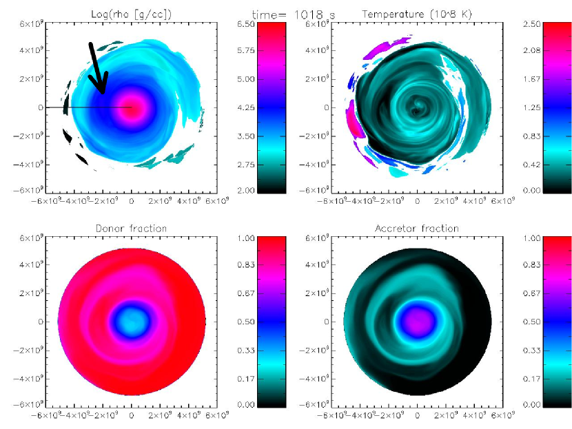
Figure 2: The $q=0.9$ simulation after the two stars have merged showing log density (upper left), temperature (upper right), mass fraction of donor material (lower left), and mass fraction of accretor material (lower right) in the equatorial plane. The horizontal line in the density plot illustrates where the plot in Fig. 3 is made. Much of the donor material is violently digging into the accretor core (density larger than $10^{5.2}{\rm g/cm^{3}}$) during the merger. In the process, accretor material is being dredged up, mixing with the incoming donor material mostly in a layer just outside the core. The central region with a density larger than about $10^{4}{\rm g/cm^{3}}$ can be seen to be somewhat asymmetric. A colder, donor rich “blob” of material sits to the left of the central high density core (around $2\times 10^{9}$ cm from the center), indicated by the arrow in the density plot. This blob is found to be more prominent in the $q=0.7$ simulation.

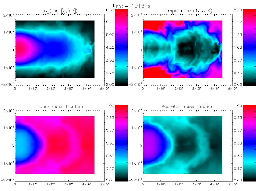
Figure 3: The $q=0.9$ simulation after the two stars have merged, showing log density (upper left), temperature (upper right), mass fraction of donor material (lower left), and mass fraction of accretor material (lower right) in the r-z plane from the center of the grid outwards, intersecting the blob (along the line in the density plot in Fig. 2). Little mass is being forced out in the vertical direction, explaining the very low densities far from the equator.

We now discuss the details of the high and low $q$ simulations, choosing $q=0.9$ and $q=0.7$ as our representative cases. The merger in the high $q$ simulations (Figs. 2 and 3) is extremely violent, and the accretor core is severely distorted by the incoming accretion stream. A thin layer just outside of the combined core contains a mixture of donor and accretor material. Assuming a composition of carbon and oxygen only, the temperature in the high density regions does not reach $10^{8}$ K other than in a few transient areas during and after the merger.

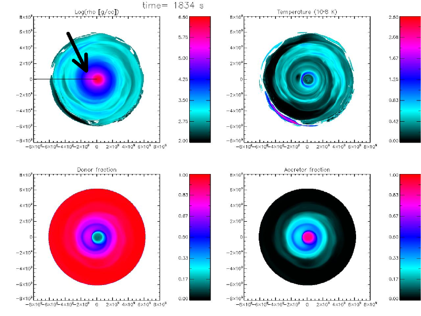
Figure 4: The $q=0.7$ simulation after the two stars have merged, showing log density (upper left), temperature (upper right), mass fraction of donor material (lower left), and mass fraction of accretor material (lower right) in the equatorial (r-$\phi$) plane. The horizontal line in the density plot illustrates where the plot in Fig. 5 is made. Compared to the higher-$q$ simulations, there are noticeable differences in this simulation. A hot SOF forms around the merged core with temperatures up to $1.5\times 10^{8}$ K (assuming C and O only; from Fig. 5 we can see that this is actually a SOF). The merger is also less violent, in that the accretor core is not distorted as much as in the higher $q$ cases. However, much accretor material is being dredged up during the merger. The core is seen to be asymmetric. A cold, donor-rich blob sits to the left of the central, highest density core, indicated by the arrow in the density plot.

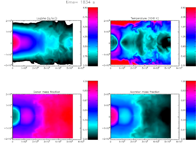
Figure 5: The $q=0.7$ simulation after the two stars have merged, showing log density (upper left), temperature (upper right), mass fraction of donor material (lower left), and mass fraction of accretor material (lower right) in the r-z plane, intersecting the blob (along the line in the density plot in Fig. 4). A hot SOF develops around the merged core, with temperatures up to about $1.5\times 10^{8}$ K (assuming C and O only). Even though the core is not distorted as much as in the higher $q$ simulations, we notice that much accretor and donor material is pushed up vertically from the core. The donor rich blob is clearly visible in the mass fraction plots of donor and accretor material, between about $8\times 10^{8}$ cm and $2\times 10^{9}$ cm. It can also be seen in the density plot.

Lower $q$ simulations (see Fig. 4 and Fig. 5) show a much less violent merger. Even though the accretor core does not get significantly distorted, a large amount of accretor material is being dredged up and mixes with the incoming donor material. Indeed, the donor star is tidally disrupted before the cores merge. This helps to preserve the SOF in these cases, as the donor material is added more gently on top of the accretor, instead of falling through the SOF to mix in with the core as in the high $q$ simulations. On the other hand, in the high $q$ simulations the two cores merge destroying the SOF in the process to form the newly merged core, by mixing the hot pre-merger SOF material with cold donor and accretor core material.

An asymmetric feature in the merged object becomes very clear in the $q=0.7$ simulation; looking at the density plot in Fig. 4, a lower density blob can be seen extending from the core in the negative “x” direction. This blob has a very low temperature, and to be donor rich/accretor poor (as such it can be thought of as some of the last of the donor material, accreted but never heated). It is encapsulated by accretor rich material. This is also clearly visible in Fig. 5, which shows a slice taken directly through the blob. A blob is also present in the other simulations (both high and low $q$), although it appears most prominent in the $q=0.7$ configuration. The SOF has formed between this blob and the merged core, with sustained temperatures of $\sim 1.5\times 10^{8}$ K or more (assuming C and O only) lasting at least for the duration of the $q=0.7$ simulation (similar features are found in the $q=0.5$ and $0.6$ simulations). In the $q=0.6$ simulation, we find sustained temperatures in the SOF of about $2.5\times 10^{8}$ K, while in the $q=0.5$ simulation the sustained temperatures are about $3\times 10^{8}$ K. We find the SOF (in all low $q$ cases) to be located just outside the merged core ($r\sim 10^{9}$ cm), with a thickness of about $1-2\times 10^{8}$ cm (Table 1). We assume the core of the merged object is where $\rho>10^{5.2}{\rm g/cm^{3}}$ and $T<10^{8}{\rm K}$, while the SOF is defined as being $\rho>10^{4.25}{\rm g/cm^{3}}$ and $T>10^{8}{\rm K}$. The core density value was chosen so that it extends out to the SOF. As we will see in the next section, the low $q$ simulations turn out to be the cases relevant to the nucleosynthesis of ${}^{18}\mathrm{O}$. Table 2 lists the details of the cases and their SOFs.

Table 1: Summary of the conditions found in the SOF after the merger. In particular, $q$ is the mass ratio used in the hydrodynamic simulations, $T_{\rm SOF}$ and $\rho_{\rm SOF}$ are representative values of density and temperature in the SOF, $f_{\rm sof,acc}$ represents the fraction of the SOF made of the accretor material and $dR_{\rm SOF}$ refers to the (approximate) width of the SOF.

q	$T_{\rm sof}$ ($10^{6}$ K)	$\rho_{\rm sof}({\rm g/cm^{3}})$	$f_{\rm sof,acc}$	$dR_{SOF}(10^{9})$ cm
0.5	300	$10^{4.5}$	0.67	0.2
0.6	250	$10^{4.5}$	0.54	0.15
0.7	150	$10^{4.7}$	0.50	0.2

Table 2: For the simulations, we list the mass of the accretor WD (CO; $M_{CO}$), the mass of the donor WD (He WD in lower $q$ simulations; $M_{He}$), the mass of the SOF ($M_{\rm SOF}$), the mass that is present outside the merged core and the SOF ($M_{\rm out}$), the time from the beginning of the simulation to the end of the merger ($t_{merge}$), the total time for which the simulation was run $t_{end}$, and the time for which the simulation ran after the merger ($\delta\rm t$ = $t_{end}-t_{merge}$).

$q$	$M_{CO}/M_{\odot}$	$M_{He}/M_{\odot}$	$M_{\rm SOF}/M_{\odot}$	$M_{\rm out}/M_{\odot}$	$t_{merge}(s)$	$t_{end}(s)$	$\delta\rm t(s)$
0.5	0.6	0.30	0.12	0.24	2070	2542	472
0.6	0.56	0.34	0.13	0.26	1150	1500	350
0.7	0.53	0.37	0.10	0.30	1200	1970	570
0.9	0.47	0.43	none	0.34	667	1084	417
0.99	0.45	0.45	none	0.34	698	1137	439

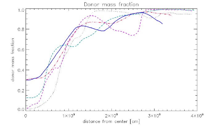
Figure 6: The mass fraction of the donor material as a function of the distance from the center of the merged object at an arbitrary time after merger. The curves are for $q=0.5$ (dotted; black), $q=0.6$ (dashed; purple), $q=0.7$ (dash-dotted; light blue), $q=0.9$ (solid; blue), and $q=0.99$ (dash-triple-dotted; red). The core is about $10^{9}$ cm, surrounded by an SOF for the $q=0.5$, $0.6$, and $0.7$ cases. The mass fraction of the accretor material for each of these cases may be obtained as 1- mass fraction of the donor material.

Table 3: For each of the low-$q$ simulations, the fraction of mass ($f_{\mathrm{acc-dredged}}$) dredged up from the accretor, the accretor mass in the SOF ($m_{\rm acc_{S}OF}/M_{\odot}$) in solar masses and the accretor mass that is outside the SOF ($m_{\rm acc_{o}ut}/M_{\odot}$).

$q$	$f_{\rm acc-dredged}$	$m_{\rm acc-SOF}/M_{\odot}$	$m_{\rm acc_{o}ut}/M_{\odot}$
0.5	0.17	0.08	0.02
0.6	0.18	0.07	0.03
0.7	0.15	0.05	0.03

In Fig. 6, we plot the donor mass fraction as a function of radius in the equatorial plane, where the mass fraction of the accretor material is simply one minus the mass fraction of the donor material. In all simulations (including the low $q$ cases), we find that a significant amount of accretor material is being dredged up and mixed with the donor material outside of the merged core. The dredged up accretor material leads to a layer just outside the core that is heavily enriched with accretor material. Outside the merged core and the SOF, the mass of accretor material is nearly the same in all the low $q$ simulations (Table 3). From Figs. 2 and 3 we see that the high $q$ simulations have considerable mixing in their cores due to the very violent mergers forming them. The low $q$ simulations do not experience such violent mixing.

3.2 R Coronae Borealis progenitor systems

In order to perform nucleosynthesis calculations, we use the temperature and density conditions of the SOFs. Post merger, the SOFs are seen as a feature solely of the low $q$ cases, with temperatures ranging from $1.5\times 10^{8}$ to $3\times 10^{8}$ K (Fig. 1) with densities between ${\rho}=10^{4.25}-10^{5.2}{\rm g/cm^{3}}$ (Table  1). Such conditions make the SOF a favorable site for the production of ${}^{18}\mathrm{O}$ and are used as inputs to the nucleosynthesis code.

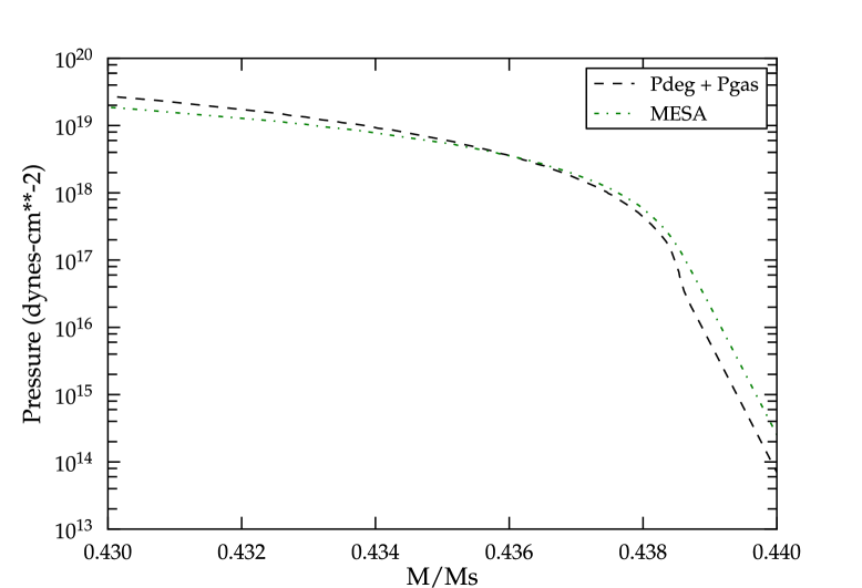
Figure 7: Pressure profile of a model in the 11th thermal pulse on the AGB of an initial mass of 2 $M_{\odot}$, compared against the pressure calculated using the EOS used in the hydrodynamic simulations. The region shown here is typically where the SOF is located during the course of the merger simulations.

Since the SOF is the region where we focus our analysis, we do a simple validation test of the EOS used in the hydrodynamic simulations. To do this, we compare the pressure calculated using this EOS, for the density and temperature of the H-free core of a MESA computed AGB model on its 11th thermal pulse having an initial mass of 2 $M_{\odot}$, against the pressure profile given by MESA for the same model. Fig. 7 shows the outer portion of the CO WD where the SOF appears in the simulations. We can see the pressure of the CO WD model from MESA is very close to that obtained from the EOS used in the hydrodynamic simulations, the pressure being slightly lower within 0.436 $M_{\odot}$ and higher above it. This gives a reasonable confirmation on the choice of the EOS for the purpose of these simulations.

For the nucleosynthesis calculations, the initial chemical abundances in the SOF are required. According to the hydrodynamic simulations, the SOF has contributions from the He WD as well as material dredged up from the CO WD. The initial abundances of the WDs are calculated using realistic 1D stellar evolution models computed with MESA (Paxton et al., 2011) and post processed with NuGrid codes.

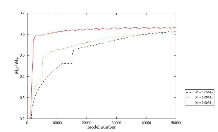
Figure 8: The evolution of the hydrogen free core mass ($M_{H}/M_{\odot}$) during the AGB phase of the star, for three initial masses. The model numbers on the horizontal axis are related to time, with a higher model number being a later time. The AGB thermal pulse phase occurs over a much smaller time period than the previous evolution of the star. Hence, if age were used as the x axis parameter, the thermal pulse features would be compressed and not visible. Model numbers help in visualising the entire range of evolution of the star.

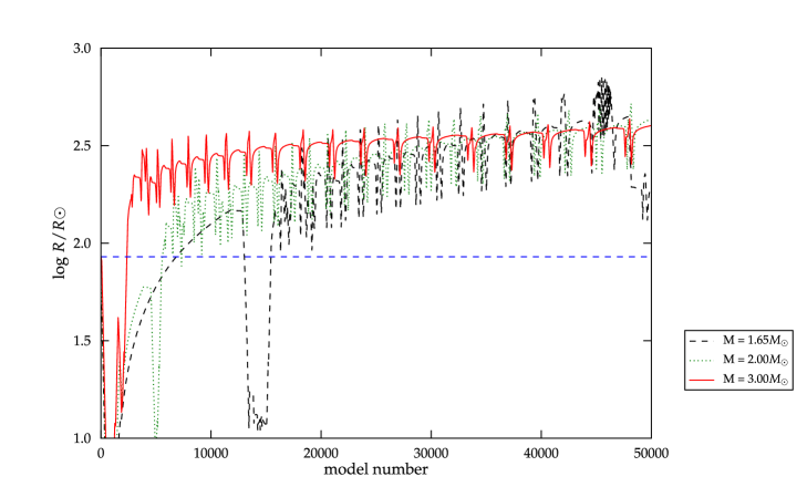
Figure 9: The variation of the radius of the star ($\mathrm{logR/R_{\odot}}$) plotted against the model number, during the AGB phase of the star, for three initial masses. The blue dashed line is the radius of the progenitor RGB star of the He WD under consideration. A model number corresponds to every step in time taken by the code during the run for each initial mass; a higher model number corresponds to at a later point of time.

In order to determine the initial abundance contribution from the CO WD, the evolutionary state of the AGB progenitor from the last common envelope (CE) phase has to be determined. During the likely binary progenitor evolution that leads to the double degenerate merger considered here, one or more CE phases can occur (Iben & Tutukov, 1984). For the scenario that we consider, there are two CE phases. The first one occurs when the primary star overflows its Roche lobe during its AGB phase, thus forming the CO WD. For a star to fill its Roche lobe, its radius must be greater than or equal to its Roche lobe radius ($R_{L}$). $R_{L}$ is the product of a function of the mass ratio $E(q)$ between the primary and the secondary components of the binary system and the separation ($a$) between them, given by $R_{L}=E(q)a$ (Eggleton, 1983). From observations of binary systems, the separation between components can range between $3-10^{4}R_{\odot}$ (Hurley et al., 2002), which implies that the $R_{L}$ of a star in a binary system, with a given initial mass ratio, can vary over 4 orders of magnitude depending on the separation distance between the two components.

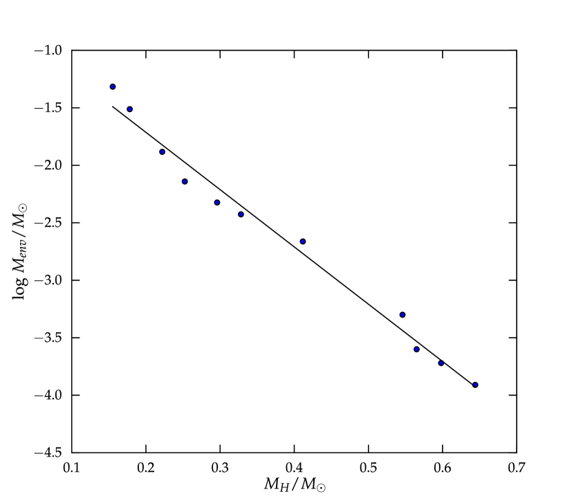
Figure 10: Plot showing the anti-correlation between envelope mass (log $M_{env}/M_{\odot}$ and hydrogen-free core mass $M_{H}/M_{\odot}$. A best fit line using the least squares method is drawn through the blue data points.

From stellar evolution studies, the structure of a WD consists of a hydrogen free core, $M_{H}$, surrounded by a thin envelope of unprocessed material which as a result is rich in hydrogen. The envelope mass is typically between 0.05 to 1$\%$ of the mass of the WD and is anti-correlated with $M_{H}$ where the outer boundary is the radial co-ordinate at which the hydrogen abundance $X_{H}$ = 0.37 (Schönberner, 1983). Using the data from the work of Schönberner (1983) for CO WDs and Driebe et al. (1998) for He WDs, a least squares fit is done between the data points. The best fit line thus constructed enables us to read off the envelope mass, $M_{env}$, for a particular $M_{H}$ (between 0.1552 and 0.644 $M_{\odot}$) (Fig. 10). The analytic equation of this line is $\log(M_{env}/M_{\odot})=-4.982M_{H}/M_{\odot}-0.7171$ .

The hydrodynamic simulations of interest for nucleosynthesis, use a range of masses of CO WDs ($M_{CO}$) between 0.53 and 0.6 $M_{\odot}$. For the purposes of the following explanation, we can take $M_{CO}=M_{H}$ since the envelope mass ($M_{env}$) of the CO WD is less than $0.1\%$ of its total mass.

However, knowing the white dwarf mass does not imply knowledge of the initial mass of its progenitor star. Figure 8 shows the evolution of $M_{H}$ (${\sim}M_{WD}$) (NuGrid Set1.2 models for solar metallicity, Pignatari et al. 2012, in preparation) for a range of stellar masses ($1.65,2$ and $3M_{\odot}$). It is evident that for a given value of $M_{H}$ the star could have any of the three initial masses and can lie anywhere between the early AGB phase and a late thermal pulsing (TP) phase. The higher the number of TPs that the star has undergone, the more enriched it is in partial He-burning and s-process products (Herwig, 2005). A parameter that will help in solving this degeneracy between the initial and the core mass of a star is the Roche lobe radius of the giant star that first fills its Roche lobe in the binary system. Fig. 9 shows the radius evolution of the AGB stellar model sequences for the same initial masses.

Let us consider an He WD model from the cases plotted, whose mass is nearly the same as the one in the $q=0.5$ simulation. This model has mass $M_{He}=0.3024M_{\odot}$ from a star of initial mass of 1.65 $M_{\odot}$. If we assume that the RGB progenitor of this He WD fills its Roche lobe when it reaches this radius and that the binary system enters its second CE phase immediately when it does so, then it is a good estimate that the maximum separation distance between the two components is at the most, the Roche lobe radius ($\mathrm{log~{}R_{L}/R_{\odot}}$) of the secondary, which is 1.286 in this case.

From previous hydrodynamic simulation work done by De Marco et al. (2011), we know that after the binary system has undergone its first CE event, the separation between the components reduces by at least 4.5 times its initial separation. The minimum separation at the time of the first CE event is at least $\mathrm{log~{}a/R_{\odot}}$ = 1.93. We assume that the binary system enters its first CE phase immediately when the AGB star fills its Roche lobe. Since ($\mathrm{log~{}a/R_{\odot}}$) = 1.93 is the minimum limit on the Roche lobe radius of the AGB star, we investigate three cases during different phases of the AGB star, when its radius exceeds this value. These are, during the early AGB phase (CO WD(1)), an early TP phase (CO WD(2)), and a late TP phase (CO WD(3)) (after the star becomes carbon rich) (Fig. 9). It must be pointed out that the post CE WD abundance profile is assumed to be that of the inner portion of the progenitor AGB models considered here. Henceforth the CO WD models are to be understood as the progenitor AGB stars with mass equal to $M_{CO}=M_{H}$ + $M_{env}$.

Table  4 summarizes the relevant parameters of these CO WD models. It must be noted that while the star is in the TP phase the chosen model must be at the peak of the pulse, since the radius of the star is at its maximum during the peak of a given pulse. If the star has not been able to fill its Roche lobe during an earlier pulse peak, it cannot do so until it hits the next pulse peak.

From the hydrodynamic simulations it is seen that the He WD is totally disrupted and well mixed during the final merging phase. Hence for the He WD the nuclear abundances are averaged over its entire mass, thus giving a uniform composition for the He WD. From Table  3, the fraction of CO WD dredged up outside is less than $20\%$. Table  5 contains the isotopic abundances of the He WD and the cumulative abundances of significant elements in the outer $20\%$ of the CO WD models.

In order to achieve an extremely low ${}^{16}\mathrm{O}/^{18}\mathrm{O}$ ratio such as that observed in RCB stars, we take the CO WD model which provides the abundances most viable to help realize this. The model which has the highest amount of ${}^{14}\mathrm{N}$ and ${}^{18}\mathrm{O}$ and the least amount of ${}^{16}\mathrm{O}$, amongst the three cases is selected. This model belongs to the early AGB phase of the 3 $M_{\odot}$ star , (Fig. 11) and has $M_{CO}$=0.58148 $M_{\odot}$ (CO WD(1), Table  4) and an envelope of $2.5\times 10^{-4}M_{\odot}$. It must be noted that since the progenitor of the CO WD model chosen is on the E-AGB, it does not have any s-process element enhancement on it’s surface. Hence although the choice of this CO WD model may lead to the reproduction of the unique O isotopic ratio values of RCB stars, it may not reproduce the s-process element enrichment found in them.

Thus we have used the CO WD and He WD models described above, to provide the initial abundances of the SOF. With the knowledge of the the fraction of the SOF made of the accretor ($f_{\rm sof,acc}$) and the donor (1-$f_{\rm sof,acc}$, Table 1), the initial abundances of the SOF are constructed (Table  6). We assume that all the material from the CO WD has been dredged up from its outer layers, before the onset of hot nucleosynthesis in the SOF.

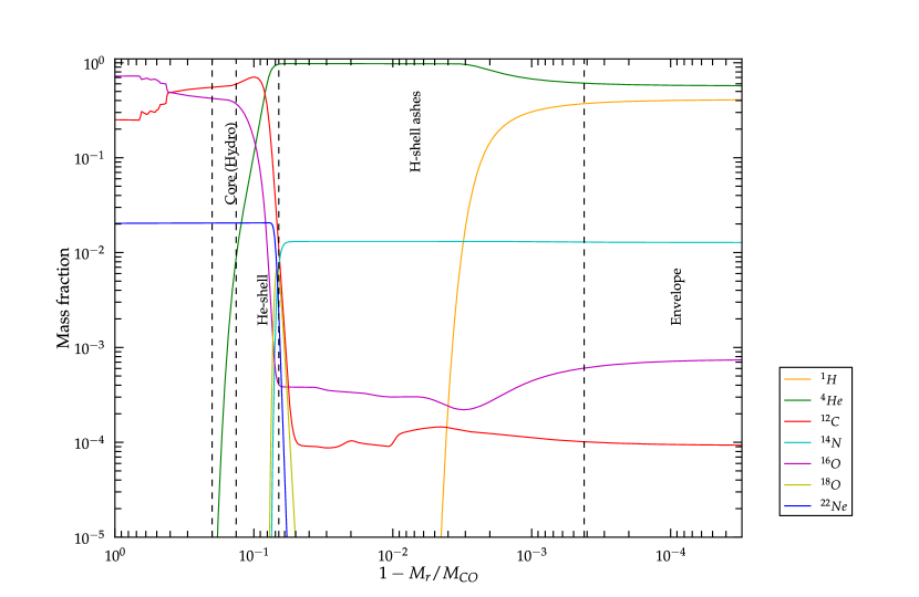
Figure 11: Nuclear abundance profile of the CO WD (1) model. The x-axis is $(1-M_{r}/M_{CO})$ where $M_{r}$ is the radial mass co-ordinate and $M_{CO}$ = 0.58148. The zones of the CO WD are labelled and marked with dashed black lines. The lower limit on the zone marked “Core (hydro)” is placed at a depth enclosing $20\%$ of the $M_{CO}$ mass, which is the upper limit on the mass dredged up of the CO WD as seen in the hydrodynamic simulations.

Table 4: The details of the CO WD models - initial mass ($M_{\star}$), model number, phase of evolution, mass of the CO WD ($M_{CO}/M_{\odot}$), mass of hydrogen free core ($M_{H}/M_{\odot}$), and $\mathrm{log~{}R/R_{\odot}}$.

Serial number	$M_{\star}$	model number	phase of evolution	$M_{H}/M_{\odot}$	$M_{CO}/M_{\odot}$	$\mathrm{log~{}R/R_{\odot}}$
1	3	2364	E-AGB	0.58123	0.58148	1.97
2	2	12198	3$\mathrm{rd}$ TP	0.53334	0.53376	2.35
3	2	49901	21$\mathrm{st}$ TP	0.61226	0.612243	2.65

Table 5: The averaged (approximate) abundances ($\%$) by mass, for dominant and relevant species for the evolution of the abundance of ${}^{18}\mathrm{O}$ in the outer part of the three CO WDs are presented in Table 4 (we considered the most external zone, which corresponds to about $20\%$ of the total WD masses). The other nearly 300 species in the nuclear network of the code, are present in much smaller proportions.

Species	He WD	CO WD (1)	CO WD (2)	CO WD (3)
${}^{1}\mathrm{H}$	1.51	0.33	0.276	0.093
${}^{4}\mathrm{He}$	96.5	41.7	14.6	9.04
${}^{12}\mathrm{C}$	0.011	36.5	50.5	43.9
${}^{14}\mathrm{N}$	1.3	0.43	0.061	0.155
${}^{16}\mathrm{O}$	0.074	19.0	32.0	43.8
${}^{18}\mathrm{O}$	2.86${\times}10^{-5}$	2.7${\times}10^{-3}$	2.71${\times}10^{-4}$	1.11${\times}10^{-5}$
${}^{22}\mathrm{Ne}$	2.73${\times}10^{-4}$	1.34	1.95	2.18

Table 6: The averaged initial abundances ($\%$) for dominant and relevant species for the evolution of the abundance of ${}^{18}\mathrm{O}$ in the SOF of the $q=0.5$, $0.6$, and $0.7$ cases using the He WD and CO WD(1) models of Table 5. The other nearly 300 species in the nuclear network of the code, are present in much smaller proportions.

Species	SOF,0.5	SOF,0.6	SOF,0.7
${}^{1}\mathrm{H}$	0.75	0.89	0.97
${}^{4}\mathrm{He}$	64.8	69.5	75.9
${}^{12}\mathrm{C}$	22.2	18.6	15.1
${}^{14}\mathrm{N}$	0.76	0.85	0.92
${}^{16}\mathrm{O}$	10.03	8.9	5.9
${}^{18}\mathrm{O}$	0.021	0.016	0.018
${}^{22}\mathrm{Ne}$	0.81	0.68	0.55

3.3 Nucleosynthesis

The SOF is present until the end of the simulations for all three low-$q$ cases, hence it is not known for how long the conditions in the SOF would last. Therefore, we run the nucleosynthesis simulation until the abundance of ${}^{18}\mathrm{O}$ begins to drop significantly. The ${}^{18}\mathrm{O}$ abundance drops to $10^{-8}$ at $\sim 10^{7}$ seconds from the beginning of the nucleosynthesis run. We take this time period for the other two low-q cases as well and run the nucleosynthesis network at the chosen constant temperature and density (Table  1). In order to compare with observations, the abundances of all unstable elements are instantaneously decayed. These abundances are plotted in Figs. 12, 13, and 14, for $q=0.5$, $0.6$, and $0.7$. Since the densities in the SOF are similar amongst the low-$q$ cases, the differences in the final chemical abundances arise mainly due to the different temperatures. Hence in order to understand the role of nuclear processes for different species, we take the case that showcases them over the shortest amount of time, viz., the $q=0.5$ case.

In Fig. 12, it is seen that between $10^{-3}$ and $10^{-1}$ seconds, proton capture reactions on ${}^{12}\mathrm{C}$, ${}^{14}\mathrm{N}$, ${}^{18}\mathrm{O}$ and ${}^{19}\mathrm{F}$ bring down their initial abundances by an order of 1.5 to 3. Compared to the initial abundance, the ${}^{18}\mathrm{O}$ abundance drops several orders of magnitude in $10^{-2}$ seconds. This implies that the amount of initial ${}^{18}\mathrm{O}$ abundance does not help much in lowering the ${}^{16}\mathrm{O}/^{18}\mathrm{O}$ ratio since most of the ${}^{18}\mathrm{O}$ present initially is destroyed. The ${}^{13}\mathrm{N}$ abundance reaches a quasi equilibrium value of 0.1 after 0.2 seconds via the destruction of ${}^{12}\mathrm{C}$ by ${}^{12}\mathrm{C(p,\gamma)}^{13}\mathrm{N}$. Since the plotted abundances are only of stable nuclei, the rise in ${}^{13}\mathrm{N}$ abundance is reflected in the increase of ${}^{13}\mathrm{C}$.

From $10^{-1}$ to $10^{3}$ seconds, the above nuclei are regenerated by the same proton capture reactions that caused their destruction earlier, viz.,

$${}^{17}\mathrm{O(p,\gamma)}^{18}\mathrm{F(^{+}\beta)}^{18}\mathrm{O}$$

$${}^{18}\mathrm{O(p,\gamma)}^{19}\mathrm{F}$$ (10)

$${}^{19}\mathrm{F(p,\gamma)}^{20}\mathrm{Ne}$$

During this time, the neutron abundance continually increases. The main source of neutrons is the ${}^{13}\mathrm{C(\alpha,n)}^{16}\mathrm{O}$ reaction, along with ${}^{22}\mathrm{Ne(\alpha,n)}^{25}\mathrm{Mg}$ and other auxillary $(\alpha,n)$ reactions. At $\sim$ 7 seconds, there is a rise in the proton abundance. The three main sources identified to cause an increase of 90$\%$ in the proton abundance are,

$${}^{15}\mathrm{O(n,p)}^{15}\mathrm{N}$$

$${}^{14}\mathrm{N(n,p)}^{14}\mathrm{C}$$ (11)

$${}^{13}\mathrm{N(n,p)}^{13}\mathrm{C}$$

along with smaller contributions from auxillary (n,p) reactions.

The proton abundance begins to drop again at nearly 500 seconds as the rapid consumption overwhelms the production. At 1000 seconds, $\alpha$ capture on ${}^{13}\mathrm{C}$ becomes extremely efficient and its abundance drops rapidly.

The neutron abundance reaches a peak at 2860 seconds and then drops quickly due to consumed by neutron capture reactions. The protons are unable to increase their abundance as the neutron and ${}^{14}\mathrm{O}$ abundance drop to very low values. At the same time that the proton abundance drops, the ${}^{18}\mathrm{O}$ abundance drops suddenly due to ${}^{18}\mathrm{O(p,\gamma)}^{19}\mathrm{F}$ and there is a simultaneous increase in the ${}^{19}\mathrm{F}$ abundance.

Thereafter, it is the reign of partial helium burning reactions. Beginning from 3000 seconds, the abundance of ${}^{16}\mathrm{O}$,${}^{18}\mathrm{O}$ and ${}^{19}\mathrm{F}$ increase via :

$${}^{12}\mathrm{C(\alpha,\gamma)}^{16}\mathrm{O}$$

$${}^{14}\mathrm{N(\alpha,\gamma)}^{18}\mathrm{F(\beta^{+})}^{18}\mathrm{O}$$ (12)

$${}^{15}\mathrm{N(\alpha,\gamma)}^{19}\mathrm{F}$$

At around 40,000 seconds ${}^{18}\mathrm{O}$ reaches its peak and begins to be converted to ${}^{22}\mathrm{Ne}$ by ${}^{18}\mathrm{O(\alpha,\gamma)}^{22}\mathrm{Ne}$. This destruction exceeds the production of ${}^{18}\mathrm{O}$ and its abundance drops to $10^{-8}$ at $10^{8}$ seconds and continues to drop as time goes on.

The $q=0.6$ and $0.7$ cases with a constant temperature of $T=1.23\times 10^{8}K$ and $T=2.1\times 10^{8}K$ (these temperatures are calculated assuming the abundances given in Table 6), respectively, show a much slower evolution of nuclear abundances (Figs. 13, and 14) compared to the $q=0.5$ case. Over a longer time period, these cases will also show the same abundance trends as the $q=0.5$ case.

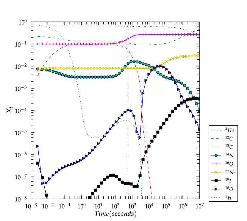
Figure 12: Evolution of the nuclear species when starting with conditions similar to those found in the SOF in the $q=0.5$ simulation with $T=2.4\times 10^{8}K$ and $\rho=10^{4.5}$ over a period of $10^{6}$ seconds. The hydrogen abundance is multiplied by a factor of $10^{2}$. The dashed vertical line corresponds to $\delta\rm t$ (Table 2).

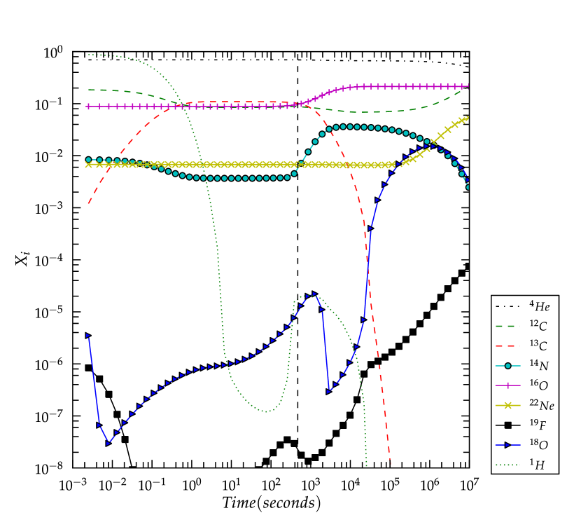
Figure 13: Evolution of the nuclear species when starting with conditions similar to those found in the SOF in the $q=0.6$ simulation at $T=2.1\times 10^{8}$ K and $\rho=10^{4.5}{\rm g/cm^{3}}$ over a period of $10^{6}$ seconds. The hydrogen abundance is multiplied by a factor of $10^{2}$. The dashed vertical line corresponds to $\delta\rm t$ (Table 2).

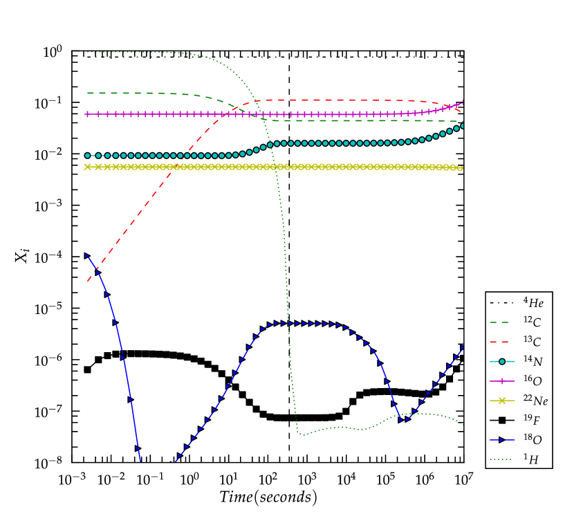
Figure 14: Evolution of the nuclear species when starting with conditions similar to those found in the SOF in the $q=0.7$ simulation at $T=1.23\times 10^{8}$ K and $\rho=10^{4.7}{\rm g/cm^{3}}$ over a period of $10^{6}$ seconds. The hydrogen abundance is multiplied by a factor of $10^{2}$. The dashed vertical line corresponds to $\delta\rm t$ (Table 2).

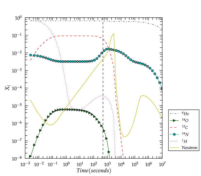
Figure 15: Evolution of the neutron abundance in the SOF of the $q=0.5$ simulation, along with those species relevant to its evolution. The dashed vertical line corresponds to $\delta\rm t$ (Table 2). The neutron abundance is multiplied by a factor of $10^{13}$.

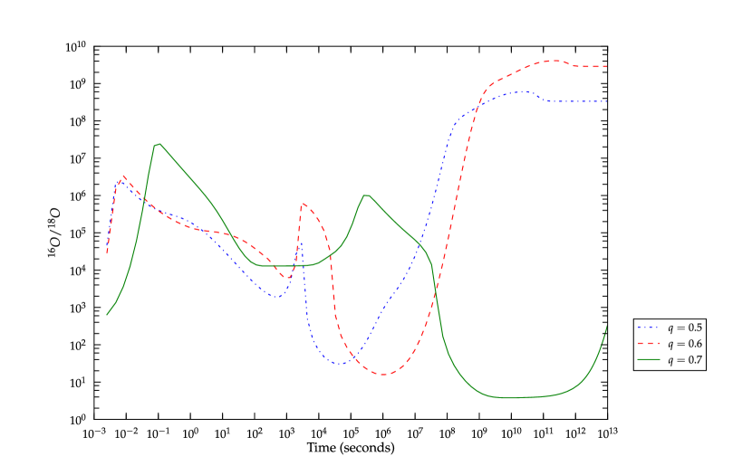
Figure 16: Evolution of the ${}^{16}\mathrm{O}/^{18}\mathrm{O}$ ratio in the SOF of the $q=0.5$, $0.6$, and $0.7$ cases from $10^{-3}$ to $10^{13}$ seconds.

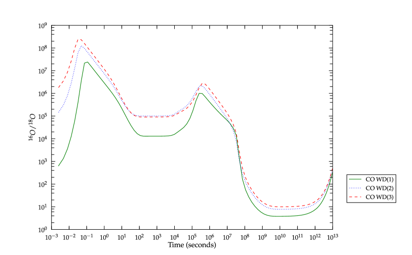
Figure 17: Evolution of the ${}^{16}\mathrm{O}/^{18}\mathrm{O}$ ratio for initial abundances build from CO WD (1),(2) and (3) in Table 4 for the SOF of the $q=0.7$ case between $10^{-3}$ and $10^{13}$ seconds.

Fig. 16 plots the evolution of ${}^{16}\mathrm{O}/^{18}\mathrm{O}$ in the SOF for each low-q case. To construct this plot the nucleosynthesis network was run for a longer time period viz., $10^{13}$ seconds. Within the time scale of the plots in Figs. 12,  13, and  14 the lowest ${}^{16}\mathrm{O}/^{18}\mathrm{O}$ value in the SOF is $\sim$ 16 and is found in the $q=0.6$ case at about $10^{6}$ seconds after the SOF forms. It increases to 23 in $2.4{\times}10^{6}$ seconds and continues to increase thereon. In the $q=0.5$ case, the minimum value of this ratio is $\sim$ 30, which is higher than the 0.6 case due to a faster destruction of ${}^{18}\mathrm{O}$ to ${}^{22}\mathrm{Ne}$ while in the 0.7 case the minimum value is ${\sim}$ 13,900 as there is hardly any ${}^{18}\mathrm{O}$ being produced.

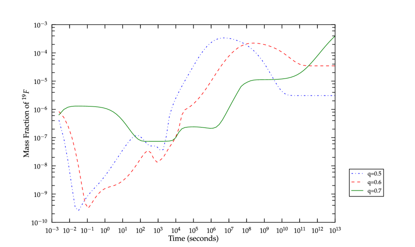
Figure 18: Evolution of the ${}^{19}\mathrm{F}$ mass fraction in the SOF of the $q=0.5$, $0.6$, and $0.7$ cases from $10^{-3}$ to $10^{13}$ seconds.

Certain RCB stars are observed to be enriched in ${}^{19}\mathrm{F}$ on their surface indicating an overabundance of ${}^{18}\mathrm{O}$, however ${}^{18}\mathrm{O}$ and ${}^{19}\mathrm{F}$ are not measured in the same stars. The range of observed ${}^{19}\mathrm{F}$ abundances in the RCB majority stars is between $7.5\times 10^{-6}$ to $3\times 10^{-4}$ (Pandey et al., 2008). During the course of the long term evolution of the $q=0.5$ case, the ${}^{15}\mathrm{N(\alpha,\gamma)}^{19}\mathrm{F}$ reaction generates a high amount of ${}^{19}\mathrm{F}$ and comes to an equilibrium value after $10^{10}$ seconds. This amount falls within the range of the observed ${}^{19}\mathrm{F}$ abundances of the majority of RCB stars for all three low-q cases (Fig. 18). The $q=0.5$ and $0.6$ simulations show peaks in the ${}^{19}\mathrm{F}$ abundance between $10^{5}$ and $10^{9}$ seconds. Interestingly, the oxygen ratio is at a minimum of 16 at $10^{6}$ seconds for $q=0.6$ (Fig. 16, making it possible to have a low oxygen ratio at the same time as ${}^{19}\mathrm{F}$ is enhanced.

However on maintaining the temperature, density conditions of the 0.7 case for $10^{10}$ seconds, the lowest possible ${}^{16}\mathrm{O}/^{18}\mathrm{O}$ value in the SOF is found to be $\sim 4$. The oxygen isotopic ratio stays close to 5 between $10^{9}$ and $10^{12}$ seconds. Thus, it is possible to reproduce in the SOF the ${}^{16}\mathrm{O}/^{18}\mathrm{O}$ ratio found in RCB stars for a significantly large period of time. However, it requires the initial abundances of the SOF of the 0.7 case and the sustenance of constant temperature and density conditions of this case.

We recall that the maximum amount of ${}^{18}\mathrm{O}$ that can be produced is also limited by the amount of ${}^{14}\mathrm{N}$ present. The metallicity of the He WD progenitor determines the initial abundance of ${}^{14}\mathrm{N}$ but as can be seen in the nucleosynthesis calculations, new ${}^{14}\mathrm{N}$ is formed by H-burning via the partial CNO cycle. The dredge up of accretor material and consequently the ${}^{16}\mathrm{O}$ added to the SOF poses another constraint on this oxygen isotopic ratio.

In order to confirm that this is the lowest ${}^{16}\mathrm{O}/^{18}\mathrm{O}$ value one can get from our grid of CO WD models (Sec. 3.2), the nucleosynthesis calculations are also done by constructing initial abundances in the same manner as done for the SOF of the $q=0.7$ case by using the same He WD model and the other CO WD models, CO WD(2) and (3). The evolution of the isotopic ratio for these cases is shown in Fig. 17 and it can be seen that indeed the lowest value is found for the progenitor system containing model CO WD (1).

In order to estimate an approximate value of this ratio in the surface of the merged object, we mix the post nucleosynthesis material of the SOF with the layer above it. The surface is defined as the SOF plus the layer on top of it. For the purpose of a rough estimate, we assume that the material above the SOF has not undergone nucleosynthesis but just contains a proportion of He and CO WD material according to Table 3. For every timestep of the nucleosynthesis calculation of the SOFs of all three low-q cases (as in Fig. 16), we mix the abundances of ${}^{16}\mathrm{O}$ and ${}^{18}\mathrm{O}$ with those in the unprocessed layer above it. The lowest value of ${}^{16}\mathrm{O}/^{18}\mathrm{O}$ amongst all three cases thus obtained in the surface, is 4.6 (corresponding to the same timestep at which 4 is obtained) belonging to the $q=0.7$ case.

The above results are from single zone nucleosynthesis calculations. It would be important to perform multi-zone calculations as well in order to consider the role of mixing between different layers of the star and its consequences for the abundances.

From the nucleosynthesis calculations for each $q$, we also compute the total energy released by nuclear processes per unit time in the SOF (Fig. 19). Note that the energy calculated here does not account for the loss of energy by neutrinos from weak interactions and therefore the energy added to the SOF will be lower by a factor of 1.5-2. Taking this into account, we see from (Fig. 19) that within the timescale of the simulation ($\delta\rm t$ in Table 2) the nuclear energy released is comparable to the internal energy of the SOF (depending on the initial $q$). The energy released in the first few hundred seconds is mainly from proton captures. Helium (for instance, triple $\alpha$ or ${}^{14}\mathrm{N}(\alpha,\gamma)^{18}\mathrm{F}$) interacts on a much longer timescale resulting in a plateau for $q=0.5$ and $0.6$ in Fig. 19 between 10 and 100 seconds. The extra energy released from nuclear processes may lead to higher temperatures, and these processes could play an important role in determining the temperature of the SOF. Cooling processes and dynamical effects may also be important but these cannot be estimated with our current tools.

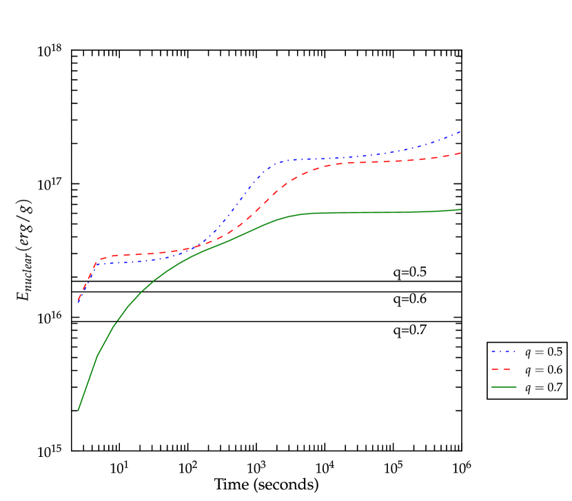
Figure 19: The cumulative energy via nuclear processes released as a function of time for the three cases. We note that these are upper limits on how much energy would be added to the SOF, since energy lost by neutrinos are not taken into account, and hence may be higher by a factor of 1.5-2. The solid horizontal black lines indicate the internal energy in the SOF at the end of the simulation.

4 Comparison to recent WD merger simulations

Our nucleosynthesis calculations were made assuming constant temperature and density. In the SOF, the temperature in the hydrodynamics simulations are found to fluctuate significantly, especially during the actual merger where the temperature may briefly reach up towards $3.5\times 10^{8}$ K (assuming C and O only). Also, the SOF spans a range of densities, something that our nucleosynthesis calculations cannot capture. More elaborate nucleosynthesis calculations (preferably included in the hydrodynamics simulations) should be performed in order to find accurate abundance ratios. The simulation discussed in Longland et al. (2011) does include a (simple) nucleosynthesis network in the dynamics calculations followed by a more elaborate nucleosynthesis calculation in the post processing, and they find ${}^{16}\mathrm{O}$ to ${}^{18}\mathrm{O}$ ratios similar to this study.

The oxygen isotopic ratio is $\sim 1200$ in the $q=0.5$ simulation reported here after 1000 seconds (the dynamical time scale), and is much higher than the lowest value of 19 reported for $q=0.5$ in Longland et al. (2011), and about the same as their ratio of 370 for a fully convective envelope. The total mass in that simulation is higher than the total mass used in our simulations which will affect the temperatures and maybe also the dredge-up, possibly explaining the differences between their results and ours.

Raskin et al. (2012) also presented simulations of WD mergers with higher total masses (their focus was on type Ia supernovae). A noticeable difference between their findings and ours is that they have an “SOF” (or at least a hot ring surrounding their merged core; the 3D temperature structure is not shown in the paper) even in the equal mass simulations. We only find a post merger SOF for $q\lesssim 0.7$. The merged core in the equal mass ($q=1$) simulations in Raskin et al. (2012) appears to be cold, indicating that there has not been much mixing occurring in the core (however in their $0.64M_{\odot}\times 2$ simulation the cores appear to mix similarly to our findings; this is also their simulation that is closest to ours in mass). The SPH simulations of Longland et al. (2011) and Raskin et al. (2012) are not only for a different total mass, but also include nucleosynthesis, and it is plausible that it can cause the differences between their results and ours, especially the fairly rapid burning of the helium atmosphere of their WDs. Our hydrodynamics simulations did not include the energy released from nuclear processes. We showed that this energy is comparable to the thermal energy in the SOF. In the short period of time that the hydrodynamics simulations ran, this extra energy input will probably not make much of a difference. However, on a longer time scale, with even more energy input from nuclear reactions, it is possible that the conditions in the SOF will not remain constant as we assumed in Fig. 16. However, a higher thermal energy can also make the SOF expand. Following the dynamics for a much longer time, including the energy produced in nuclear processes, is needed in order to fully understand the evolution of the SOF.

5 Discussion

The ratio of ${}^{16}{\mathrm{O}}$ to ${}^{18}{\mathrm{O}}$ is observed to be very low (of the order unity) in RCB stars. From hydrodynamic simulations of double degenerate mergers for various mass ratios, we have therefore looked for conditions that would allow for production of ${}^{18}{\mathrm{O}}$ in order to explain this ratio. This requires temperatures of the order $\sim 1.5$ - $3\times 10^{8}$ K. At lower temperatures, ${}^{18}{\mathrm{O}}$ will not form on the available dynamic time scale, and at higher temperatures it will be destroyed (converted to ${}^{22}\mathrm{Ne}$) as soon as it forms. Our results show that the maximum temperature that can be found in the SOF depends strongly on the mass ratio, $q$. Low values of $q$ give temperatures in the SOF of $1.2-2.5\times 10^{8}$ K (assuming realistic abundances), while mass ratios above $q=0.7$ gives temperatures much lower than that. Hence the lower $q$ values that we have investigated will give temperatures in the SOF suitable for ${}^{18}{\mathrm{O}}$ production on a dynamical timescale.

On a dynamical time scale, we do not find very low oxygen ratios in the SOF in any of our simulations. After a thousand seconds, the $q=0.5$ simulation reaches a ${}^{16}\mathrm{O}$ to ${}^{18}\mathrm{O}$ ratio of about 2000, since not much ${}^{18}\mathrm{O}$ is produced on such a short time scale and because of the large amount of ${}^{16}\mathrm{O}$ present from the dredge up. Within a day, the oxygen ratio in the $q=0.5$ simulation reaches its lowest value of $\sim 30$ (Fig. 16). After that, ${}^{18}\mathrm{O}$ is being destroyed and the ratio increases. The $q=0.6$ simulation reaches its lowest value of 16 after $10^{6}-10^{7}$ seconds, after which the ratio increases again as ${}^{18}\mathrm{O}$ is being destroyed. The best case for obtaining low oxygen ratios is the $q=0.7$ simulation, which reaches the lowest ${}^{16}\mathrm{O}$ to ${}^{18}\mathrm{O}$ of $4$ after $\sim 10^{2}$ years, assuming the conditions remain constant for that long. This is comparable to the observed oxygen ratios in RCB stars. As we have shown, the nuclear reactions begin very fast, and the extra energy released is likely to affect the conditions in the SOF. Unfortunately we cannot model this at present, and here we simply state that if the very low oxygen ratios of order unity shall be achieved in the $q=0.7$ simulations, the conditions in the SOF must remain relatively unchanged for a period of about a hundred years.

In the high-$q$ simulations the temperature was not sufficiently high to produce ${}^{18}\mathrm{O}$. However, as we have shown the protons react very quickly, releasing an amount of energy comparable to the thermal energy in the SOF. Hence, it is possible that even in the high $q$ simulations, the SOF prior to the merger can become sufficiently hot for the nucleosynthesis involving helium to start. This extra energy from nuclear processes leads to an extra pressure term, that could potentially help preserve the SOF also in the high-$q$ simulations so that the ${}^{18}\mathrm{O}$ production can continue. Furthermore, even though the amount of ${}^{18}\mathrm{O}$ in RCBs is strongly enhanced compared to all other known objects, it is important to keep in mind that among RCB stars the observed oxygen ratio varies by 2 orders of magnitude from star to star.

The ${}^{16}{\mathrm{O}}$ to ${}^{18}{\mathrm{O}}$ ratio depends both on the formation of ${}^{18}{\mathrm{O}}$, and also on the amount of ${}^{16}{\mathrm{O}}$ present. In all of our simulations, we have found significant dredge up of accretor material which consists primarily of ${}^{16}{\mathrm{O}}$ and ${}^{12}{\mathrm{C}}$. ${}^{18}{\mathrm{O}}$ is formed from ${}^{14}{\mathrm{N}}$, which in part depends on the initial metallicity of the progenitor stars, assumed to be solar giving about $1\%$ of ${}^{14}{\mathrm{N}}$. But ${}^{14}\mathrm{N}$ is also being produced (Figs. 12, 13, and 14) in the nuclear processes occurring in the SOF. The ${}^{16}\mathrm{O}$ to ${}^{18}\mathrm{O}$ ratios, that we find in the SOF (shown in Figs. 16), are the lowest values possible from our simulations.

If less ${}^{16}\mathrm{O}$ were dredged up from the accretor, then less ${}^{18}\mathrm{O}$ would need to be produced in order to obtain low oxygen ratios. One way to avoid contaminating the SOF with ${}^{16}\mathrm{O}$ from dredge-up, would be if the accretor is a hybrid He/CO WD. Rappaport et al. (2009) modeled a $0.475M_{\odot}$ hybrid He/CO WD with a He envelope of more than $0.1M_{\odot}$. In our simulations, we found that about $0.1M_{\odot}$ of accretor material was dredged-up, most of it ending up in the SOF. If the accretor is a hybrid He/CO WD, most of this dredged-up material might turn out to be ${}^{4}\mathrm{He}$, and the ${}^{16}\mathrm{O}$ contamination of the SOF would be much less. In this case, the lower mass of the accretor means the donor must also have a lower mass in order to get a tidal disruption of the donor rather than a core merging. This lower total mass could result in lower temperatures. Furthermore, a mixture with mostly He could also lead to lower temperatures (Eqs. 8 and 9). However, as we discussed above, the reacting protons might heat the gas to a sufficiently high temperature to start the helium burning no matter what the total mass. Hence, it remains to be seen if the oxygen isotope ratio will be of the correct order if this is the situation. Han et al. (2002, 2003) showed that a significant fraction of sdB stars are expected to be in close-period binaries with He WDs. After completion of helium burning, sdB stars may evolve into hybrid CO/He WDs (Justham et al., 2011). In Clausen et al. (2012), a population synthesis study found that there should be almost 200,000 sdB stars in binaries in the galaxy. Hence it may not be unreasonable that a small fraction of these are in a close binary with a He WD, and that after the sdB star has evolved into a hybrid WD they can merge.

When the merged object begins to expand, the temperature and density of the SOF are likely to drop which may bring the nuclear processes there to a halt. Hence the oxygen ratio in the SOF at that time may be representative of what will be observed at the surface of this object. With our numerical approach, we cannot determine when the merged object will begin to expand.

Convection may be triggered quickly in the SOF, as the thermal diffusion time ($\tau_{\rm th}\sim 10^{9}$ seconds using $\varepsilon_{\rm th}\sim 10^{7}{\rm~{}erg~{}g^{-1}~{}s^{-1}}$ from Yoon et al., 2007) is much larger than the 100 seconds thermonuclear time scale ($\tau_{\rm nuc}=c_{p}T/\epsilon_{\rm nuc}$, where $c_{p}$ is the specific heat at constant pressure that we estimate to be of order $10^{8}$ erg/g K, $T$ is the temperature of order $10^{8}$ K, and $\epsilon_{\rm nuc}$ is the nuclear energy production rate of order $10^{14}{\rm~{}erg~{}g^{-1}~{}s^{-1}}$ after 1000 seconds; Fig.19).

If the material outside the merged core and the SOF accretes quickly, it could affect the SOF. Shen et al. (2012) argued that the viscous time scale for material in a disk surrounding such a core is an hour to a year, indicating that it could accrete relatively fast. Alternatively, the merged object can expand before this material has accreted. In that case, the SOF is unlikely to be affected much by this material. However, the Shen et al. (2012) result would indicate that the expansion would have to begin quickly (less than a year) since the accretion may occur on this time scale. We found in the $q=0.6$ simulation that the oxygen ratio is 16 after only $10^{6}$ seconds, a significant enhancement from the solar value and comparable to what is seen in some RCBs.

We note that most of the accretor material, that is being dredged up, ends up in the SOF. The material outside the SOF is mostly from the He WD (Table 3). The conditions outside the SOF are not favorable for nuclear processes to occur, and so if only the matter outside the SOF swells up to supergiant size (without mixing in newly produced elements in the SOF), the resulting object could look like a helium star with some carbon, ie. an RCB star.

We have found that the best conditions for reaching the low oxygen ratios occur if the temperature remains $\sim 10^{8}$ K. Then ${}^{18}\mathrm{O}$ forms slowly, and is destroyed even more slowly. Hence it is plausible that the merger of a CO WD and a He WD can lead to the formation of an RCB star, although a more elaborate investigation must be performed in order to conclusively answer this question.

References

- Asplund et al. (2000) Asplund, M., Gustafsson, B., Lambert, D. L., & Rao N. K. 2000, A&A, 353, 287
- Benz et al. (1990) Benz, W., Cameron, A. G. W., Press, W. H., & Bowers, R.L. 1990, ApJ, 348,647
- Brown et al. (2011) Brown, W. R., Kilic, M, Hermes, J. J., Prieto, C. A., Kenyon, S. J, & Winget, D. E., 2011, ApJL, 737, 23
- Chandrasekhar (1939) Chandrasekhar, S. 1939, An introduction to the Study of Stellar Structure (Chicago, IL: Univ. Chicago Press)
- Clausen et al. (2012) Clausen, D., Wade, R. A., Kopparapu, R. K., & O’Shaughnessy, R. 2012, ApJ, 746, 186
- Clayton (1996) Clayton, G. C. 1996, PASP, 108, 225
- Clayton et al. (2005) Clayton, G. C., Herwig, F., Geballe, T. R., Asplund, M., Tenenbaum, E. D., Engelbracht, C. W., & Gordon, K. D. 2005, ApJL, 623, 141
- Clayton et al. (2007) Clayton, G. C., Geballe, T. R., Herwig, F., Fryer, C. L., Asplund, M. 2007, ApJ, 662, 1220
- Clayton (2012) Clayton, G. C. 2012, JAAVSO, submitted
- Dan et al. (2012) Dan, M., Rosswog, S., Guillochon, J., & Ramirez-Ruiz, E. 2012, arXiv:1201.2406
- D’Souza et al. (2006) D’Souza, M. C. R., Motl, P. M., Tohline, J. E., & Frank, J. 2006, ApJ, 643, 381
- De Marco et al. (2011) De Marco, O., Passy, J., Moe, M., Herwig, F., Mac Low, M. & Paxton, B. 2011, MNRAS, 411, 2277D
- Driebe et al. (1998) Driebe T., Schönberner D., Blocker T., & Herwig F. 1998, A&A, 339, 123-133
- Eggleton (1983) Eggleton, P., 1983, ApJ, 268, 368
- Even & Tohline (2009) Even, W. & Tohline, J. E., 2009, ApJS, 184, 248
- Garcia-Hernandez et al. (2009) García-Hernandez, D. A., Hinkle, K. H., Lambert, D. L., & Eriksson, K., 2009, ApJ, 696, 1733
- Garcia-Hernandez et al. (2010) García-Hernandez, D. A. and Lambert, D. L. and Kameswara Rao, N. and Hinkle, K. H. and Eriksson, K. 2010, ApJ, 714, 144
- Han (1998) Han, Z. 1998, MNRAS, 296, 1019
- Han et al. (2002) Han, Z., Podsiadlowski, P., Maxted, P. F. L., Marsh, T. R., & Ivanova, N. 2002, MNRAS, 336, 449
- Han et al. (2003) Han, Z., Podsiadlowski, P., Maxted, P. F. L., Marsh, T. R., & Ivanova, N. 2003, MNRAS, 341, 669
- Hachisu et al. (1986a) Hachisu, I, Eriguchi, Y, Nomoto, K. 1986a, ApJ, 308, 161
- Hachisu et al. (1986b) Hachisu, I, Eriguchi, Y, Nomoto, K. 1986b, ApJ, 311, 214
- Hema et al. (2012) Hema, B.P., Pandey, Gajendra; Lambert, David L., 2012, ApJ, 747, 102
- Herwig (2005) Herwig, F., 2005, ARA&A, 43, 435
- Herwig et al. (2008) Herwig, F., et al. 2008, nuco.conf, 23
- Hurley et al. (2002) Hurley, J. R., Tout, C.A., & Pols O.R.,2002, MNRAS, 329,897
- Iben & Tutukov (1984) Iben, I. & Tutukov, A. V. 1984, ApJS, 54, 335
- Iben et al. (1996) Iben, I.; Tutukov, A. V.; Yungelson, L. R. ASPC, 96, 409
- Jeffery et al. (2011) Jeffery, C. S., Karakas, A. I., & Saio, H. 2011, MNRAS, 414, 3599
- Justham et al. (2011) Justham, S., Podsiadlowski, P., & Han, Z. 2011, MNRAS, 410, 984
- Kipper et al. (2006) Kipper, T. and Klochkova, V. G. 2006, Balt. Ast., 15, 531
- Longland et al. (2011) Longland, R., Lorén-Aguilar, P., José, J., García-Berro, E., Althaus, L. G., & Isern, J. 2011, arXiv:1107.2233 (ApJ in press)
- Lorén-Aguilar et al. (2009) Lorén-Aguilar, P., Isern, J., & García-Berro, E. 2009, A&A, 500, 1193
- Motl et al. (2002) Motl, P., Tohline, J. E., Frank, J. 2002, ApJS, 138, 121
- Motl et al. (2007) Motl, P. M., Frank, J., Tohline, J. E., & D’Souza, M. C. R. 2007, ApJ, 670, 1314
- Motl et al. (2012) Motl, P. M., Diehl, Even, W., S., Clayton, G., Fryer, C. L., & Tohline, J. E. 2012, ApJ submitted
- O’Keefe (1939) O’Keefe, J. A., 1939, ApJ, 90, 294
- Paczyński (1967) Paczyński, B., 1967, AcA, 17, 287
- Pandey et al. (2008) Pandey, G., Lambert, Davide L., Rao, N. Kameswara 2008, ApJ, 674, 1068
- Paxton et al. (2011) Paxton, B., Bildsten, L., Dotter, A., Herwig, F., Lesaffre, P., & Timmes, F. 2011, ApJS, 192, 3
- Rao et al. (2008) Rao, N. K. and Lambert, D. L. 2008, MNRAS, 384, 477
- Rappaport et al. (2009) Rappaport, S, Podsiadlowski, Ph., & Horev, I. 2009, ApJ, 698, 666
- Raskin et al. (2012) Raskin, C., Scannapieco, E., Fryer, Ch., Rockefeller, G., & Timmes, F. X. 2012, ApJ, 746, 62
- Renzini (1990) Renzini, A., 1990, ASPC, 11, 549
- Saio (2008) Saio, H. 2008, ASPC, 391, 69
- Schönberner (1983) Schönberner, D. 1983, ApJ, 278, 708
- Scott et al. (2006) Scott, P. C., Asplund, M., Grevesse, N., & Sauval, A. J., 2006, A&A, 456, 675
- Segretain et al. (1997) Segretain, L., Chabrier, G., & Mochkovitch, R. 1997, ApJ, 481, 355
- Shen et al. (2012) Shen, K. J., Bildsten, L., Kasen, D., & Quataert, E. 2012, ApJ, 748, 35
- Solheim (2010) Solheim, J. E., 2010, PASP, 122, 1133
- Webbink (1984) Webbink, R. F., 1984, ApJ, 277, 355
- Wilson & Rood (1994) Wilson, T. L. & Rood, R. 1994, ARA&A, 32, 191
- Yoon et al. (2007) Yoon, S.-C., Podsiadlowski, Ph., &; Rosswog, S. 2007, MNRAS, 380, 933