Elucidating the Vacuum Structure of the Aoki Phase

Abstract

In this paper, we discuss the vacuum structure of QCD with two flavors of Wilson fermions, inside the Aoki phase. We provide numerical evidence, coming from HMC simulations in $4^{4}$, $6^{4}$ and $8^{4}$ lattices, supporting a vacuum structure for this model at strong coupling more complex than the one assumed in the standard wisdom, with new vacua where the expectation value of $i\bar{\psi}\gamma_{5}\psi$ can take non-zero values, and which can not be connected with the Aoki vacua by parity-flavor symmetry transformations.

1 Introduction

Two and three colors QCD with unimproved Wilson fermions started to be simulated in the early 80s [1, 2]. The complexity of the phase structure of this model was known from the very beginning, and indeed the existence of a phase at finite lattice spacing, $a$, with spontaneous parity and flavor symmetry breaking, was conjectured for this model by Aoki in the middle 80s [3, 4]. From that time on, much work has been done in order to confirm this pattern of spontaneous symmetry breaking, and to establish a quantitative phase diagram for lattice QCD with Wilson fermions. References [5, 6, 7, 8, 9, 10, 11, 12, 13, 14, 15, 16, 17, 18, 19, 20, 21, 22, 23, 24, 25, 26, 27] are an incomplete list of the work done along these years.

Aoki’s conjecture has been supported not only by numerical simulations, but also by theoretical studies based on the linear sigma model [6] and on applying Wilson chiral perturbation theory ($W\chi PT$) to the continuum effective Lagrangian [11]. The latter analysis predicts, near the continuum limit, two possible scenarios, depending on the sign of an unknown low-energy coefficient. In one scenario, flavor and parity are spontaneously broken, and there is an Aoki phase with a non-zero value only for the $i\bar{\psi}\gamma_{5}\tau_{3}\psi$ condensate. In the other one (the “first-order” scenario) there is no spontaneous symmetry breaking.

This standard picture for the Aoki phase was questioned three years ago by three of us in [21], where we conjectured on the appearance of new vacua in the Aoki phase, which can be characterized by a non-vanishing vacuum expectation value of the flavor singlet pseudoscalar condensate $i\bar{\psi}\gamma_{5}\psi$, and which can not be connected with the Aoki vacua by parity-flavor symmetry transformations. However Sharpe pointed out in [22] that our results, based on an analysis of the Probability Distribution Function (PDF) of fermion bilinears, could still be reconciled with the standard scenario, and that otherwise we would question also the validity of the $W\chi PT$ analysis.

For the last few years we have performed an extensive research on the vacuum structure of the Aoki phase [23, 24, 25], in order to find out if our alternative vacuum structure, derived from the PDF analysis, was realized or not. The purpose of this paper is to clarify these issues by reporting the results of our investigations which, as will be shown along this article, provide evidence of a more complex vacuum structure in the Aoki phase of two flavor QCD, as conjectured in [21].

The outline of the paper is as follows. Section 2 summarizes the standard picture on the phase diagram of QCD with two flavors of unimproved Wilson fermions and our alternative scenario, derives some interesting expressions to be compared with continuum results, and analyzes the relevance of a discrete symmetry $P^{\prime}$, composition of parity and discrete flavor transformations, which was introduced by Sharpe and Singleton [11] as an attempt to reconcile the Vafa-Witten theorem on the impossibility to break spontaneously parity in a vector-like theory, with the existence of the Aoki phase. Section 3 contains technical data of our HMC simulations of QCD with two flavors of Wilson fermions, inside and outside the Aoki phase, performed without external sources and also with a twisted mass term in the action. The results of our analysis of the PDF of the operator $Q$, an order parameter for the $P^{\prime}$ symmetry, are reported in Section 4. This section contains what is, in our opinion, the strongest indication on the existence of a vacuum structure in the Aoki phase more complex than the standard one. In Section 5 we show how we were able to perform a direct measurement of $\left\langle\left(i\bar{\psi}\gamma_{5}\psi\right)^{2}\right\rangle$ in the Aoki phase, which produced a non-zero value for this operator in the $6^{4}$ lattice, of the same order of magnitude as $\left\langle\left(i\bar{\psi}_{u}\gamma_{5}\psi_{u}\right)^{2}\right\rangle$ and $\left\langle\left(i\bar{\psi}\gamma_{5}\tau_{3}\psi\right)^{2}\right\rangle$ (both are non-vanishing in the Aoki phase in the standard picture). In Section 6 we discuss possible reasons for the discrepancy between our results and the predictions of $W\chi PT$. Section 7 analyzes the new symmetries of the model at $m_{0}=-4.0$ as well as the behavior of the condensates near the $m_{0}=-4.0$ line of the phase diagram, giving theoretical support to the numerical results reported in this article. Finally Section 8 contains our conclusions.

2 The Aoki phase for the two flavor model

The fermionic Euclidean action of QCD with two degenerate Wilson flavors is

$$S_{F}=\bar{\psi}_{u}W(\kappa)\psi_{u}+\bar{\psi}_{d}W(\kappa)\psi_{d},$$ (1)

where $W(\kappa)$ is the Dirac-Wilson operator, and $\kappa$ is the hopping parameter, related to the adimensional bare fermion mass $m_{0}$ by $\kappa=1/(8+2m_{0})$. The standard wisdom on the phase diagram of this model in the gauge coupling $\beta,\kappa$ plane is the one shown in figure 1. The two different regions observed in this phase diagram, A and B, can be characterized as follows: in region A parity and flavor symmetries are realized in the vacuum, which is supposed to be unique. The continuum limit should be obtained by taking the $g^{2}\rightarrow 0$, $\kappa\rightarrow 1/8$ limit from within region A, which we will call the QCD region. In region B, on the contrary, parity and flavor symmetries are spontaneously broken, there are many degenerate vacua connected by parity-flavor transformations in this region, and the Gibbs state is therefore made up from many degenerate vacuum states. In what follows we will call region B the Aoki region.

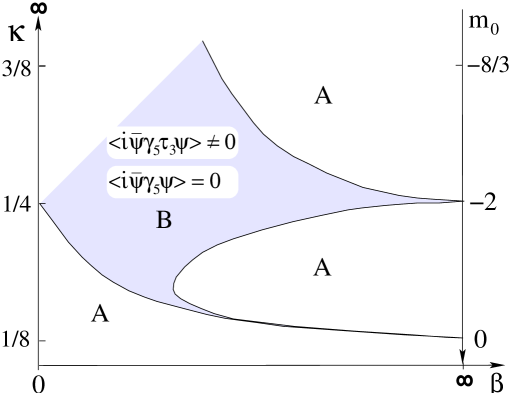
Figure 1: Aoki (B) and physical (A) region in the $(\beta,\kappa)$ plane. Adapted from [17] by courtesy of the authors.

2.1 Standard Wisdom

The standard order parameters to distinguish the Aoki region from the QCD region are $i\bar{\psi}\gamma_{5}\tau_{j}\psi$ and $i\bar{\psi}\gamma_{5}\psi$, with $\tau_{j}$ the three Pauli matrices. For the standard election, $j=3$, they can be written as a function of the up and down quark fields as follows

$$i\bar{\psi}\gamma_{5}\tau_{3}\psi =i\bar{\psi}_{u}\gamma_{5}\psi_{u}-i\bar{\psi}_{d}\gamma_{5}\psi_{d},$$ (2)

$$i\bar{\psi}\gamma_{5}\psi =i\bar{\psi}_{u}\gamma_{5}\psi_{u}+i\bar{\psi}_{d}\gamma_{5}\psi_{d}.$$

The standard wisdom for the Aoki phase can be summarized by the following two equations [4]

$$\langle i\bar{\psi}\gamma_{5}\tau_{3}\psi\rangle \neq 0,$$ (3)

$$\langle i\bar{\psi}\gamma_{5}\psi\rangle =0.$$

These equations should hold in the vacuum selected when we add a twisted mass term to the Euclidean Wilson action (1),

$$S_{m_{t}}=m_{t}i\bar{\psi}\gamma_{5}\tau_{3}\psi,$$ (4)

which breaks both parity and flavor symmetries, and take the vanishing twisted mass limit once the infinite degrees of freedom limit has been performed. The first of the two condensates $i\bar{\psi}\gamma_{5}\tau_{3}\psi$ breaks both parity and flavor symmetries. The non-vanishing vacuum expectation value of this condensate signals the spontaneous breaking of the $SU(2)$ flavor symmetry down to $U(1)$, with two Goldstone charged pions. Notwithstanding parity is spontaneously broken if the first equation in (3) holds, the vacuum expectation value of the flavor diagonal condensate $\langle i\bar{\psi}\gamma_{5}\psi\rangle$ vanishes. Indeed it is also an order parameter for a discrete symmetry $P^{\prime}$, composition of parity and discrete flavor rotations, which is assumed to be realized [11].

The Aoki phase can then be characterized by the presence of two massless charged pions and a massive neutral pion which becomes massless just at the critical line separating this phase from the physical one. In addition the $\eta$-meson, the mass of which can be extracted from the long distance behavior of the two-point correlation function of the flavor singlet pseudoscalar operator $i\bar{\psi}\gamma_{5}\psi$, stays massive even at the critical line as a consequence of the $U(1)_{A}$ axial anomaly.

2.2 Our alternative Scenario

Three years ago this standard scenario was revised in [21] with the help of the probability distribution function (PDF) of the parity-flavor fermion bilinear order parameters [28][29]. We found that if the spectral density $\rho_{U}(\lambda,\kappa)$ of the overlap Hamiltonian $\gamma_{5}W(\kappa)$, or Hermitian Dirac-Wilson operator, in a fixed background gauge field $U$ were not symmetric in $\lambda$ in the thermodynamic limit for the relevant gauge configurations, Hermiticity of $i\bar{\psi}_{u}\gamma_{5}\psi_{u}+i\bar{\psi}_{d}\gamma_{5}\psi_{d}$ would be violated at finite $\beta$. Assuming that the Aoki phase ends at finite $\beta$, this would imply the loss of any physical interpretation of this phase in terms of particle excitations. If on the contrary the spectral density $\rho_{U}(\lambda,\kappa)$ of the Hermitian Dirac-Wilson operator in a fixed background gauge field $U$ is symmetric in $\lambda$, we argued in [21] on the appearance of other phases, which can be characterized by a non-vanishing vacuum expectation value of $i\bar{\psi}_{u}\gamma_{5}\psi_{u}+i\bar{\psi}_{d}\gamma_{5}\psi_{d}$, and which can not be connected with the Aoki vacua by parity-flavor symmetry transformations. We summarize here the main steps of [21].

The key point was to study the Fourier transform of the PDF of the fermion bilinear order parameters, $P(q)$, defined as

$$P(q)={\frac{\int[dU][d\bar{\psi}d\psi]\exp\{-S_{YM}+\bar{\psi}W(\kappa)\psi+{\frac{iq}{V}}\int d^{4}x\>\>O(x)\}}{\int[dU][d\bar{\psi}d\psi]\exp\{-S_{YM}+\bar{\psi}W(\kappa)\psi\}},}$$ (5)

where $O$ is any fermion bilinear operator

$$O(x)=\bar{\psi}(x)\tilde{O}\psi(x),$$ (6)

with $\tilde{O}$ a matrix with Dirac, color and flavor indices, and $V$ is the number of lattice points. Integrating out the fermion fields one gets

$$P(q)={\frac{\int[dU]e^{-S_{YM}}\det(W(\kappa)+{\frac{iq}{V}}\tilde{O})}{\int[dU]e^{-S_{YM}}\det W(\kappa)},}$$ (7)

which can also be expressed as the following mean value

$$P(q)=\left\langle{\frac{\det(W(\kappa)+{\frac{iq}{V}}\tilde{O})}{\det W(\kappa)}}\right\rangle,$$ (8)

computed in the effective gauge theory with the integration measure

$$[dU]e^{-S_{YM}}\det W(\kappa).$$

The q-derivatives of $P(q)$ give us the moments of the PDF of our fermion bilinear

$${\frac{d^{n}{P(q)}}{dq^{n}}}\bigg{\rvert}_{q=0}=i^{n}\left\langle\left(\frac{1}{V}\int d^{4}x\>\>O(x)\right)^{n}\right\rangle.$$ (9)

For the case we are interested in, and if we call $P_{j}(q),P_{0}(q)$ the PDF of

$$c_{j} =i\bar{\psi}\gamma_{5}\tau_{j}\psi,$$ (10)

$$c_{0} =i\bar{\psi}\gamma_{5}\psi.$$

In momentum space, we have

$$P_{1}(q)=P_{2}(q)=P_{3}(q) =\left\langle\prod_{j}\left(-{\frac{q^{2}}{V^{2}\lambda_{j}^{2}}}+1\right)\right\rangle,$$ (11)

$$P_{0}(q) =\left\langle\prod_{j}\left({\frac{q}{V\lambda_{j}}}+1\right)^{2}\right\rangle,$$

where $\lambda_{j}$ are the real eigenvalues of the one flavor Hermitian Dirac-Wilson operator $\bar{W}(\kappa)=\gamma_{5}W(\kappa)$.

Since $c_{0},c_{j}$ are order parameters for the symmetries of the lattice action and we are not selecting a particular vacuum state, their first moment will vanish always, independently of the realization of the symmetries. The first non-vanishing moment, if the symmetry is spontaneously broken, will be the second:

$$\left\langle c_{0}^{2}\right\rangle =2\left\langle{\frac{1}{V^{2}}}\sum_{j}{\frac{1}{\lambda_{j}^{2}}}\right\rangle-4\left\langle\left({\frac{1}{V}}\sum_{j}{\frac{1}{\lambda_{j}}}\right)^{2}\right\rangle,$$ (12)

$$\left\langle c_{3}^{2}\right\rangle =2\left\langle{\frac{1}{V^{2}}}\sum_{j}{\frac{1}{\lambda_{j}^{2}}}\right\rangle.$$

In the QCD region flavor symmetry is realized. The PDF of $c_{3}$ will be then $\delta(c_{3})$ and $\langle c_{3}^{2}\rangle=0$. We get then

$$\left\langle c_{0}^{2}\right\rangle=-4\left\langle\left({\frac{1}{V}}\sum_{j}{\frac{1}{\lambda_{j}}}\right)^{2}\right\rangle,$$

which should vanish since parity is also realized in this region. Furthermore a negative value of $\langle c_{0}^{2}\rangle$ would violate Hermiticity of $i\bar{\psi}\gamma_{5}\psi$.

In the Aoki region [4] there are vacuum states in which the condensate $c_{3}$ (10) takes a non-vanishing vacuum expectation value. This implies that the PDF $P(c_{3})$ will not be $\delta(c_{3})$ and therefore $\langle c_{3}^{2}\rangle$ (12) will not vanish. Indeed expression (12) for $\langle c_{3}^{2}\rangle$ seems to be consistent with the Banks and Casher formula [30] which relates the spectral density of the Hermitian Dirac-Wilson operator at the origin with the vacuum expectation value of $c_{3}$ [11].

If, on the other hand, $\langle i\bar{\psi}\gamma_{5}\psi\rangle=0$ in one of the Aoki vacua, as conjectured in [4], $\langle i\bar{\psi}\gamma_{5}\psi\rangle=0$ in all the other vacua that are connected with the standard Aoki vacuum by a parity-flavor transformation, since $i\bar{\psi}\gamma_{5}\psi$ is invariant under flavor transformations and changes sign under parity. Therefore if we assume that these are all the degenerate vacua, we should conclude that $P(c_{0})=\delta(c_{0})$ and $\langle c_{0}^{n}\rangle=0$, which would imply an infinite tower of non-trivial relations, one for each even moment of the PDF. We write here the simplest one,

$$\left\langle{\frac{1}{V^{2}}}\sum_{j}{\frac{1}{\lambda_{j}^{2}}}\right\rangle=2\left\langle\left(\frac{1}{V}\sum_{j}{\frac{1}{\lambda_{j}}}\right)^{2}\right\rangle\neq 0.$$ (13)

A possible scenario which was discussed in [21] is the one that emerges if we assume a symmetric distribution for the eigenvalues of the Hermitian Wilson operator. As discussed in [21] this assumption is necessary in order to preserve Hermiticity. If we take this assumption in the most naive way we get

$$\langle c_{3}^{2}\rangle-\langle c_{0}^{2}\rangle=4\left\langle\left(\frac{1}{V}\sum_{j}{\frac{1}{\lambda_{j}}}\right)^{2}\right\rangle=0,$$ (14)

and therefore we should conclude that new vacua characterized by a non-vanishing vacuum expectation value of the singlet flavor pseudoscalar operator $i\bar{\psi}\gamma_{5}\psi$ must exist besides the Aoki vacua. Nevertheless as Sharpe noticed in [22], sub-leading contributions to the spectral density may affect equation (14) in the $\epsilon$-regime in such a way that, not only $\langle c_{0}^{2}\rangle$, but every even moment of $i\bar{\psi}\gamma_{5}\psi$ would vanish, restoring the standard Aoki picture.

As we will show in this article equation (14) turns out not to be realistic in the Aoki phase, as follows from numerical simulations. However the thesis of Sharpe, although possible and inspired in the absence of our conjectured new vacua in the chiral effective Lagrangian approach, would enforce as discussed before an infinite series of sum rules, similar to those found by Leutwyler and Smilga in the continuum [31]. The main purpose of this paper is to clarify these issues.

2.3 Some interesting relations

As previously discussed flavor and parity symmetries should be realized in the vacuum of the physical phase. This phase can therefore be characterized, in what concerns its low energy spectrum, by the existence of three degenerate massive pions, which become massless at the critical line, and the $\eta$-meson, which is massive even at the critical line because of the axial anomaly. When we cross the critical line and enter into the Aoki phase, the neutral pion becomes massive whereas the charged pions are massless since they are the two Goldstone bosons associated to the spontaneous breaking of the $SU(2)$ flavor group to a $U(1)$ group.

The susceptibilities of the neutral pion $\chi_{\pi^{0}}$ and the $\eta$-meson $\chi_{\eta}$ in the physical phase are the corresponding integrated two-point correlation functions

$$\chi_{\pi^{0}}= \sum_{x}\left\langle i\bar{\psi}\gamma_{5}\tau_{3}\psi\left(x\right)i\bar{\psi}\gamma_{5}\tau_{3}\psi\left(0\right)\right\rangle = \frac{2}{V}\left\langle\sum_{i=1}^{V}\frac{1}{\lambda_{i}^{2}}\right\rangle,$$ (15)

$$\chi_{\eta}= \sum_{x}\left\langle i\bar{\psi}\gamma_{5}\psi\left(x\right)i\bar{\psi}\gamma_{5}\psi\left(0\right)\right\rangle\textrm{} = \frac{2}{V}\left\langle\sum_{i=1}^{V}\frac{1}{\lambda_{i}^{2}}\right\rangle-\frac{4}{V}\left\langle\left[\sum_{i=1}^{V}\frac{1}{\lambda_{i}}\right]^{2}\right\rangle.$$ (16)

The rightmost hand sides of these equations are just the second moments of the PDF of $i\bar{\psi}\gamma_{5}\tau_{3}\psi$ and $i\bar{\psi}\gamma_{5}\psi$ (see equations (12)) multiplied by the corresponding volume factor. Therefore equations (15) and (16) give us the following relation between $\chi_{\eta}$, $\chi_{\pi^{0}}$ and the trace of the inverse one flavor Hermitian Dirac–Wilson operator:

$$\chi_{\eta}=\chi_{\pi^{0}}-{4\over V}\left\langle Tr^{2}\left(\gamma_{5}W^{-1}\left(\kappa\right)\right)\right\rangle,$$ (17)

to be compared with the well known relation between the eta, pion and topological susceptibilities

$$\chi_{\eta}=\chi_{\pi^{0}}+4{\chi_{T}\over m^{2}},$$ (18)

which holds in the continuum and also in the Ginsparg-Wilson regularization at finite lattice spacing.

The first interesting observation that follows from equations (17) and (18) is the suggestive relation between the topological susceptibility $\chi_{T}$ and the trace of the inverse Hermitian Dirac–Wilson operator,

$${\chi_{T}\over m^{2}}=-{1\over V}\left\langle Tr^{2}\left(\gamma_{5}W^{-1}\left(\kappa\right)\right)\right\rangle,$$ (19)

which should hold near the continuum limit. This suggests also the following relation between the trace of the inverse Hermitian Dirac–Wilson operator, quark mass $m$, and the density of topological charge $q=Q/V$ [32, 33]

$${q\over m}={1\over V}Tr\left(\gamma_{5}W^{-1}\left(\kappa\right)\right),$$ (20)

A second interesting observation that follows from (17) concerns the behavior of

$${4\over V}\left\langle Tr^{2}\left(\gamma_{5}W^{-1}\left(\kappa\right)\right)\right\rangle=\frac{4}{V}\left\langle\left[\sum_{i=1}^{V}\frac{1}{\lambda_{i}}\right]^{2}\right\rangle$$ (21)

when we approach the critical line from the physical phase. Indeed in the physical phase this quantity should be finite because the pion and eta susceptibilities are finite. However when approaching the critical line it should diverge in order to compensate the divergence of the pion susceptibility keeping $\chi_{\eta}$ finite in (17), in deep similarity with the divergence of the topological susceptibility divided by the square quark mass in the continuum and Ginsparg–Wilson regularization in the chiral limit. The origin of this divergence lies in the accumulation of eigenvalues of the Hermitian Dirac–Wilson operator near the origin.

The divergence of (21) at the critical line is slower than $V$ in such a way as to keep a parity-flavor symmetric vacuum, as corresponds to a second order phase transition. On the other hand if the standard scenario for the Aoki phase is realized, the higher accumulation of eigenvalues of the hermitian Dirac-Wilson operator at the origin in this phase should be enough to give a finite contribution to $\left\langle c^{2}_{i}\right\rangle$ (second equation in (12)). Indeed if the Aoki vacuum selected with a twisted mass term plus those obtained by parity-flavor symmetry transformations are the only degenerate vacua in this phase, the following relation should hold [22, 28]

$$\left\langle c_{3}^{2}\right\rangle={\Sigma^{2}\over 3},$$ (22)

where $\Sigma$ is the mean value of $c_{3}$ in the vacuum selected by the twisted mass term. In Section 5 we will report the results of a check of equation (22).

The standard scenario for the Aoki phase requires also that the singlet flavor pseudoscalar operator $i\bar{\psi}\gamma_{5}\psi$ takes a vanishing vacuum expectation value. Taking into account the first equation in (12), this requirement implies that the l.h.s. of eq. (21), ${4\over V}\left\langle Tr^{2}\left(\gamma_{5}W^{-1}\left(\kappa\right)\right)\right\rangle$, should diverge as $V$, to compensate the first contribution to $\left\langle c^{2}_{0}\right\rangle$ in (12).

2.4 Spontaneous Symmetry Breaking of P’?

Years ago Sharpe and Singleton suggested [11] that a symmetry $P^{\prime}$, composition of parity and flavor transformations, associated to a discrete subgroup of the parity-flavor continuous group, and acting on pure gluonic operators as parity, could still be realized in the Aoki phase, notwithstanding parity and flavor are spontaneously broken in this phase. Their motivation for such a proposal was the attempt to reconcile the Vafa–Witten theorem [34] on the impossibility to break spontaneously parity in a vector-like theory, with the existence of the Aoki phase. Their point was that Vafa–Witten theorem, although it does not apply to fermionic order parameters, could still apply to pure gluonic operators. Then if the realization of $P^{\prime}$ does not require a vanishing Aoki condensate, and $P^{\prime}$ acts on pure gluonic operators as parity, the existence of the Aoki phase besides the realization of $P^{\prime}$ in the vacuum would not be in conflict with the Vafa–Witten theorem for pure gluonic operators. Furthermore the realization of $P^{\prime}$ would be quite useful since it would give a simple explanation for the tower of sum rules (13) required in the standard scenario. Indeed the flavor singlet pseudoscalar condensate $i\bar{\psi}\gamma_{5}\psi$ is an order parameter for $P^{\prime}$.

Although the main motivation for the introduction of the $P^{\prime}$ symmetry, the realization of Vafa–Witten theorem for pure gluonic operators, has become less relevant on the light of later works on this subject [35]-[38], the implications on the standard scenario for the Aoki phase of the realization of this symmetry are still relevant.

A possible election for $P^{\prime}$, the realization of which would not be in conflict with non-vanishing condensates $\left\langle i\bar{\psi}\gamma_{5}\tau_{j}\psi\right\rangle$ for $j=1,2,3$ is the composition of parity with the $Z_{4}$ subgroup of the $SU(2)$ flavor group generated by

$${i\over{\sqrt{3}}}\left(\tau_{1}+\tau_{2}+\tau_{3}\right).$$

In this context let us consider the operator

$$Q={1\over V}Tr\left(\gamma_{5}W^{-1}\left(\kappa\right)\right)=\frac{1}{V}\sum_{j=1}^{V}\frac{1}{\lambda_{j}},$$ (23)

which is a non-local order parameter for $P^{\prime}$. This operator, although non-local, is not singular since exact zero modes have vanishing integration measure in the Wilson formulation. We will assume in what follows that $Q$ is an intensive operator. Notice that any local operator should be intensive but any intensive operator is not necessarily local. Our assumption is based in the following argument: $\left\langle Q\right\rangle={1\over 2V}\left\langle\sum_{x}\bar{\psi}(x)\gamma_{5}\psi(x)\right\rangle$, $\bar{\psi}(x)\gamma_{5}\psi(x)$ being a local fermionic operator. Our prejudices tell us that ${1\over 2V}\sum_{x}\bar{\psi}(x)\gamma_{5}\psi(x)$, as any intensive operator, should be self-averaging. In other words, if the system size is very large, a single thermalized gauge configuration should be enough to get ${1\over 2V}\left\langle\sum_{x}\bar{\psi}(x)\gamma_{5}\psi(x)\right\rangle$, and this seems indeed to be the case in the physical phase, where the PDF of $Q$ approaches a delta, as shown in Section 4. Furthermore equations (17) and (18) strongly suggest that, near the continuum limit, $Q$ would be essentially the density of topological charge, which indeed is an intensive operator.

Hence were the $P^{\prime}$ symmetry realized in the vacuum, the PDF of (23) would be, according to our assumption, a $\delta(x)$ distribution. But the second moment of this PDF,

$$\frac{1}{V^{2}}\left\langle\left[\sum_{i=1}^{V}\frac{1}{\lambda_{i}}\right]^{2}\right\rangle,$$

needs to be finite in the standard scenario for the Aoki phase in order to realize the first sum rule (13). Therefore the standard scenario requires the spontaneous symmetry breaking of $P^{\prime}$, but then there are no symmetry reasons to justify this tower of sum rules. In Section 4 we will report numerical results for the PDF of (23), both in the Aoki and in the physical phase.

3 The simulations

In order to determine the phase structure and the properties of the vacuum, we need to measure the $PDFs$ of the parity-flavor order parameters described in the previous sections, including the $Q$ operator (23). So we decided to carry out HMC simulations of QCD with two flavors of Wilson fermions, inside and outside the Aoki phase, and mainly without external sources, although some simulations with a twisted mass term in the action have also been performed.

We remove the external sources because of several facts:

1. The PDF formalism requires the removal of any external sources in the action. We just perform one long simulation in the Gibbs state.

2. The addition of a twisted mass external source, as has been done in past simulations of the Aoki phase, automatically selects the vacuum where the standard properties of the Aoki phase are verified [21]. This point could explain why no one ever saw a new Aoki phase like the one we are proposing, since all the past simulations performed with two flavors of Wilson fermions inside the Aoki phase were done with an external twisted mass term.

3. We could try to select one of these hypothetical new vacua by adding an external source proportional to $i\bar{\psi}\gamma_{5}\psi$, but this introduces a severe sign problem in the simulations.

The Aoki phase without external sources is very hard to simulate. Inside the Aoki phase there are exactly massless pions and quasi-zero modes, rendering the condition number of the Wilson Dirac operator quite high. A standard solver will not be enough to invert the Dirac operator in a HMC simulation. Fortunately, in recent years a number of efficient solvers have appeared, and by using a DD–HMC [39] we could invert the Dirac operator at a reasonable speed with the resources available to us, i.e., the clusters of the department of theoretical physics of the University of Zaragoza, comprising 160 cores and 280 Gb of available memory, interconnected by a gigabit network. The simulations were parallelized for 4, 8 or 12 cores using openMP, and we did several simultaneous runs. The iteration count of the solver ranged from a handful outside the Aoki phase, to a few hundred inside the Aoki phase in the largest volume $8^{4}$ and without external sources. For volumes higher than $8^{4}$, the inversion time became prohibitive for our computing resources and our time-frame, and we should look for new ways of simulating the Aoki phase.

Moreover, there is an additional problem with these simulations: since quasi-zero modes appear inside the Aoki phase, the eigenvalues sometimes attempt to cross the origin, and they would do so, were it not for the fact that the crossing of eigenvalues is forbidden by the HMC dynamics: the potential energy in the molecular dynamics step diverges at the origin, and there is an infinite repulsion that prevents the eigenvalues from crossing.

In order to solve this problem we classified our simulations according to its sector number, i.e., the number of ’crossed’ eigenvalues of the Hermitian Dirac–Wilson operator they had: beginning from a completely symmetric state (same number of positive and negative eigenvalues), the number of the eigenvalues that should cross to reach the desired state; and we performed simulations with a different number of crossed eigenvalues for each volume. Now this does not completely solve the problem, since we still don’t know the weight of each sector within the partition function. The only way to simulate dynamically all the sectors is to add a twisted mass term, but as explained above we are primarily interested in the results without external sources. Fortunately the weights of the different sectors evolve very slowly with the twisted mass, and we can then extrapolate the data to vanishing twisted mass.

Indeed in Table 1 we report the weights of the different sectors as a function of the volume and twisted mass $m_{t}$. Qch stands for quenched, whereas the numbers marked as MFA come from an $MFA$ (Microcanonical Fermion Average) inspired approach [40], and were obtained by diagonalizing $4\times 10^{6}$ gauge configurations. As can be seen in this table the weights show a very mild $m_{t}$-dependence, although the $4^{4}$ results at $m_{t}=0$ obtained from $MFA$ simulations are at two standard deviations from the extrapolated results. It is not clear to us if this discrepancy has a statistical origin or reflects a discontinuity of the weights of different sectors at $m_{t}=0$. However if the latter were the actual case, the standard picture for the Aoki phase could not be realized since it requires continuity in the sample of relevant gauge configurations at $m_{t}=0$. Hence we will assume continuity of the weights, and in the following sections we will use Table 1 to reconstruct the PDF for the interesting bilinears by summing the weighted PDFs of all sectors for a given volume. The details of the runs can be checked in Table 2.

Vol.	$m_{t}$	Sector 0	Sector 1	Sector 2	Sector 3+
$4^{4}$	MFA	$80\%\pm 6\%$	$20\%\pm 6\%$	$0\%$	$0\%$
$4^{4}$	$0.01$	$68.1\%\pm 1.0\%$	$31.6\%\pm 1.0\%$	$0.24\%\pm 0.08\%$	$0\%$
$4^{4}$	$0.05$	$70.4\%\pm 0.3\%$	$29.4\%\pm 0.3\%$	$0.18\%\pm 0.07\%$	$0\%$
$4^{4}$	$0.10$	$69.3\%\pm 0.9\%$	$30.4\%\pm 0.9\%$	$0.28\%\pm 0.04\%$	$0\%$
$4^{4}$	$0.30$	$70.3\%\pm 0.7\%$	$29.6\%\pm 0.6\%$	$0.14\%\pm 0.05\%$	$0\%$
$4^{4}$	$0.50$	$70.0\%\pm 0.5\%$	$29.8\%\pm 0.5\%$	$0.20\%\pm 0.06\%$	$0\%$
$4^{4}$	Qch	$71.4\%\pm 0.3\%$	$28.5\%\pm 0.2\%$	$0.07\%\pm 0.02\%$	$0\%$
$6^{4}$	$0.01$	$51.8\%\pm 0.6\%$	$44.7\%\pm 0.7\%$	$3.3\%\pm 0.3\%$	$0\%$
$6^{4}$	$0.05$	$49.9\%\pm 0.8\%$	$45.7\%\pm 0.4\%$	$4.3\%\pm 0.5\%$	$0.08\%\pm 0.02\%$
$6^{4}$	$0.10$	$51.4\%\pm 0.6\%$	$44.7\%\pm 0.6\%$	$3.86\%\pm 0.07\%$	$0.06\%\pm 0.02\%$
$6^{4}$	$0.30$	$52.7\%\pm 1.2\%$	$44.3\%\pm 1.0\%$	$2.96\%\pm 0.20\%$	$0.06\%\pm 0.06\%$
$6^{4}$	$0.50$	$53.1\%\pm 0.6\%$	$44.0\%\pm 0.5\%$	$2.82\%\pm 0.18\%$	$0.06\%\pm 0.02\%$
$6^{4}$	Qch	$55.0\%\pm 1.6\%$	$43.0\%\pm 1.9\%$	$2.0\%\pm 0.4\%$	$0\%$
$8^{4}$	$0.05$	$36.0\%\pm 0.6\%$	$48.2\%\pm 0.7\%$	$13.9\%\pm 0.4\%$	$2.06\%\pm 0.20\%$
$8^{4}$	$0.10$	$36.1\%\pm 0.6\%$	$47.0\%\pm 0.4\%$	$14.6\%\pm 0.3\%$	$2.22\%\pm 0.28\%$
$8^{4}$	$0.30$	$38.2\%\pm 0.4\%$	$46.8\%\pm 0.4\%$	$13.33\%\pm 0.12\%$	$1.6\%\pm 0.4\%$
$8^{4}$	$0.50$	$39.0\%\pm 0.3\%$	$48.5\%\pm 0.3\%$	$11.33\%\pm 0.25\%$	$1.18\%\pm 0.11\%$

Table 1: Weights of the different sectors as a function of the volume and $m_{t}$.

Vol.	$\beta$	$\kappa$	$m_{t}$	Sector	Confs	Acc ($\%$)	HMC Step	$l_{Traj}$
$4^{4}$	$2.00$	$0.25$	$0.00$	$0$	$5000$	$99\%$ $(72\%)$	3.125e-03	0.1
$4^{4}$	$2.00$	$0.25$	$0.00$	$1$	$2473$	$99\%$ $(73\%)$	2.5e-03	0.1
$6^{4}$	$2.00$	$0.25$	$0.00$	$0$	$676$	$92\%$ $(60\%)$	6.25e-04	0.04
$6^{4}$	$2.00$	$0.25$	$0.00$	$1$	$2000$	$88\%$ $(56\%)$	6.25e-04	0.04
$4^{4}$	$4.00$	$0.18$	$0.00$	$All^{\star}$	$10000$	$92\%$	0.1	1.0
$6^{4}$	$4.00$	$0.18$	$0.00$	$All^{\star}$	$5000$	$84\%$	0.1	1.0
$8^{4}$	$4.00$	$0.18$	$0.00$	$All^{\star}$	$5000$	$74\%$	0.1	1.0
$4^{4}$	$2.00$	$0.25$	$0.01$	$All$	$5001$	$83\%$	0.0133	0.2
$4^{4}$	$2.00$	$0.25$	$0.05$	$All$	$5001$	$86\%$	0.05	0.4
$4^{4}$	$2.00$	$0.25$	$0.10$	$All$	$5664$	$92\%$	0.025	0.5
$4^{4}$	$2.00$	$0.25$	$0.30$	$All$	$4999$	$96\%$	0.1	0.5
$4^{4}$	$2.00$	$0.25$	$0.50$	$All$	$10000$	$99\%$	0.025	0.5
$6^{4}$	$2.00$	$0.25$	$0.01$	$All$	$2520$	$99\%$ $(89\%)$	0.01	0.4
$6^{4}$	$2.00$	$0.25$	$0.05$	$All$	$5000$	$70\%$	0.05	0.4
$6^{4}$	$2.00$	$0.25$	$0.10$	$All$	$5000$	$95\%$	0.05	0.4
$6^{4}$	$2.00$	$0.25$	$0.30$	$All$	$5001$	$90\%$	0.1	0.5
$6^{4}$	$2.00$	$0.25$	$0.50$	$All$	$5001$	$99\%$	0.05	0.4
$8^{4}$	$2.00$	$0.25$	$0.05$	$All$	$5001$	$77\%$	0.04	0.2
$8^{4}$	$2.00$	$0.25$	$0.10$	$All$	$5001$	$84\%$	0.05	0.5
$8^{4}$	$2.00$	$0.25$	$0.30$	$All$	$5001$	$96\%$	0.05	0.4
$8^{4}$	$2.00$	$0.25$	$0.50$	$All$	$10000$	$98\%$	0.05	0.5

Table 2: Details of the simulations that generated our configurations. The word Sector refers to the eigenvalue sector where the simulation was performed, as explained above. The ^⋆ means that only sector 0 contributes in this case, so all sectors were taken into account. Also, Confs refers to the number of configurations saved (we saved one configuration for each two generated, so as to reduce the autocorrelations), Acc is the acceptance ratio of the simulation (the value in parenthesis marks the acceptance without the replay trick), HMC Step is the molecular dynamics time-step used (during replays, the step was halved) and $l_{Traj}$ is the trajectory length used.

The high variability of the acceptance ratio is due to the hard task of fine-tuning the solver parameters and the trajectory length to work properly for each case. As the table shows, certain simulations required a very small time-step for the HMC to work; in those simulations the eigenvalues were trying to cross the origin, generating high forces in the molecular dynamics, and thence creating a high rejection rate, so this small time-step was strictly necessary to obtain reasonable data. To enhance acceptance, we introduced the replay trick in the hardest calculations, i.e., those inside the Aoki phase and without a twisted mass term. During replays, the stepsize was halved whereas the trajectory length was kept constant.

In order to calculate the PDF’s we diagonalized the Hermitian Dirac–Wilson operator on all configurations generated and found the eigenvalues. The diagonalizations were carried out by using a parallelized Lanczos algorithm, combined with a Sturm bisection. The algorithm was checked heavily against the LAPACK library before starting production to ensure that our results were correct, but our algorithm was much faster than the LAPACK standard diagonalization procedure for Hermitian matrices, and used a small fraction of the memory, because in our algorithm the fermionic matrix was generated on-the-fly. The diagonalization times ranged from around a few seconds for the $4^{4}$ to a few hours in the case of the $8^{4}$ on our 12 core machines.

4 Probability Distribution Function of $Q$

First of all, we checked the behavior of the PDF of the operator $Q$ outside the Aoki phase (point at $\beta=4.0$ and $\kappa=0.18$) in the three volumes considered ($4^{4}$, $6^{4}$ and $8^{4}$). As figure 2 clearly indicates, the operator $Q$ behaves as an intensive operator, as expected, and its PDF tends to a Dirac delta at the origin as the volume increases, showing that both parity and $P^{\prime}$ symmetries are realized in the vacuum of the physical phase.

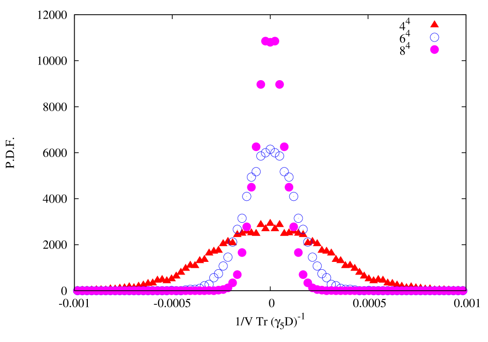
Figure 2: PDF of operator $Q$ outside the Aoki phase for three different volumes.

Let’s see what happens inside the Aoki phase ($\beta=2.0$ and $\kappa=0.25$, and for this case we will use data from the $4^{4}$ and $6^{4}$ volumes (the $8^{4}$ inside the Aoki phase was very expensive for us). We see in figure 3 and figure 4 how the PDF behaves quite differently depending on the volume and on the sector. However, when we compute the final result taking into account the weight of each sector, we see in figure 5 how all these different plots converge to a single peak of constant width, in remarkable contrast with the results in the physical phase reported in figure 2. Therefore we expect, according to our discussion in Section 2.4, that not only parity but also $P^{\prime}$ will be spontaneously broken inside the Aoki phase. We should notice that this result needs to hold if the standard picture of the Aoki phase is correct, since otherwise $\langle c^{2}_{0}\rangle=\langle c^{2}_{3}\rangle\neq 0$ in this phase.

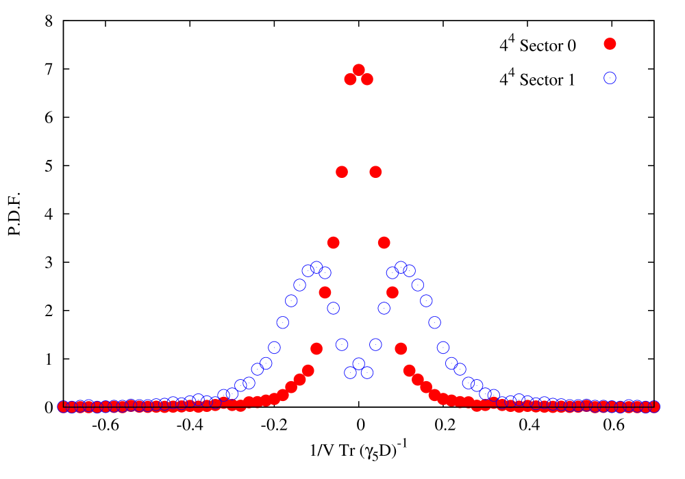
Figure 3: PDF of operator $Q$ inside the Aoki phase for the two sectors considered in the $4^{4}$ case. The sector 1 clearly shows a double peaked behavior

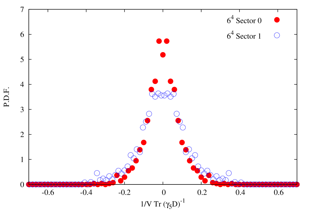
Figure 4: PDF of operator $Q$ inside the Aoki phase for the two sectors considered, now in the $6^{4}$ volume. The double peak of sector 1 becomes narrower, but we should expect wider contributions from higher sectors.

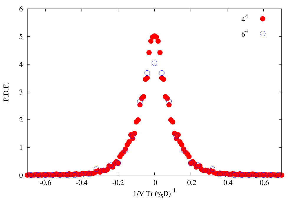
Figure 5: PDF of operator $Q$ inside the Aoki phase for two different volumes. The differences in the area can be explained by realizing that sector 2 is missing in the $6^{4}$ volume, which should account for a 5% of the area.

Of course we are far from the thermodynamic limit, and one might argue that, as stated in Table 1, the contribution of sector 2 to the $6^{4}$ volume is important enough to be taken into account. This sector was not simulated because it was extremely expensive from the numerical point of view, and since its weight is less than $5\%$, we don’t expect any changes to be relevant to the final result.

Another indication that there are new vacua inside the Aoki phase not considered in the standard picture, comes from measuring the PDF of the operator $Q$ on configurations dynamically generated with several values of an external twisted mass term, $m_{t}i\bar{\psi}\gamma_{5}\tau_{3}\psi$, but keeping $m_{t}=0$ in the definition of $Q$. Since the addition of an external source selects a standard Aoki vacuum, we expect that all the contributions to the PDF coming from the other vacua will be removed. As we can see in figure 6, the PDF for this case is essentially different than the one shown in figure 5.

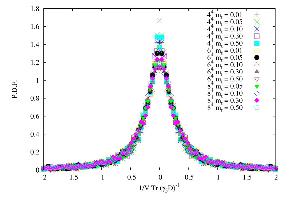
Figure 6: PDF of operator $Q$ inside the Aoki phase for configurations generated with a twisted mass source.

First of all, the PDF seems to be independent of the value of the external field. We might appreciate a slight dependence on the volume, since it seems that the peak height decreases as $V$ increases, but this effect is too small to be significant, and in any case it is a good approximation to say that the distribution is also independent of the volume. Comparing this distribution with the former one (Gibbs state, without external source, figure 5), we notice that the PDF of the operator with external source is much wider, and we then expect the spectrum to be different as well. The essential difference lies in the low modes of the Dirac operator: in the case without external source, there is a lower bound given by $1/V$ for the modulus of any eigenvalue, whereas at $m_{t}\neq 0$ the eigenvalues can become arbitrarily small . Since the PDF depends strongly on the spectrum of the Dirac operator, we expect the cases $m_{t}=0$ and $m_{t}\neq 0$ to be inherently different.

We think that this result is the strongest indication of additional vacua structure in the Aoki phase outside the standard picture. Indeed the results of figure 7 clearly show that the sample of gauge configurations obtained in the Aoki phase at $m_{t}=0$ is qualitatively different from the sample obtained at $m_{t}\neq 0$, even in the $m_{t}\rightarrow 0$ limit. On the other hand the differences in the samples can never come from the additional standard Aoki vacua since if we change the twisted mass term in the dynamical generation by any other symmetry breaking term selecting other standard Aoki vacuum, for instance $im_{t}\bar{\psi}\gamma_{5}\tau_{1,2}\psi$, the fermion determinant does not change.

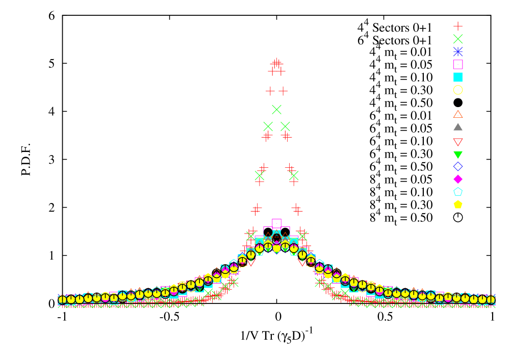
Figure 7: PDF of operator $Q$ inside the Aoki phase for all configurations. Comparison of the case $m_{t}\neq 0$ versus the case $m_{t}=0$.

5 Second moments of the PDFs of fermion bilinears

Since $P^{\prime}$ is broken according to our results plus the assumption that $Q$ is an intensive operator, the symmetry arguments supporting the existence of a tower of sum rules are no longer valid, thus it is natural to explore if the expectation value $\left\langle\left(i\bar{\psi}\gamma_{5}\psi\right)^{2}\right\rangle$ will be non-zero in the Gibbs state inside the Aoki phase. This observable is extremely difficult to measure, nonetheless we managed to obtain sensible results from our data, which we show in Table 3. As already stated in Section 3, these results assume continuity of the weights of the different sectors when $m_{t}\rightarrow 0$.

Volume	$\left\langle\left(i\bar{\psi}_{u}\gamma_{5}\psi_{u}\right)^{2}\right\rangle$	$\left\langle\left(i\bar{\psi}\gamma_{5}\psi\right)^{2}\right\rangle$	$\left\langle\left(i\bar{\psi}\gamma_{5}\tau_{3}\psi\right)^{2}\right\rangle$	$\langle Q^{2}\rangle$
$4^{4}$ Sector 0	$\left(1.93\pm 0.02\right)\times 10^{-2}$	$\left(2.51\pm 0.07\right)\times 10^{-2}$	$\left(5.23\pm 0.09\right)\times 10^{-2}$	$\left(6.8\pm 0.3\right)\times 10^{-3}$
$6^{4}$ Sector 0	$\left(2.15\pm 0.05\right)\times 10^{-2}$	$\left(2.82\pm 0.18\right)\times 10^{-2}$	$\left(5.76\pm 0.13\right)\times 10^{-2}$	$\left(7.4\pm 0.6\right)\times 10^{-3}$
$4^{4}$ Sector 1	$\left(6.0\pm 0.5\right)\times 10^{-3}$	$\left(-5.5\pm 0.5\right)\times 10^{-2}$	$\left(7.9\pm 0.4\right)\times 10^{-2}$	$\left(3.34\pm 0.20\right)\times 10^{-2}$
$6^{4}$ Sector 1	$\left(1.75\pm 0.09\right)\times 10^{-2}$	$\left(0.4\pm 0.4\right)\times 10^{-2}$	$\left(6.56\pm 0.26\right)\times 10^{-2}$	$\left(1.53\pm 0.15\right)\times 10^{-2}$
$4^{4}$ Total	$\left(1.50\pm 0.03\right)\times 10^{-2}$	$\left(-0.6\pm 1.9\right)\times 10^{-3}$	$\left(6.08\pm 0.19\right)\times 10^{-2}$	$\left(1.54\pm 0.08\right)\times 10^{-3}$
$6^{4}$ Total	$\left(1.81\pm 0.12\right)\times 10^{-2}$	$\left(1.27\pm 0.29\right)\times 10^{-2}$	$\left(6.0\pm 0.3\right)\times 10^{-2}$	$\left(1.17\pm 0.13\right)\times 10^{-3}$

Table 3: Interesting v.e.v. for the Aoki phase in the different sectors. Only statistical errors are shown.

The fourth column in this table refers to $\left\langle\left(i\bar{\psi}\gamma_{5}\tau_{3}\psi\right)^{2}\right\rangle$, the landmark of the Aoki phase. As we see, it is clearly non-zero for all the volumes, confirming that our simulations lie within the Aoki phase. The second column shows the values for $\left\langle\left(i\bar{\psi}_{u}\gamma_{5}\psi_{u}\right)^{2}\right\rangle$, which is an order parameter for parity, but it takes into account just one flavor (which we labeled $u$). This quantity should be non-zero inside the parity-breaking Aoki phase, regardless of the discussion of the new vacua. Finally, the most important observable, the flavor singlet pseudoscalar $\left\langle\left(i\bar{\psi}\gamma_{5}\psi\right)^{2}\right\rangle$, which –since we are dealing with two degenerate flavors, $u$ and $d$– is the sum of two of the former condensates $i\bar{\psi}_{u}\gamma_{5}\psi_{u}+i\bar{\psi}_{d}\gamma_{5}\psi_{d}$. The standard picture of the Aoki phase predicts zero expectation value of this parameter in any Aoki vacuum, whereas each one of the pseudoscalars restricted to one flavor $i\bar{\psi}_{u,d}\gamma_{5}\psi_{u,d}$ will be non-zero due to parity breaking. Hence, the standard picture of the Aoki phase enforces an antiferromagnetic ordering of the pseudoscalars $i\bar{\psi}_{u}\gamma_{5}\psi_{u}=-i\bar{\psi}_{d}\gamma_{5}\psi_{d}$, which is not required in our hypothesis of the new vacua. The data of the third column in Table 3 show a clear non-zero expectation value in the case of the largest volume $6^{4}$, supporting our previous discussion regarding $P^{\prime}$ breaking.

$V$	$m_{t}$	$\left\langle i\bar{\psi}\gamma_{5}\tau_{3}\psi\right\rangle$
$4^{4}$	$0.01$	$\left(56.00\pm 0.06\right)\times 10^{-2}$
$4^{4}$	$0.05$	$\left(65.149\pm 0.022\right)\times 10^{-2}$
$6^{4}$	$0.01$	$\left(53.603\pm 0.015\right)\times 10^{-2}$
$6^{4}$	$0.05$	$\left(66.888\pm 0.008\right)\times 10^{-2}$
$8^{4}$	$0.05$	$\left(66.953\pm 0.007\right)\times 10^{-2}$
$4^{4}$	$0.10$	$\left(75.512\pm 0.009\right)\times 10^{-2}$
$6^{4}$	$0.10$	$\left(76.291\pm 0.004\right)\times 10^{-2}$
$8^{4}$	$0.10$	$\left(76.307\pm 0.003\right)\times 10^{-2}$
$4^{4}$	$0.30$	$\left(92.214\pm 0.005\right)\times 10^{-2}$
$6^{4}$	$0.30$	$\left(92.309\pm 0.002\right)\times 10^{-2}$
$8^{4}$	$0.30$	$\left(92.311\pm 0.002\right)\times 10^{-2}$
$4^{4}$	$0.50$	$\left(96.225\pm 0.003\right)\times 10^{-2}$
$6^{4}$	$0.50$	$\left(96.241\pm 0.001\right)\times 10^{-2}$
$8^{4}$	$0.50$	$\left(96.243\pm 0.001\right)\times 10^{-2}$

Table 4: Evolution of the v.e.v. of the Aoki parameter as a function of the twisted mass external field.

Concerning equation (22), which relates the mean value of the square Aoki condensate in the Gibbs state ($\epsilon$-regime) with the expectation value of this order parameter in the vacuum selected by a twisted-mass term ($p$-regime), and since we have data for the Aoki condensate at several lattice sizes and twisted masses (see Table 4), we can check its plausibility. This is a relevant test since, as discussed in Section 2.3, equation (22) should be realized in the standard Aoki scenario [28, 22]. To this end we report in figure 8 our results for the Aoki condensate at several values of the twisted-mass, $m_{t}$, in $4^{4},6^{4}$ and $8^{4}$ lattices. The circles in the ordinates axis stand for the values of the Aoki condensate at $m_{t}=0$ in $4^{4}$ and $6^{4}$ lattices, obtained from equation (22), and using as input our results for $\left\langle(i\bar{\psi}\gamma_{5}\tau_{3}\bar{\psi})^{2}\right\rangle$ reported in Table 3. The figure, which is a Fisher plot [41], shows that any reliable extrapolation of the data to $m_{t}=0$ gives a value for the Aoki condensate larger than the one obtained from equation (22).

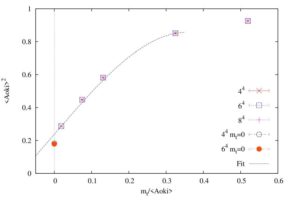
Figure 8: Fisher plot of the evolution of the v.e.v. of the Aoki parameter as a function of the twisted mass external field. The circles show the prediction obtained from the simulations in the Gibbs state (see eq.(22)). The fit shown is meant to guide the eye, and shouldn’t be taken as a prediction of the behavior of the v.e.v. of the Aoki parameter. The fit should be more reliable for small values of $m_{t}$.

One could argue that, at the volumes we are working, the finite size effects should be large and noticeable, and that the inclusion of these effects could lead to an agreement between our measurements at $m_{t}=0$ and $m_{t}\neq 0$. Nonetheless, the data at $m_{t}=0$ –which we expect to suffer more these finite volume effects due to the existence of massless pions– reveals that these effects are not very large, for the value of the Aoki condensate remains very stable after a fivefold increase in the volume.

6 Relation with $W\chi PT$

The results reported in this paper on the vacuum structure of the Aoki phase do not agree, as follows from the previous sections, with the predictions of $W\chi PT$ of Sharpe and Singleton [11] for this phase. Since $W\chi PT$ has been successfully applied in many contexts, it is worthwhile to analyze the possible origins of this discrepancy.

First one should notice that the chiral effective Lagrangian is based on the continuum effective Lagrangian written as a series of contributions proportional to powers of the lattice spacing $a$, plus the construction of the corresponding chiral effective Lagrangian, keeping only the terms up to order $a^{2}$ [11]. This means that predictions based on the use of this chiral effective Lagrangian should work close enough to the continuum limit, where keeping terms up to order $a^{2}$ can be justified. However our investigation of the Aoki phase has been done at $\beta=2.0$, and a very rough estimation gives a lattice spacing at this $\beta$ of order $3.0\;\text{GeV}^{-1}$. Hence a possible explanation for the discrepancies found relies on the necessity of including higher order terms in the chiral effective Lagrangian.

The second point to notice is that our simulations were performed deep in the Aoki phase ($\kappa=0.25$) and hence far away from the critical line where the neutral pion is massless. The chiral effective Lagrangian approach is based on the assumption that the relevant low energy degrees of freedom are the three pions. This assumption is very reliable in the physical phase near the critical line, and also in the Aoki phase near the critical line, but it could break down as we go deep in the Aoki phase, as is our case. To better understand this point we have analyzed the two flavor Nambu-Jona Lasinio model with Wilson fermions in the mean field approximation not only with the standard action [42, 43] but with the more general action with an $SU(2)_{V}\times SU(2)_{A}\times U(1)_{B}$ symmetry. The continuum Euclidean Lagrangian density for this model is

$${\cal L}=-\bar{\psi}\left(\not{\partial}+m\right)\psi+G_{1}\left[\left(\bar{\psi}\psi\right)^{2}+\left(i\bar{\psi}\gamma_{5}{\vec{\tau}}\psi\right)^{2}\right]+G_{2}\left[\left(i\bar{\psi}\gamma_{5}\psi\right)^{2}+\left(\bar{\psi}{\vec{\tau}}\psi\right)^{2}\right]$$ (24)

This model regularized on a hypercubic four-dimensional lattice with Wilson fermions was analyzed at $G_{2}=0$ in the mean field or first order $1/N$ expansion by Bitar and Vranas [42] and Aoki et al. [43], who found a phase, for large values of $G_{1}$, in which both, flavor symmetry and parity, are spontaneously broken, in close analogy to lattice QCD with Wilson fermions.

The Nambu-Jona Lasinio model given by action (24) enjoys the same $SU(2)_{V}\times SU(2)_{A}\times U(1)_{B}$ symmetry of $QCD$ and it is an effective model to describe the low energy physics of $QCD$ [44]. As stated before we have analyzed the phase diagram of this model in the mean field approach in the three parameters space ($\kappa$, $G_{1}$, $G_{2}$), and a detailed report of our results will appear in a forthcoming publication. What we want to point out here is that whereas in the large $G_{1}$ and small $G_{2}$ region the results on the phase diagram agree with those obtained in [43] and therefore with the standard Aoki picture, at larger values of $G_{2}$ we find phases where the flavor singlet pseudoscalar condensate $i\bar{\psi}\gamma_{5}\psi$ takes a non-vanishing vacuum expectation value, including phases with vacua degenerated with the standard Aoki vacua, and which can not be connected with the Aoki vacua by parity-flavor symmetry transformations. This example shows that the complete phase diagram of a model having the same chiral, vector and discrete symmetries as $QCD$, cannot be understood assuming that chiral symmetry is realized in the standard strong interaction Goldstone picture.

7 The condensates near the $m_{0}=-4.0$ line of the phase diagram

The phase diagram of lattice QCD with two degenerate flavors of Wilson fermions in the bare fermion mas, $m_{0}$, and gauge coupling, $g^{2}$, plane is symmetric under the $m_{0}\rightarrow-(m_{0}+8)$ change. At the invariant point, $m_{0}=-4$, the system shows extra symmetries. Indeed, if we parameterize the bare fermion mass as $m_{0}=-4+\epsilon$, the fermionic Wilson action for one flavor can be written as

$${S_{F}}=\epsilon\sum_{x}\bar{\psi}(x)\psi(x)-{1\over 2}\sum_{x,\mu}\left(\bar{\psi}(x)(1+\gamma_{\mu})U^{+}_{\mu}(x-\mu)\psi(x-\mu)+\right.\\ \left.\bar{\psi}(x)(1-\gamma_{\mu})U_{\mu}(x+\mu)\psi(x+\mu)\right)$$ (25)

and at $\epsilon=0$ ($m_{0}=-4$) we have an extra global $Z(4)$ symmetry for each flavor, generated by the following transformations

$$\psi^{\prime}(x)=(-1)^{x_{1}+x_{2}+x_{3}+x_{4}}i\psi(x)$$

$$\bar{\psi}^{\prime}(x)=\bar{\psi}(x)(-1)^{x_{1}+x_{2}+x_{3}+x_{4}}i$$ (26)

These symmetries enforce, in the two flavor model, the equality of the condensates

$$\langle\left(i\bar{\psi}\gamma_{5}\tau_{3}\psi\right)^{2}\rangle=\langle\left(i\bar{\psi}\gamma_{5}\psi\right)^{2}\rangle$$ (27)

and since the standard wisdom on the phase diagram of this model, corroborated on the other hand by the strong coupling and large number of colors expansion of [3, 4], tells us that $\epsilon=0$ is in the Aoki phase for any value of the gauge coupling, we should conclude that there exists at least a line in the phase diagram, $\epsilon=0$, along which both condensates take a non-vanishing identical value. Notice also that these non-vanishing condensates imply the spontaneous breaking of not only parity and flavor symmetries, but also the $Z(4)$ symmetries (26).

On a finite lattice, the two condensates (27) can be described by the ratio of two even polynomials of $\epsilon$, and a simple Taylor expansion would suggest that the two condensates do not vanish in a region of non-vanishing measure of the phase diagram, thus giving a qualitative picture consistent with the numerical results reported in this article. However the actual situation can be more complex, since we can not exclude a priori that the convergence radius of the $\epsilon$-expansion vanishes in the infinite volume limit. This convergence radius is given by the distance to the origin of the nearest zero of the partition function in the complex $\epsilon$-plane, and the scaling of these zeroes with the lattice volume is related to the chiral condensate $\bar{\psi}\psi$, in a similar way as the zeroes of the partition function of the staggered formulation in the complex mass plane are related to the realization of the chiral symmetry for staggered fermions. This analogy comes from the fact that at $\epsilon=0$ the chiral condensate in the Wilson formulation vanishes due to the $Z(4)$ symmetry, in the same way as the chiral condensate in the staggered formulation vanishes at zero fermion mass because of chiral symmetry. Also, the behavior of the chiral condensate when $\epsilon\rightarrow 0$, is controlled by the scaling of the zeroes of the partition function in the complex $\epsilon$ plane with the lattice volume. A singular condensate at $\epsilon=0$ will be obtained if the zeroes of the partition function approach the point $\epsilon=0$ with the lattice volume. On the contrary, if the scaling of the zeroes stops at finite distance, an analytical value for the chiral condensate will be obtained.

The solution of this problem outside approximations is a very hard task. However the dependence of the chiral condensate on $\epsilon$ was computed by Aoki in the strong coupling and large N expansion in [3, 4], the final result being

$${{\langle\bar{\psi}\psi\rangle}\over{8N}}={{3\epsilon}\over{16-\epsilon^{2}}}$$ (28)

for $0\leq\epsilon^{2}<4$. Equation (28) shows that the chiral condensate is an analytical function of $\epsilon$ in the strong coupling limit, and that the convergence radio of the $\epsilon$-power expansion is 2. Hence we should expect the same analyticity domain for the other two condensates (27).

These results show that, at least in the strong coupling and large N approximation, we should expect a phase structure for QCD with two flavors of Wilson fermions as the one proposed by us, giving theoretical support to the numerical results reported in this article.

8 Conclusions and Outlook

Three years ago the standard scenario for the phase structure of lattice QCD with two degenerate flavors of Wilson fermions was revised by three of us in [21], where we conjectured on the appearance of new vacua in the Aoki phase, which can be characterized by a non-vanishing vacuum expectation value of $i\bar{\psi}_{u}\gamma_{5}\psi_{u}+i\bar{\psi}_{d}\gamma_{5}\psi_{d}$, and which can not be connected with the Aoki vacua by parity-flavor symmetry transformations. However, Sharpe pointed out in [22] that the standard picture for the Aoki phase can be understood using the chiral effective theory appropriate to the Symanzik effective action, and that within this standard analysis, the flavor singlet pseudoscalar expectation value vanishes, $\left\langle i\bar{\psi}\gamma_{5}\psi\right\rangle=0$. As the standard scenario for the Aoki phase is indeed a direct consequence of the $W\chi PT$ application to this phase, we were also calling into question in [21] the validity of the $W\chi PT$ analysis, at least for low values of $\beta$, and therefore large values of the lattice spacing $a$. These issues are relevant enough to make it worthwhile to continue these investigations in order to clarify the actual scenario for the Aoki phase.

For the last few years we have performed an extensive research on the vacuum structure of the Aoki phase, in order to find out if our alternative vacuum structure, derived from a PDF analysis, was realized or not. These simulations, which have been mainly performed in the absence of any parity-flavor symmetry breaking external source, are plagued by technical difficulties which have been responsible for the slow progress in the field. Indeed the addition of a twisted mass external source, as it has been done in the past simulations of the Aoki phase, automatically selects the vacuum where the standard properties of the Aoki phase are verified. This point could explain why nobody ever saw a new phase like the one we are proposing, since all the past simulations performed with two flavors of Wilson fermions inside the Aoki phase were done within an external twisted mass term.

Notwithstanding these difficulties, we have provided in this work evidence pointing to a more complex vacuum structure in the Aoki phase of two flavor QCD, as conjectured in [21]. Indeed the results reported in Table 3, which were obtained under the assumption that the weights of the different sectors are continuous at $m_{t}=0$, show how we were able to perform a direct measurement of $\left\langle\left(i\bar{\psi}\gamma_{5}\psi\right)^{2}\right\rangle$ in the Aoki phase, which gave a non-zero value for this operator in the $6^{4}$ lattice, of the same order of magnitude as $\left\langle\left(i\bar{\psi}_{u}\gamma_{5}\psi_{u}\right)^{2}\right\rangle$, and $\left\langle\left(i\bar{\psi}\gamma_{5}\tau_{3}\psi\right)^{2}\right\rangle$, the last two being non-vanishing in the Aoki phase in the standard scenario. Thus this result points to the breaking of the hypothesis of the sum-rules (13). Furthermore a check of equation (22), a equation which should hold if the standard scenario for the Aoki phase is realized, reported in figure 8, points out to a more complex vacuum structure too.

However the strongest indication, in our opinion, on the existence of a vacuum structure in the Aoki phase, more complex than the one of the standard picture, comes from our analysis of the PDF of the operator $Q$ (23). Our motivation for the analysis of this kind of density of ”topological charge” operator, which measures the asymmetries in the eigenvalue distribution of the Hermitian Dirac–Wilson operator, was twofold. First it appears in the computation of the second moment of the PDF of the flavor singlet pseudoscalar order parameter (12), and second $Q$ is an order parameter for the symmetry $P^{\prime}$, composition of parity and discrete flavor transformations, described in Section 2.

Our numerical results for the PDF of $Q$, together with the assumption that $Q$ is an intensive operator, suggest that the $P^{\prime}$ symmetry is realized in the vacuum of the physical phase, but not in the Aoki phase, at least in the strong coupling region we have analyzed. However the cleanest signal of further structure in the Aoki phase comes from the results on the PDF of $Q$ reported in figure 7. Those results clearly show that the sample of gauge configurations obtained in the Aoki phase at $m_{t}=0$ is qualitatively different from the sample obtained at $m_{t}\neq 0$, since they give incompatible PDF’s. Furthermore this result stays true in the $m_{t}\rightarrow 0$ limit, as follows from the independence of the shape of the PDF of $Q$ on the twisted mass $m_{t}$. On the other hand the differences in the samples can never come from the additional standard Aoki vacua since if we change the twisted mass term in the dynamical generation by any other symmetry breaking term selecting other standard Aoki vacuum, as for instance $im_{t}\bar{\psi}\gamma_{5}\tau_{1,2}\psi$, the fermion determinant does not change.

As the sum rules (13) required in the standard scenario are only supported, as discussed before, by the $W\chi PT$ analysis of the Aoki phase, our results could call into question also the validity of the $W\chi PT$ analysis performed in [11] for low values of $\beta$ (around 2.0, very coarse lattices) and deep into the Aoki phase ($\kappa=0.25$). However, $W\chi PT$ is expected to work at higher values of $\beta$, near the continuum limit and close to the critical line. Indeed, one could be concerned that, at such a low $\beta$ and high $\kappa$, we are far from the continuum limit and from the region of applicability of the standard chiral effective Lagrangian, as discussed in Section 6. Actually the analysis done in Section 7 gives theoretical support to our alternative scenario. Nonetheless our work is devoted to the Aoki phase on the lattice, which might not even have a continuum limit.

In any case any improvement of our results in larger lattices and for more $\beta,\kappa$ values would be of great interest. Unfortunately, given the technical difficulties of the simulations inside the Aoki phase, this calculation is outside our present computing resources.

References

- [1] V. Azcoiti, A. Nakamura, Phys. Rev. D27, 2559 (1983).
- [2] H.W. Hamber, Nucl. Phys. B251, 182 (1985).
- [3] S. Aoki, Phys. Rev. D30, 2653 (1984).
- [4] S. Aoki, Phys. Rev. Lett. 57, 3136 (1986).
- [5] S. Aoki, S. Boettcher, and A. Gocksch, BNL-ABG-1; hep-lat/9312084 (1993).
- [6] M. Creutz, arXiv:hep-lat/9608024.
- [7] K.M. Bitar, Phys. Rev. D56, 2736 (1997).
- [8] S. Aoki, T. Kaneda, and A. Ukawa, Phys. Rev. D56, 1808 (1997).
- [9] K.M. Bitar, U.M. Heller, and R. Narayanan, Phys. Lett. B418, 167 (1998).
- [10] R.G. Edwards, U.M. Heller, R. Narayanan, and R.L. Singleton, Jr, Nucl. Phys. B518, 319 (1998).
- [11] S.R. Sharpe, R.L. Singleton, Jr, Phys. Rev. D58, 074501 (1998).
- [12] S. Aoki, Nucl. Phys. B (Proc. Suppl.) 60A, 206 (1998).
- [13] K. Bitar, Nucl. Phys. B (Proc. Suppl.) 63A-C, 829 (1998).
- [14] S. Sharpe, R.L. Singleton Jr, Nucl. Phys. B (Proc. Suppl) 73, 234 (1999).
- [15] R. Kenna, C. Pinto, and J.C. Sexton, Phys. Lett. B505, 125 (2001).
- [16] M. Golterman, Y. Shamir, Phys. Rev. D68, 074501 (2003).
- [17] E.M. Ilgenfritz, W. Kerler, M. Müller-Preussker, A. Sternbeck, and H. Stuben, Phys. Rev. D69, 074511 (2004).
- [18] A. Sternbeck, E.M. Ilgenfritz, W. Kerler, M. Müller-Preussker, and H. Stuben, Nucl. Phys. B (Proc. Suppl.) 129&130, 898 (2004).
- [19] M. Golterman, S.R. Sharpe, and R.L. Singleton, Jr, Nucl. Phys. B (Proc. Suppl.) 140, 335 (2005).
- [20] VE.M. Ilgenfritz, M. Müller-Preussker, M. Petschlies, K. Jansen, M.P. Lombardo, O. Philipsen, L.Zeidlewicz, and A. Sternbeck, PoS LATTICE2007, (2008) 323.
- [21] V. Azcoiti, G. Di Carlo, A. Vaquero, Phys. Rev. D79, 014509 (2009).
- [22] S. Sharpe, Phys. Rev. D79, 054503 (2009)
- [23] A. Vaquero, V. Azcoiti, G. Di Carlo, E. Follana, PoS LATTICE2009 068 (2009)
- [24] V. Azcoiti, G. Di Carlo, E. Follana, A. Vaquero, PoS LATTICE2010 091 (2010)
- [25] V. Azcoiti, G. Di Carlo, E. Follana, A. Vaquero, PoS LATTICE2011 112 (2011)
- [26] G. Akemann, P.H. Damgaard, K. Splittorff, J.J.M. Verbaarschot Phys. Rev. D83, 085014 (2011)
- [27] M. Kieburg, K. Splittorff, J.J.M. Verbaarschot, Phys. Rev. D85 (2012).
- [28] V. Azcoiti, V. Laliena, and X.Q. Luo, Phys. Lett. B354, 111 (1995).
- [29] V. Azcoiti, G. Di Carlo, and A. Vaquero, JHEP0804:035, (2008).
- [30] T. Banks, A Casher, Nucl. Phys. B169, 103 (1980).
- [31] H. Leutwyler, A. Smilga, Phys. Rev. D 46, 5607 (1992).
- [32] J. Smit, J.C. Vink, Nucl. Phys. B286, 485 (1987).
- [33] P. Hasenfratz, V. Laliena, F. Niedermayer, Phys. Lett. B427, 125 (1998).
- [34] C. Vafa, E. Witten, Phys. Rev. Lett. 53, 535 (1984).
- [35] V. Azcoiti, A. Galante, Phys. Rev. Lett. 83, 1518 (1999).
- [36] X. Ji, Phys. Lett. B554, 33 (2003).
- [37] P.R. Crompton, Phys. Rev. D 72, 076003 (2005).
- [38] V. Azcoiti, G. Di Carlo, E. Follana, A. Vaquero, JHEP1007:047, (2010).
- [39] M. Luscher, Comput. Phys. Commun. 156, (2004) 20.
- [40] V. Azcoiti, G. Di Carlo, A.F. Grillo, Phys. Rev. Lett. 65, 2239 (1990).
- [41] J.S. Kouvel, M.E. Fisher, Phys. Rev. 136, A1626 (1964).
- [42] K. M. Bitar, P. M. Vranas, Phys.Rev. D50 (1994) 3406.
- [43] S. Aoki, S. Boettcher, A. Gocksch, Phys.Lett. B331 (1994) 157.
- [44] A. Dhar, R, Shankar, and S. R. Wadia, Phys. Rev. D31, 3256 (1985).