Dynamical and stationary critical behavior of the Ising ferromagnet in a thermal gradient

Abstract

In this paper we present and discuss results of Monte Carlo numerical simulations of the two-dimensional Ising ferromagnet in contact with a heat bath that intrinsically has a thermal gradient. The extremes of the magnet are at temperatures $T_{1}<T_{c}<T_{2}$, where $T_{c}$ is the Onsager critical temperature. In this way one can observe a phase transition between an ordered phase ($T<T_{c}$) and a disordered one ($T>T_{c}$) by means of a single simulation.
By starting the simulations with fully disordered initial configurations with magnetization $m\equiv 0$ corresponding to $T=\infty$, which are then suddenly annealed to a preset thermal gradient, we study the short-time critical dynamic behavior of the system. Also, by setting a small initial magnetization $m=m_{0}$, we study the critical initial increase of the order parameter. Furthermore, by starting the simulations from fully ordered configurations, which correspond to the ground state at $T=0$ and are subsequently quenched to a preset gradient, we study the critical relaxation dynamics of the system. Additionally, we perform stationary measurements ($t\rightarrow\infty$) that are discussed in terms of the standard finite-size scaling theory.
We conclude that our numerical simulation results of the Ising magnet in a thermal gradient, which are rationalized in terms of both dynamic and standard scaling arguments, are fully consistent with well established results obtained under equilibrium conditions.
PACS Numbers : 64.60.De; 64.60.an, 05.10.-a
Keywords : Phase transitions, thermal gradient, Ising ferromagnet, numerical simulations.

1 Introduction

Let us assume that a physical system undergoes a smooth transition between two distinctly characteristic phases when a certain control parameter (e.g., $T=$ temperature, $P=$ pressure, $\mu=$ chemical potential, etc.) is finely tuned around a critical value. This physical situation is often addressed by means of analitical and numerical methods where the control parameter asuumes a fixed value. However, here we considered an alternative approach by assuming that along a given spatial direction, the system undergoes a well established gradient of the control parameter, such that the critical point lies between the extreme values, e.g., $T_{1}<T_{c}<T_{2}$, where one has a thermal gradient between temperatures $T_{1}$ and $T_{2}$, and the critical temperature $T_{c}$ is within that range dgrad0 ; dgrad1 ; dgrad2 ; dgrad3 ; jsm . Of course, a standard reversible system, usually studied under equilibrium conditions, will be out of equilibrium under the gradient constraint applied to the control parameter. However, we will show below that this situation is no longer a shortcoming for the application of methods and theories already developed for the study of equilibrium systems. In order to fix ideas, in this paper we will study the dynamical and stationary behavior of the Ising model for a two-dimensional magnetisingorig in a thermal gradient. The proposed study not only possess interesting theoretical challenges, but it may also be useful in connection to recent experimental work aimed to characterize films in general, and magnetic films in particular, which are obtained under thermal gradient conditions imposed on the substrate. In fact, since the temperature is a key parameter for the relevant properties of thin films, several experiments have focused on the influence of a temperature gradient on film growth, e.g., Tanaka et al. reported studies of magnetic Tb-Te films obtained under thermal gradient conditionstanaka . Also, Schwickert et al.aleman have introduced the temperature wedge method where a temperature gradient of several hundred Kelvin was established across a substrate during the co-deposition of Te and Pt. Other experiments performed by Xiong et al.xiong involve nanostructures obtained by using a gradient temperature.

So, within the broad context discussed above, we now focus our attention on the aim of this paper, which is to perform an extensive numerical study of the two-dimensional Ising ferromagnet in a thermal gradient. In previous numerical studies performed by various authorsdgrad0 ; dgrad1 ; dgrad2 ; dgrad3 ; jsm , the two extremes of the magnet are considered in contact with different thermal baths, e.g. the left-hand and the right-hand side extremes are at fixed temperatures $T_{1}$ and $T_{2}$, respectively. In order to study this particular out-of-equilibrium situation, varoius algorithms can be used, e.g. the Creutz algorithm dgrad0 ; creutz , the Kadanoff-Swift move KS the Q2R rule Q2R , the KQ rule dgrad2 , a recently introduced microcanonical dynamics jsm , etc. In this way, the system naturally evolves into a stationary state and a thermal gradient is established between its extremes. Also, the surfaces in the direction perpendicular to the one where the gradient is observed are surrounded by an adiabatic wall. In particular, Neek-Amal et al. dgrad1 have reported the ocurrence of an almost linear temperature gradient (c.f. figure 1 of reference dgrad1 ), for the case of the $d=2$ Ising model, by using the Creutz algorithm. On the other hand, the mean-field treatment given by the well known Fourier equation kit , namely

$$\frac{\partial^{2}T(x,t)}{\partial x^{2}}-K\;\frac{\partial T(x,t)}{\partial t}=0,$$

$$T(0,t)=T_{1},\;T(L,t)=T_{2},$$

where $T(x,t)$ is the temperature along the solid and $K$ is the (constant) thermal conductivity, predicts a linear temperature gradient between both baths. In fact, we assumed a solid of length $L$ where the gradient is applied, while the remaining directions are irrelevant. Then, in the $t\rightarrow\infty$ limit, the time-dependent contributions to the solution become negligible, and one gets the linear gradient, namely,

$$T(x)=T_{1}+\frac{(T_{2}-T_{1})}{L}\;x.$$ (1)

It is worth mentioning that the above simulation studies dgrad0 ; dgrad1 ; dgrad2 ; jsm of the Ising system are precisely focused on the calculation of the thermal conductivity, among other relevant observables, such as the energy profiles of the system’s transversal sections. Also, in all cases the discussed results were obtained under stationary conditions. However, simulation results that are in contrast to the mean-field theory, clearly show that the thermal conductivity is not a constant in these systems since it depends on the local temperature (or energy) dgrad0 ; dgrad1 ; dgrad2 ; jsm , hence the temprature may not necessarily grow linearly along the heat propagation direction. In fact, in the presence to thermal fluctuations it is expected that transport properties may exhibit non-trivial spatial patterns due to the non-equilibrium nature of the system under study jsm , and under these conditions the thermal conductivity depends on the temperature (apart from other relevant parameters of the model). In particular, for the Ising system in a thermal gradient, Agliari et al. jsm reports that $K(T)$ exhibits a peak slightly above criticality, whose position is independent of both the lattice size and the temperature difference between the extrems of the sample. Therefore, the system that we study in the present paper is not simply an Ising model where different temperatures are imposed at the bundaries, but it describes a system where the temperature gradient is present in the heat bath itself and the transport properies of the system are determined also by the bath and not only by the Ising dynamics. While the linear gradient used in our calculations is motivated by the fact that we considered a sample in contact with a thermal bath that intrinsically has a gradient, that assumption can also be supported by a physical argument. In fact, to define a thermal conductivity there must exist mechanisms such that the degrees of freedom (e.g. the phonons) dominate the thermal properties and spins locally thermalize to the temperature of the lattice. In the absence of such mechanisms the phonons at one end of the crystal will not be in thermal equilibrium at a temperature $T_{2}$, and those at the other end in equilibrium at $T_{1}$ kit . Then, if we assume that the lattice has a constant conductivity, at least in the temperature range where the magnetic transition takes place, we expect a linear growth of the temperature when a temperature difference is apllied to the extrems.

In the present paper we not only undertake a completely different approach than those used in previous studies, as already anticipated, but we are also interested in both the dynamic and the stationary behavior of a broad spectra of physical observables. In fact, we consider that the Ising ferromagnet is already in contact with a thermal bath that intrinsically has a thermal gradient along the $x-$direction, as described by equation (1). In this way each column of coordinates $x_{i}=i$, with $i=1,2,....,L$ of our two-dimensional (lattice) system, is in equilibrium with the thermal bath at temperature $T(x_{i})$. Under this condition we apply the standard Metropolis dynamics by considering the proper temperature for each column. So, the whole system reaches a stationary, non equilibrium regime, with a net flux of energy from the hotter to the colder extremes at temperatures $T_{2}$ and $T_{1}$, respectively.

As already anticipated, we are interested in the study of the dynamic behavior of the system, i.e., by addressing both the relaxation dynamics and the short-time dynamicsalbano , as well as the stationary behavior that is established in the long-time regime. By using the dynamic scaling theory albano and the finite-size scaling theory binder , both developed for the analysis of critical behavior of samples in homogeneous thermal baths, we are able to rationalize all measurements performed in our thermal gradient system. In this way we determined not only the critical temperature but also relevant critical exponents such as those of the order parameter ($\beta$), the susceptibility ($\gamma$), the correlation length ($\nu$), etc. We also show that the hyperscaling relationship given by $d^{*}-2\beta/\nu=\gamma/\nu$ holds, with an effective dimension $d^{*}=1$, which reflects the fact that the susceptibility is measured as the fluctuations of the order parameter (magnetization) per unit of length along the direction perpendicular to the gradient.

The paper is organized such that in Section 2 we provide the description of the model and the simulation method, in order to allow for a smooth introduction of the theoretical background in Section 3. In section 4 we present and discuss the results. Finally, our conclusions are stated in Section 5.

2 BRIEF DESCRIPTION OF THE ISING MAGNET IN A THERMAL GRADIENT AND THE SIMULATION METHOD

We performed simulations of the Ising model in the two-dimensional square lattice with a rectangular geometry, with a Hamiltonian given by

$$H=-J\sum_{\langle ij,i^{\prime}j^{\prime}\rangle}\,s_{i,j}s_{i^{\prime},j^{\prime}},$$ (2)

where the spin variables can assume two values, i.e. $s_{ij}=\pm 1$, $J>0$ is the coupling constant that is set positive in order to account for ferromagnetic interactions, and summation runs over nearest-neighbor sites as indicated by the symbol $\langle ij,i^{\prime}j^{\prime}\rangle$. The Ising system is an archetypal model for the study of second-order equilibrium phase transitions. In fact, it is well known that the local interactions of the Hamiltonian given by equation (2) lead to a macroscopically observable transition between an ordered ferromagnetic phase and a disordered paramagnetic one, which in $d=2$ dimensions takes place at the Onsager critical temperature $T_{c}=\frac{2J}{k_{B}\ln(1+\sqrt{2})}$onsager , where $k_{B}$ is the Boltzmann constant (hereafter we report all temperature values in units of $J/k_{B}$).

In this work we placed the Ising ferromagnet of size $L\times M$ in contact with a thermal bath that intrinsically has a thermal gradient along the $L-$direction, as given by equation (1). Therefore, each column of length $M$ located at $x=i$, with $1\leq i\leq L$, is in thermal equilibrium with the bath temperature $T(i)=T_{2}+(T_{2}-T_{1})i/L$, where $T_{1}$ and $T_{2}$ are the temperatures on the left- and right-hand sides of the magnet, respectively. Since we are interested in the study of the critical behavior, the temperatures are selected such that $T_{1}<T_{c}<T_{2}$, so that a phase transition between the ordered phase on the left-hand side and the disordered one at the right-hand side can be observed in a single simulation run. As imposed by the simulation geometry used we take periodic boundary conditions in the direction perpendicular to the gradient, while open boundary conditions are adopted for the extremes of the sample in the direction parallel to the gradient.

In order to perform the Monte Carlo simulation, a spin $s_{ij}$ selected at random and the change of the energy ($\Delta H$) involved in a flipping attempt $s_{ij}\rightarrow-s_{ij}$ are evaluated by using the Hamiltonian given by equation (2). Now, due to the applied thermal gradient, the flipping probability given by the Metropolis dynamics $W(s_{ij}\rightarrow-s_{ij})=exp(-\Delta H/k_{B}T(i))$ depends on the $i$th column ($1\leq i\leq L$) where the selected spin is located. Subsequently, the standard Monte Carlo procedure is implemented.

The upper panel of figure 1 shows a typical snapshot configuration obtained under stationary conditions by using the above-described procedure, while the lower panel shows a sketch of the linear gradient applied to the sample.

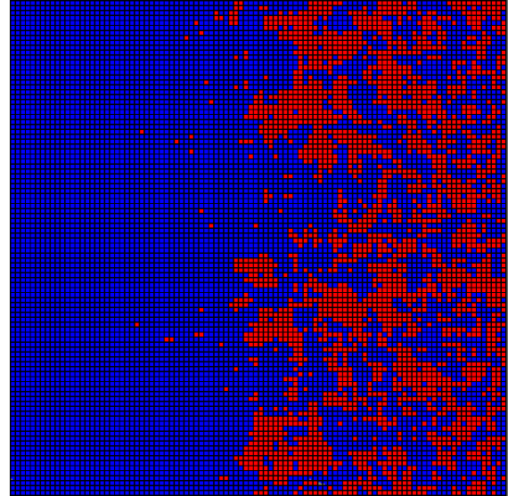
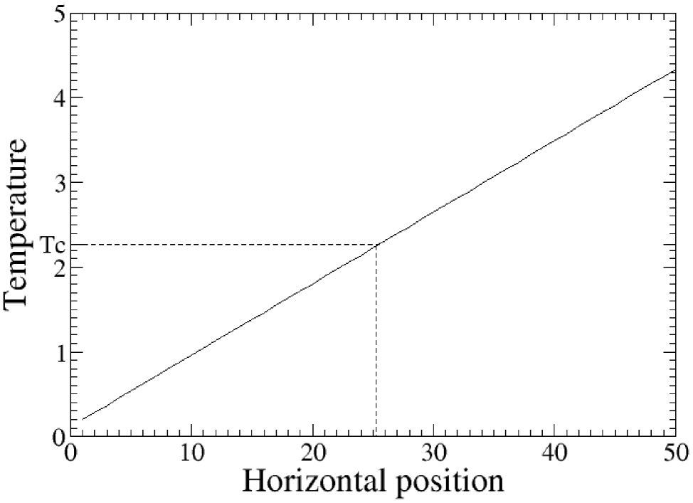
Figure 1: (Color online) The upper panel shows a typical snapshot configuration of a two-dimensional Ising ferromagnet in contact with a thermal bath that intrinsically has a linear temperature gradient that grows from $T_{1}=0.2$ (left-hand side) to $T_{2}=4.338$ (right-hand side). Up and down spins are shown in blue and red, respectively. The lower panel is a sketch of the applied gradient, showing the critical region around $T_{c}\simeq 2.269$ by means of a dotted line. The critical interphase between the ordered phase (left-hand side) and the disordered one (right-hand side) can be observed in the snapshot. More details in the text.

Due to the applied thermal gradient, all relevant physical observables depend on the coordinate running in the direction of the gradient itself, so one essentially has to measure profiles of the observables, such as the nth moment of the order parameter (magnetization in this case) is given by

$$m_{i}^{(n)}\,(T(i),x,t)=\bigg{(}\frac{1}{M}\,\sum_{j=1}^{M}\;s_{i,j}(t)\bigg{)}^{n},$$ (3)

where the dependence on the gradient axis ($1\leq i\leq L$) is explicitly indicated. Here, we have also included the time dependence, where a Monte Carlo time unit involves the random selection of $L\times M$ spins, as usual.

Furthermore, other measured observables are the susceptibility profiles, evaluated as the magnetization fluctuations, i.e.,

$$\chi_{i}(T(i),t)=\frac{1}{M}\,[m_{i}^{(2)}(T(i),t)-(m_{i}^{(1)}(T(i),t))^{2}];$$ (4)

and the second- and the fourth-order cumulants

$$U_{2}(T(i),t)=\frac{m_{i}^{(2)}(T(i),t)}{(m_{i}^{(1)}(T(i),t))^{2}}-1,$$ (5)

and

$$U_{4}(T(i),t)=1-\frac{m_{i}^{(4)}(T(i),t)}{3(m_{i}^{(2)}(T(i),t))^{2}},$$ (6)

respectively.

In order to understand the behavior of spin-spin correlations in a system in the presence of a temperature gradient, we also measured the spin-spin spatial correlation function in the direction perpendicular to the thermal gradient, defined for each column $i$ at temperature $T_{i}$ as

$$g(T_{i},r)=\frac{1}{(M-r)}\,\sum_{j=1}^{M-r}\;(\langle s_{i,j}s_{i,j+r}\rangle-\langle s_{i,j}\rangle\langle s_{i,j+r}\rangle),$$ (7)

where $r$ is the distance between spins. Furthermore, we also measured the correlation function in the direction parallel to the thermal gradient, by fixing the origin just at $T_{c}$.

For the sake of completeness it is worth mentioning that for dynamic simulations the time dependence of the already defined observables is obtained by averaging over a (large) number of different realizations ($N_{R}$) performed with different sets of random numbers and physically equivalent initial conditions. Also, measurements corresponding to the stationary regime are performed by taking averages after a large number ($N_{c}$) of different configurations, which are obtained after disregarding a (large) number ($N_{D}$) of Monte Carlo time steps, in order to allow for the system stabilization.

3 THEORETICAL BACKGROUND

By considering a fully disordered sample but with a small initial magnetization ($m_{0}$), the general scaling behavior of the n-th moment of the magnetization that it is expected to hold for temperatures close to the critical region, such that $\epsilon\equiv\frac{(T(i)-T_{c})}{T_{c}}\simeq 0$, is given byalbano ,

$$m^{(k)}(\epsilon,t,L)=b^{-\frac{k\beta}{\nu}}\tilde{m}^{(k)}(b^{-z}t,b^{\frac{1}{\nu}}\epsilon,b^{-1}L,b^{x_{0}}m_{0}),$$ (8)

where $\beta$ and $\nu$ are the order parameter and the correlation length (static) critical exponents, $z$ is the dynamic exponent, and $b$ is a suitable scaling parameteralbano . Accordingly to the short-time dynamic scaling theory, $x_{0}$ is a new exponent that governs the early-time scaling behavior of the moments of the initial magnetization. Now, by setting $b\equiv t^{1/z}$, just at the critical point ($\epsilon\equiv 0$foot0 ), and for the short-time regime such that the correlation length $\xi(t)\sim t^{1/z}$ is smaller than the typical lattice side ($\xi<L,M$) but slightly larger than the lattice spacing, one has that for $k=1$ equation (8) becomes

$$m(t)\sim t^{\theta},$$ (9)

where the exponent $\theta=\frac{x_{0}-\beta/\nu}{z}$ is the scaling exponent of the initial increase of the magnetization and equation (9) holds for $t^{x_{0}/z}\ll 1$janssen .

Furthermore, for $\epsilon=0$ and $m_{0}\equiv 0$ the scaling behavior of the fluctuations of the second moment of the magnetization, which give the susceptibility according to equation (4), is given byalbano

$$\chi(t)\sim t^{(d-2\beta/\nu)/z}.$$ (10)

It is worth mentioning that if the hyperscaling relationship $\nu d-2\beta=\gamma$ holds, one has the well-known dependence $\chi(t)\sim t^{\gamma/\nu z}$, where $\gamma$ is the susceptibility exponent.

On the other hand, by starting from a well ordered initial configuration, e.g., for $m_{0}=1$, the scaling approach given by equation (8) for $k=1$ becomes

$$m(\epsilon,t)\sim t^{-\beta/\nu z}\,\tilde{m}(t^{1/\nu z}\epsilon).$$ (11)

Therefore, just at criticality ($\epsilon\equiv 0$), one should observe a power-law decrease of the initial magnetization according tobinder

$$m(t)\sim t^{-\beta/\nu z},\;\;\;\;\epsilon=0,$$ (12)

while the logarithmic derivative of equation (11) evaluated just at criticality givesalbano

$$\frac{\partial\ln(m(t))}{\partial\epsilon}\bigg{|}_{\epsilon\equiv 0}\sim t^{1/\nu z}.$$ (13)

Finally, note that the scaling behavior of the cumulants (see equations (5) and (6)) can also be worked out by using equation (8) and one gets

$$U_{2}(t)\sim t^{d/z},\\$$ (14)

and

$$U_{4}(t)\sim t^{d/z},$$ (15)

respectively.

Summing up, by properly measuring the dynamic behavior of the system at criticality one should be able to determine the exponents, $\theta$ (equation (9)) and $(d-2\beta/\nu)z$ (equation (10)), by starting from disordered initial configurations; and $\beta/\nu z$ (equation (11)), $1/\nu z$ (equation (13)), and $d/z$ (equation (14)), by starting from ordered initial configurations.

Usually the dimensionality of the system is known so that this set of five independent determinations becomes redundant in order to evaluate four critical exponents. However, as will be shown later on, in the case of a system in a thermal gradient the complete set is essential for the determination of the effective dimensionality involved in the scaling relationships. Of course, in our gradient simulations we obtained (simultaneously and by means of single sets of simulations) information over a wide range of $T$ ($T_{1}<T_{c}<T_{2}$), while the above discussed scaling relationships are expected to hold only close to the critical region, i.e., for columns of coordinates such that $x_{c}\simeq\frac{(T_{c}-T_{1})}{(T_{2}-T_{1})}\,L$ (see equation (1)).

On the other hand, equation (8) is also useful in order to describe the stationary scaling regime. In fact, for $t\rightarrow\infty$ the value of $m_{0}$ becomes irrelevant and one gets the standard scaling relationship for the magnetization given bybinder

$$m(\epsilon,L)=L^{-\beta/\nu}\tilde{m}(\epsilon L^{1/\nu}),$$ (16)

where $\tilde{m}$ is a suitable scaling function. Furthermore, just at criticality ($\epsilon\equiv 0$) equation (16) yields

$$m(\epsilon=0)\sim L^{-\beta/\nu},$$ (17)

which reflects the fact that the magnetization vanishes at criticality in the thermodynamic limit ($L\rightarrow\infty$).

Also in the stationary limit, the spin-spin correlation function (equation (7)) has its own scaling relationship, given bykim

$$g(\epsilon=0,r)\sim r^{-(d-2+\eta)},$$ (18)

where $\eta$ is the critical exponent associated with spatial correlations, which is related to other exponents by the relationship $\gamma=\nu(2-\eta)$kim .

Furthermore, for homogeneous systems away from the critical temperature, the spin-spin correlation function exhibits an exponential decay behavior given by:

$$g(T_{i},r)\sim e^{-r/\xi_{i}},$$ (19)

where $\xi_{i}$ is the correlation length, at temperature $T_{i}$, which diverges close to criticality, according to

$$\xi_{i}\sim A\,|T_{i}-T_{c}|^{-\nu},$$ (20)

where $\nu$ is the correlation length exponent.

4 RESULTS AND DISCUSSION

Let us begin our presentation with results corresponding to dynamic measurements obtained by starting the simulations with fully ordered configurations such that $m(i,t=0)\equiv 1,\;\forall i$, which corresponds to the ground state configuration at $T=0$. By following the standard procedure the sample is suddenly quenched to the temperature of the heat bath with the proper thermal gradient. So, each column of the sample evolves, at its own temperature, towards its stationary configuration ($t\rightarrow\infty$), and in particular we focus our attention on the critical region. According to equation (8), or equivalently to equation (11), one expects to measure a power-law behavior of the physical observables just at criticality, while deviations from that type of behavior have to be found away from $T_{c}$. By plotting all the relevant measured observables ($m,\;\frac{\partial\ln(m)}{\partial(\epsilon)},\;U_{2}$ and $U_{4}$) as obtained for samples of different sizes ($100\leq L\leq 1000$), the best set of power laws is obtained for $T_{c}=2.2691(3)$foot , which is in full agreement with the Onsager critical temperatureonsager of the Ising model in $d=2$. Figure 2 shows the time dependence of the second-order cumulant (see equations (5) and (14)) as obtained close to criticality by using a square lattice of side $L=1000$. Here, the thermal gradient is set between $T_{1}=2.0$ and $T_{2}=2.4$, while the results are averaged over $N_{C}=10000$ different runs. From the best fit of the data shown in figure 2 we obtained $d/z=0.474(6)$foot .

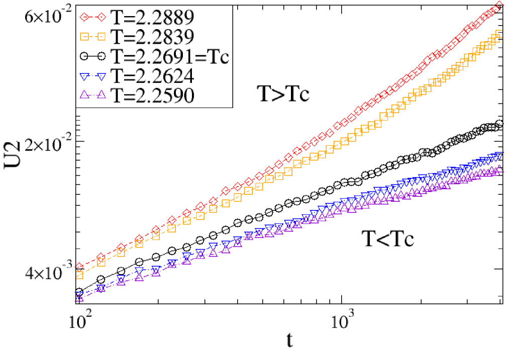
Figure 2: (Color online) Log-log plot of the second-order cumulant versus time as obtained for a lattice of side $L=1000$ and averaging over $N_{C}=10000$ different runs. The full line corresponds to the best power-law behavior that is identified as the critical point. Notice that dashed (dashed-dotted) lines show upward (downward) deviations that are typical for $T>T_{c}$ ($T<T_{c}$). The best fit of the solid line yields $d/z=0.474(6)$. More details in the text.

Our measurements obtained by using initially ordered configurations are completed by log-log plots of the time dependence of the magnetization and its logarithmic derivative, as shown in figures 3(a) and 3(b), respectively. The best plots of the lines, obtained for data corresponding to the same column that was identified with the critical temperature in figure 2, yield $\beta/\nu z=0.058(1)$foot , and $1/\nu z=0.4857(4)$foot , respectively.

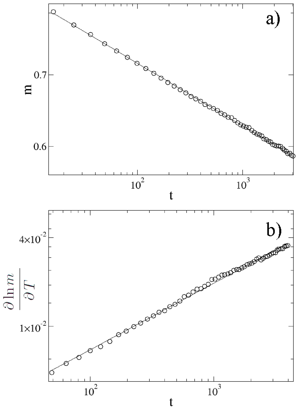
Figure 3: (a) (Upper panel) and (b) (lower panel) show log-log plots of the magnetization and its logarithmic derivative versus time, respectively. Results obtained at criticality by using samples of side $L=1000$ and by averaging over $N_{C}=10000$ different runs. In both panels the straight lines correspond to the best fits of the data shown by means of circles. The linear gradient of the thermal bath is set between $T_{1}=2.0$ and $T_{2}=2.4$. More details in the text.

On the other hand, by starting the simulations with fully disordered initial configurations such that $m_{0}=0$, which corresponds to samples in contact with a thermal bath at $T=\infty$ that are then suddenly annealed to a desired thermal gradient, we measured the time evolution of the fluctuations of the order parameter that under equilibrium conditions is identified with the magnetic susceptibility, as shown in figure 4.

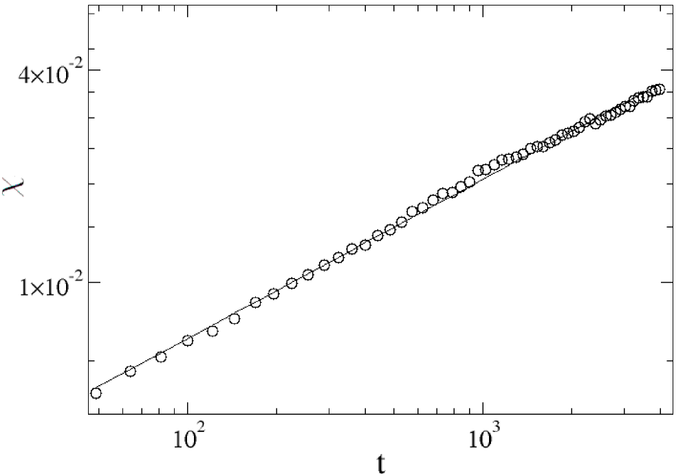
Figure 4: Log-log plot of the fluctuations of the order parameter versus $t$, as obtained for the column identified with the critical temperature in the plots shown in previous figures. Data corresponding to $L=1000$ and taking a linear gradient set between $T_{1}=2.0$ and $T_{2}=2.4$. Averages are taken over $N_{C}=10000$ different initial configurations. The best fit of the data, shown as a full line, has slope $\gamma/\nu z=0.3570(4)$.

Furthermore, initially disordered configurations with a preset (vanishing) initial magnetization are suitable for the measurement of the initial increase of the order parameter, which after the scaling arguments discussed within the context of equation (9), is expected to be observed for times such that $t<<m_{0}^{-z/x_{0}}$. Figure 5 shows log-log plots of $m$ versus $t$ as obtained for the different values of $m_{0}$ ($0.035\leq m_{0}\leq 0.050$). The data shown in figure 5 correspond to the previously identified ”critical” column. The best fits of the curves give estimates of the initial increase exponent $\theta$ that, after a proper extrapolation to the limit $m_{0}\rightarrow 0$ (not shown here for the sake of space), yields $\theta=0.196(6)$foot .

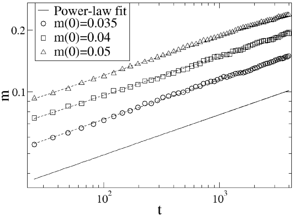
Figure 5: Log-log plot of the magnetization versus $t$, as obtained for the column identified with the critical temperature in the plots shown in previous figures. Data corresponding to $L=1000$ and taking a linear gradient set between $T_{1}=2.0$ and $T_{2}=2.4$. Averages are taken over $N_{C}=10000$ different initial configurations. Each curve corresponds to a different initial magnetization $m_{0}$, as indicated, and the dashed lines are the fits of the data. The full straight line corresponds to $\theta=0.196$, i.e. the value of the initial increase exponent obtained by extrapolation to $m_{0}\rightarrow 0$. More details in the text.

Based on the results obtained by means of dynamic measurements only, we are in a condition to outline a few interesting preliminary conclusions on the critical behavior of the Ising magnet in contact with a gradient thermal bath. On the one hand, the best fits of all physical observables were found at the same column (i.e., the same temperature) of the sample, which has been identified as the critical temperature $T_{c}=2.2691(3)$foot . This value is in full agreement with the well known exact result early evaluated by Onsager, i.e., $T_{Onsager}\simeq 2.2692$. On the other hand, by using $\beta/\nu z=0.058(1)$ and $1/\nu z=0.4857(4)$foot as determined by means of the measurements of the magnetization and its logarithmic derivative, respectively, we obtained $\beta=0.120(2)$foot , in excellent agreement with the exact value $\beta=1/8=0.125$onsager . Additionally, by assuming that the hyperscaling relationship $d\nu-2\beta=\gamma$ holds, just dividing by $\nu z$ one can write

$$\frac{d}{z}-\frac{2\beta}{\nu z}-\frac{\gamma}{\nu z}=0,$$ (21)

where equation (21) can be interpreted as a ”dynamical” hyperscaling relationship. Then, by replacing the measured exponents in equation (21) we obtain $0.001(9)$ on the right-hand of the equality, a result that strongly supports the validity of hyperscaling. On the other hand, we found that the exponent for the initial increase of the order parameter ($\theta=0.196(6)$) is in full agreement with previous numerical results obtained by applying the Metropolis dynamics to the two-dimensional Ising magnet ($d=2$) in a homogeneous bath, namely, $\theta=0.191(1)$okano . However, it should be mentioned that this exponent depends on the dynamics used (e.g. Metropolis, Glauber, Heat-Bath, etc.) and that our Gradient-Metropolis dynamics may not give the same exponents as the proper standard Metropolis dynamics.

Let us now point our attention to stationary results obtained after disregarding $N_{D}=5\times 10^{5}$ Monte Carlo steps, in order to allow for the stabilization of the sample, and evaluated during the subsequent time interval of $5\times 10^{5}$ Monte Carlo steps.

Figure 6(a) shows plots of magnetization profiles (i.e., plots of $m(i)$ versus $T_{i}$, where $T_{i}$ is the temperature of the $i$th column), as obtained for samples of different sizes. Since the temperatures at the extremes of the sample are kept constant at $T_{1}=0.64$ and $T_{2}=3.40$, each curve in figure 6(a) corresponds to different gradients. It follows that finite-size effects are negligible in the low-temperature range, e.g., for $T<2.1$, while these effects become slightly evident above criticality.

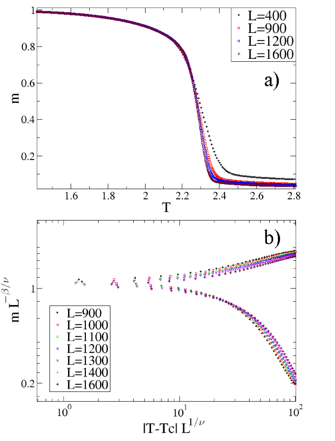
Figure 6: (Color online) (a) Plot of the magnetization profiles versus $T$ as obtained for samples of different thermal gradients. The temperatures at the extremes of the sample are $T_{1}=0.64$ and $T_{2}=3.40$, and results are averaged over $N_{D}=5\times 10^{5}$ Monte Carlo steps after disregarding the initial $5\times 10^{5}$ Monte Carlo steps in order to allow for the stabilization of the samples. (b) Scaling plots of the data already shown in (a) as obtained by using equation (16). More details in the text.

It is worth mentioning that the results shown in figure 6(a) can be replotted in order to test whether the standard scaling also holds for gradient measurements. In fact, figure 6(b) shows log-log plots of $m(T_{i},L)L^{\beta/\nu}$ versus $|T_{i}-T_{c}|L^{1/\nu}$ as obtained by using the data already shown in figure 6(a). The quality of the collapse supports the validity of the standard scaling Ansatz for the case of our gradient measurements; however, the terms of correction to scaling, which are neglected in our analysis, cannot be disregarded. On the other hand, just by selecting the critical column one has that equation (17) simply gives the monotonic decay of the magnetization when the system size is increased, namely $m(T=T_{c})\sim L^{-\beta/\nu}$, a result that has been verified in figure 7 where the best fit of the data corresponds to $\beta/\nu=0.125(9)$foot .

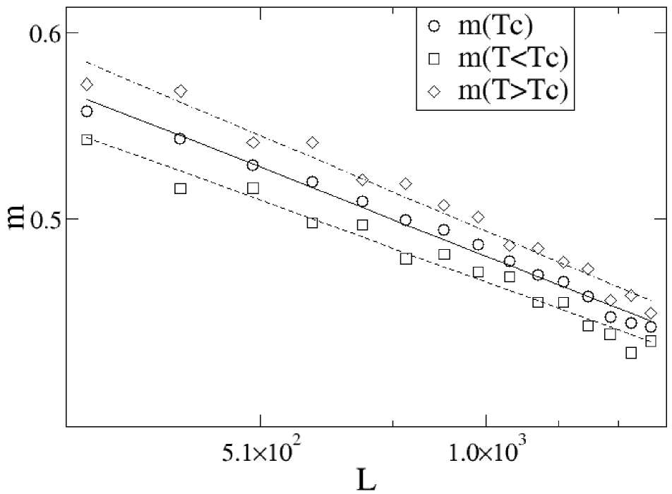
Figure 7: Log-log plot of the magnetization, measured close to criticality, versus the system side $L$. Data corresponding to the critical column (open circles), and two adjacent columns: $T<T_{c}$, open squares, and $T>T_{c}$, open diamonds, respectively. Results obtained by averaging over $5\times 10^{5}$ Monte Carlo steps after disregarding the first $N_{D}=5\times 10^{5}$ Monte Carlo steps in order to allow for the stabilization of the system. The full line has slope $-\beta/\nu=0.125(9)$, and corresponds to the best fit of the data. The other two lines correspond to the fits of the data from adjacent columns and give the error bars to the resultfoot . More details in the text.

As already established in the field of critical phenomena, the so-called cumulants (see equations (5) and (6)) are suitable functions of the moments of the order parameter distribution function whose pre-scaling factor, disregarding high-order finite-size scaling corrections, is independent of the system size. So, plots of the cumulants versus the control parameter (i.e., the temperature of the gradient thermal bath) should exhibit a common intersection point, as it is indicated with full straight vertical lines in the data shown in figures 8(a) and 8(b), obtained with our gradient system for $U_{2}(L,T)$ and $U_{4}(L,T)$, respectively. A careful inspection of the critical region close to the interaction points reveals very small but systematic shifts of the intersection points between curves corresponding to adjacent system sizes. After proper extrapolation of the intersection points to the thermodynamic limit (not shown here for the sake of space), we obtain $T_{c}(\infty)=2.284(1)$foot and $T_{c}(\infty)=2.283(3)$foot , for data corresponding to $U_{2}$ and $U_{4}$, respectively.

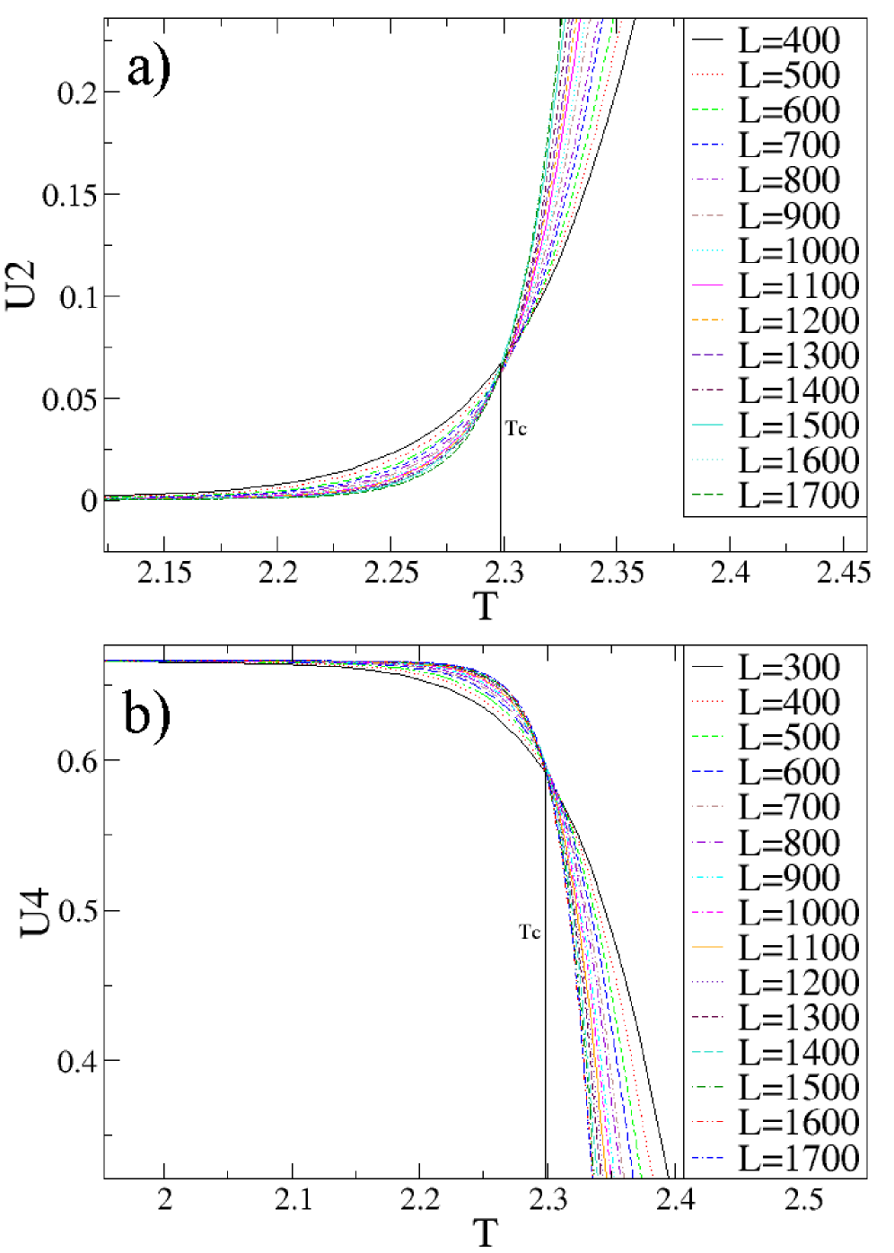
Figure 8: (Color online) Plots of the second- (a) and fourth-order (b) cumulants $U_{2}$ and $U_{4}$ versus the temperature of the column, as obtained for different values of the system side $L$ as indicated. The vertical straight lines on each graph indicate the intersection points and are shown for the sake of comparison.

On the other hand, plots of the fluctuations of the order parameter, which are identified with the susceptibility in standard measurements, show peaks close to criticality as expected (see figure 9). In fact, it is known that the susceptibility exhibits rounding and shifting effects as the size-dependent ”critical” temperature of the peaks ($T_{c}(L)$) converges toward the true critical temperature according to a standard finite-size scaling relationship given bybinder

$$T_{c}(L)=T_{c}(\infty)+constant\,L^{-1/\nu}.$$ (22)

So, the inset of figure 9 shows plots of $T_{c}(L)$ versus $L^{-1}$ (here we assume $\nu=1$ for the correlation length exponent as justified below) that yield $T_{c}(\infty)=2.296(1)$foot .

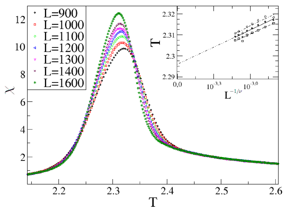
Figure 9: (Color online) Plots of the fluctuations of the magnetization versus the temperature of the column, obtained by means of simulations with systems of different side, as listed in the figure. The inset shows the extrapolation of the effective ”critical” temperature according to equation (22), which yields $T_{c}(\infty)=2.296(1)$ as the best fit (open circles). Notice that extrapolation of data corresponding to the columns adjacent to the critical one are also included, such that open diamonds and open squares correspond to $T<T_{c}$ and $T>T_{c}$, respectively. More details in the text.

In additional simulations, we studied the spin-spin correlation functions, both parallel and perpendicular to the gradient direction. We measured the correlation function in the perpendicular direction, by using equation (7) for different temperatures, both lower and higher than $T_{c}\simeq 2.26918$. We used a rectangular lattice of size $L=300$, $M=4000$, and set the temperatures of the extremes of the sample at $T_{1}=0.8$ and $T_{2}=3.74$, respectively. For each measurement corresponding to a certain temperature outside criticality, we plotted the correlation function versus the distance $r$, in log-linear plots as shown in figure 10(a). Then, by fitting the data to an exponential decay, according to equation (19), we obtained the values of the correlation length $\xi_{i}(|T_{i}-T_{c}|)$. The inset of figure 10(a) shows a linear-linear plot of $\xi(T)$ versus $1/(T-T_{c})$ that yields a straight line. This behavior confirms that equation (20) holds with $\nu=1$, and from the slope we also obtained the prefactor given by $A=1.16(4)$.

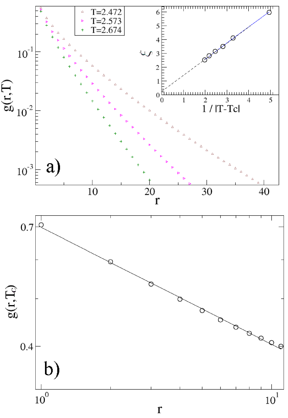
Figure 10: (Color online) (a) Log-linear plots of the vertical spin-spin correlation function $g(T,r)$ versus the distance $r$. Different curves correspond to different temperatures away from criticality, as indicated. For each curve an exponential decay fit was made, obtaining values of the correlation length $\xi(T)$. The inset in (a) shows the values of $\xi$ versus $1/|T-T_{c}|$. The linear fit indicates that equation (20) holds, with an exponent $\nu=1$. Furthermore, the slope of the fit gives us the value of the pre factor $A$ in equation (20), which is found to be $A=1.16(4)$. (b) Log-log plot of $g(T,r)$ versus $r$, as obtained for the critical temperature, with its corresponding power-law fit (full line). The exponent obtained corresponds to $d-2+\eta=0.238(3)$. A rectangular lattice was used, with $L=300$ and $M=4000$. The temperature gradient was set between $T_{1}=0.8$ and $T_{2}=3.74$. Results obtained by averaging over $5\times 10^{5}$ Monte Carlo steps after disregarding the first $N_{D}=5\times 10^{5}$ Monte Carlo steps in order to allow for the stabilization of the system. More details in the text.

On the other hand, for the correlation function corresponding to the column of the system with temperature closest to $T_{c}\simeq 2.26918$, we performed a power-law fit versus the distance $r$, according to equation (18) (see figure 10(b)), which yields $d-2+\eta=0.238(3)$. By eliminating the value of $d$ from the exponent equation with the use of relationship $d\nu-2\beta=\gamma$, and by using values already calculated from both stationary and dynamic simulations, we obtained $\eta=1.22(1)$. This value is in excellent agreement with $\eta=5/4=1.25$, found by taking $d=1$ in the relationship that results from combining $\gamma=\nu(2-\eta)$ and $d\nu-2\beta=\gamma$ with the exact exponent values of the two-dimensional Ising Model, i.e., $\nu=1$ and $\beta=1/8$onsager .

On the other hand, the correlation function in the direction parallel to the thermal gradient has also been measured, by using a system of $L=5000$ and $M=100$, with a gradient between temperatures $T_{1}=0.8$ and $T_{2}=3.74$, respectively. The correlation function studied corresponds to $g(T,r)$ at the critical temperature, namely, $g(T_{c},r)$. It is worth mentioning that correlations along the direction of the applied gradient involve spins at different temperatures, so a quantitative study such as the one done for vertical correlations is no longer possible. Instead, we gain an insight into the qualitative behavior of the Ising ferromagnet in a thermal gradient. In fact, figure 11 shows $g(T_{c},r)$ versus the distance $r$. For $r>0$, we found that correlations between the spins in the critical column and those placed in columns at higher temperatures are almost negligible. On the other hand, for $r<0$ correlations between the spins located in the critical column and those placed in columns at lower temperatures are measured. Here, the correlations first abruptly decrease and then they become almost constant for colder temperatures. The inset in figure 11 shows a log-log plot of a zoomed view of the area near criticality, where absolute values of $r$ were taken, in order to account for both branches of $g(r)$, namely, for $r>0$ and $r<0$, respectively. The full line is a plot of a power-law decay with exponent $1/4=0.25$ and is shown for the sake of comparison. By comparing the measured points with the full line, it can be inferred that close enough to the critical column correlations have a functional behavior in agreement with the well known scaling law $r^{-(d-2+\eta)}$. This result reflects the fact that for the considered gradient $\frac{\Delta T}{\Delta L}=0.588\times 10^{-3}$, the region close to $r=0$ is almost at the critical temperature.

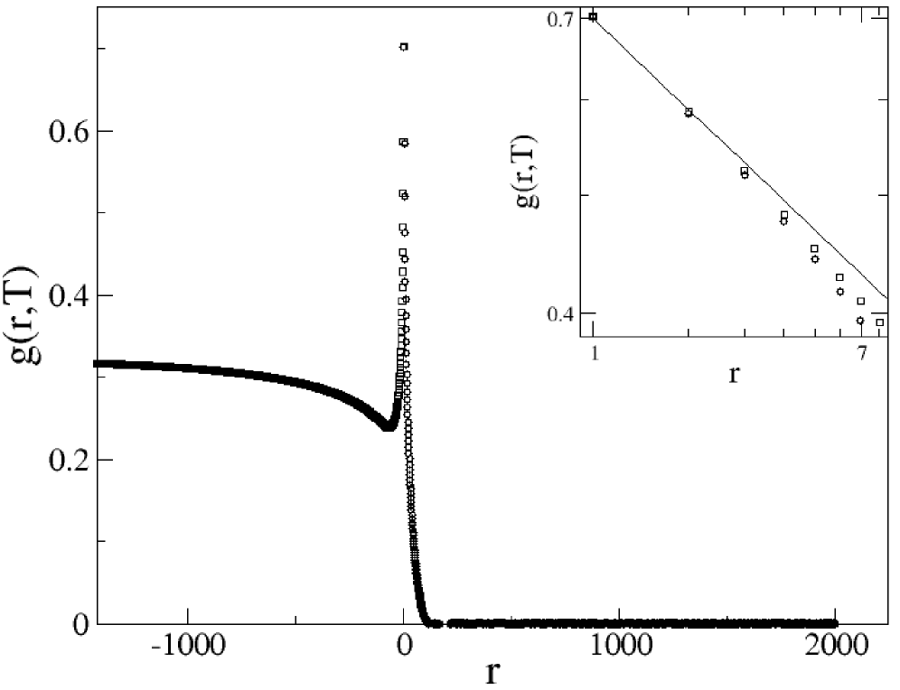
Figure 11: Plots of the correlation function $g(T,r)$, where the origin is taken just at the critical temperature. Here, for $r<0$ ($r>0$) one has $T<T_{c}$ ($T>T_{c}$). A rectangular lattice was used, with $L=5000$ and $M=100$. The temperature gradient was set between $T_{1}=0.8$ and $T_{2}=3.74$, respectively. Results obtained by averaging over $5\times 10^{5}$ Monte Carlo steps after disregarding the first $N_{D}=5\times 10^{5}$ Monte Carlo steps in order to allow for the stabilization of the system. The inset shows an enlarged view of the area close to criticality, on log-log scale. Squares (circles) correspond to correlations with spins in the direction of $T<T_{c}$ ($T>T_{c}$). The full line is a plot of the power law of $r$ with exponent $1/4=0.25$ and is shown for the sake of comparison. Absolute values of $r$ have been taken, in order to show both branches of $g(r)$. More details in the text.

Let us now discuss the results obtained in the present paper and perform comparisons to existing numerical results and/or exact values corresponding to the Ising magnet in a homogeneous thermal bath. Table I summarizes over seven independent estimations of the critical temperature as follows from the measurement of different physical observables in our gradient Ising system. In all cases we obtained an excellent agreement with the exact value, pointing out that the proposed gradient method is suitable for accurate determinations of critical points.

Type	Observable	$T_{c}$
Dynamic	Magnetization	2.2691(3)
Dynamic	Cumulant $U_{2}$	2.2691(3)
Dynamic	$2^{nd}$ order magnetization	2.2691(3)
Stationary	Cumulant $U_{2}$	2.284(1)
Stationary	Cumulant $U_{4}$	2.283(3)
Stationary	Scaling of $m$	2.282(3)
Stationary	Extrapolation of $T_{c}(L)$ from $\chi$	2.296(1)
Exactonsager	-	$\sim 2.26918$

Table 1: List of critical temperatures (third column) obtained by means of dynamic and stationary measurements, as listed in the first column. More details in the text.

Pointing now our attention to the measured critical exponents, we have already shown that our dynamic measurements of $d/z$, $\beta/\nu z$, and $\gamma/\nu z$ are fully consistent with a sort of ”dynamic” hyperscaling relationship (equation (21)). However, since the dimensionality entering in equation (21) appears in a quotient between exponents, more precisely as $d/z$ as follows from dynamic measurements of the cumulant, one needs independent measurements in order to obtain an unbiased estimation of $d$. The same reasoning applies to the dynamic exponent $z$. Therefore, we conclude that in order to obtain all the critical exponents we have to combine measurements corresponding to both the short-time dynamic simulations, namely, $d/z$, $\beta/\nu z$, and $\gamma/\nu z$, and stationary simulations, namely, $\beta/\nu$ and $d-2+\eta$. The results are shown in Table II, along with the values for the exponents that are known exactly ($\beta$, $\nu$, $\eta$, and $\gamma$), and the best available numerical results ($z$ and $\theta$), for the two-dimensional Ising model with a homogeneous thermal bath. It is worth mentioning that the error bars in each value were propagated from those of the original exponents, which in turn were calculated considering the values of the physical observables from the adjacent columns (at different temperatures) to the critical onefoot .

Exponent	Present work	Exact/numerical value
$\beta\;$	0.120(2)	1/8=0.125
$\nu\;$	0.96(7)	1
$\eta\;$	1.238(3)	5/4=1.25 (Details in the text)
$\gamma\;$	0.736(1)	3/4=0.75 (Details in the text)
$z\;$	2.16(4)	2.166(7)wang
$\theta\;$	0.196(6)	0.191(1)okano
$d\;$	1.02(8)	$-$

Table 2: List of the critical exponents (second column), along with the value of the dimensionality, obtained by combining dynamic and stationary measurements. The third column lists the exact value, in the first four rows, and the comparison value from numerical simulations, in the fifth and sixth rows.

There is an interesting result that involves both $\gamma$ and $\eta$ because the values obtained are different in a quantity of $1$ as compared with the exact values for the Ising ferromagnet for $d=2$, namely $\gamma=7/4$ and $\eta=1/4$. Furthermore, if we determine the values of $\gamma$ and $\eta$ from the scaling relationships $d\nu-2\beta=\gamma$ and $\gamma=\nu(2-\eta)$ by using the values of the exponents found in this work, we roughly reach the same results, namely $\gamma=0.74(8)$ and $\eta=1.23(8)$ respectively. The reason for this apparent disagreement becomes evident when we calculate, from the combination of dynamic and stationary results, the value of the effective dimensionality, obtaining $d=1.02(8)$, which strongly suggests $d=1$ as judged by the uncertainty interval. If we now use $d=1$ and re-calculate the exponents of the Ising ferromagnet, we obtain $\gamma=3/4=0.75$ and $\eta=5/4=1.25$, which are in perfect agreement with the exponents found by means of our simulations. This value for the effective dimensionality $d$ takes into account the fact that due to the presence of a thermal gradient, the thermodynamic functions are calculated as profiles of columns, thus lowering the effective dimensionality exactly by one unit.

5 CONCLUSIONS

We have studied, by means of Monte Carlo numerical simulations, the dynamic and stationary critical behavior of the two-dimensional Ising ferromagnet, in contact with a thermal bath that exhibits a linear gradient between low- and high- temperature extremes at $T_{1}$ and $T_{2}$ ($T_{2}>T_{1}$), respectively. It is worth mentioning that our proposed approach, is based on the assumption that the ferromagnet is in thermal equilibrium with the heat bath that intrinsically has a thermal gradient. This is in contrast to previous studies by other authors dgrad0 ; dgrad1 ; dgrad2 ; dgrad3 who placed only the extremes of the magnet in contact with two thermal baths at $T_{1}$ and $T_{2}$, and subsequently measured the thermal conduction between these baths. While for the numerical implementation of this ”conductivity approach” one needs to use a suitable ”Creutz demon” algorithmcreutz , our more straightforward approach can be implemented by means of standard algorithms, e.g., the Metropolis dynamics, just as in the present paper. Of course, our whole sample is out of equilibrium, but a key feature is that each column of the magnet (or sample in general) can be considered in equilibrium with the gradient thermal bath that is in contact with it. In this way, now one not only has information of the system under study for a wide range of temperatures ($T_{1}<T<T_{2}$), but also by means of a suitable choice of the temperatures of the extremes of the sample, such that $T_{1}<T_{c}<T_{2}$, where $T_{c}$ is the critical temperature, one can deal with samples simultaneously exhibiting the ordered and the disordered phases. In this way, instead of measuring average values of the physical observables at each $T$, one actually measures ”thermal profiles” of the observables averaged over ($d-1$)-dimensional columns of the sample. For this reason, the effective dimensionality entering in the scaling relationships is $d=1$.

Focusing our attention on the dynamic measurements, the measured thermal profiles allow us to simultaneously follow the time evolution of the sample for all temperatures of interest and, by drawing suitable plots, quickly identify the critical temperature (corresponding to a particular column) and determine the relevant critical exponents. Similarly, for the case of stationary measurements, we take advantage of the wide information available (critical temperature, critical exponents, correlation functions, etc.) that can be obtained just by performing a single simulation. The results obtained for the critical temperature and critical exponents are summarized and discussed in the context of Tables I and II, respectively. Based on that analysis, we conclude that the figures are remarkably accurate when one considers the computational effort involved. In fact, full agreement is obtained when our results are compared with exactly known values, e.g., for the critical temperature $T_{c}$, and the critical exponents $\beta$, $\nu$, $\gamma$, and $\eta$, as well as with the best available data taken from numerical simulations of other authors, e.g., for the exponents $\theta$ and $z$.

Based on the results presented and discussed in this paper, we conclude that the study of critical systems in the presence of a gradient of the suitable control parameter is a useful and powerful tool to gain rapid inshight on the behavior of the system, which could eventually be studied in further details by using more sophisticated methods . Furthermore, the studies of material systems under gradient conditions could shed light on the understanding of a wide variety of experimental and technologically useful situations.

ACKNOWLEDGMENTS. This work was financially supported by CICPBA, CONICET, UNLP and ANPCyT (Argentina).

References

- (1) K. Saito, S. Takesue, and S. Miyashita, Phys. Rev. E. 59, (1999) 2783.
- (2) M. Neek-Amal, R. Moussavi, and H. R. Sepangi, Physica A 371, (2006) 424.
- (3) M. Casartelli, N. Macellari, and A. Vezzani, Eur. Phys. J. B 56, (2007) 149.
- (4) E. Agliari, M. Casartelli, and A. Vezzani, Eur. Phys. J. B 60, (2007) 499.
- (5) E. Agliari, M. Casartelli and A. Vezzani, J. Stat. Mech., P07041 (2009).
- (6) E. Ising, Zeits. F. Physik 31, (1925) 253.
- (7) M. Tanaka, T. Wakamatsu, and H. Kobayashi, IEEE Trans. J. Magn. Japan 2, (1987) 728.
- (8) M. M. Schwickert, K. A. Hannibal, M. F. Toney, M. Best, L. Folks, J.-U. Thiele, A. J. Kellock, and D. Weller, J. Appl. Phys. 87, (2000) 6956.
- (9) L. YoongXiong, E. Ahmad, Y. Xu and K. Barmak, IEEE Trans. Magn. 41, (2005) 3328.
- (10) M. Creutz, M, Phys. Rev. Lett. 50, (1983) 1411.
- (11) L. Kadanoff and J. Swift, Phys. Rev. 165, (1968) 310.
- (12) G. Y. Vichniac, Physica D, 10, (1984) 96.
- (13) Kittel, C., Introduction to Solid State Physics, Eighth ed., John Wiley & Sons, Inc; USA (2005)
- (14) E. V. Albano, M. A. Bab, G. Baglietto, R. A. Borzi, T. S. Grigera, E. S. Loscar, D. E. Rodriguez, M. L. Rubio Puzzo, and G. P. Saracco, Rep. Prog. Phys. 74, (2011) 026501.
- (15) L. Onsager, Phys. Rev. 65, (1944) 117.
- (16) It is worth mentioning that by setting the dependence of the observables on the horizontal coordinate along the thermal gradient is supresed.
- (17) H. K. Janssen, B. Schaub, and B. Schmittmann, Z. Phys. B 73 (1989) 539.
- (18) K. Binder, Rep. Prog. Phys. 60, (1997) 487.
- (19) K. Christensen, and N. R. Moloney, Complexity and Criticality, (Imperial College Press, London, 2005).
- (20) It is worth mentioning that the error bars only account for the changes in the values of the physical observables when adjacent columns are considered, and an error of the order of is introduced in the temperature. So, our reported error bars have to be enlarged when considering both statistical errors and scaling corrections that are ignored.
- (21) K. Okano, L. Schülke, K. Yamagishi, and B. Zheng, Nucl. Phys. B 485, (1997) 727
- (22) F. G. Wang, and C. K. Hu, Phys. Rev. E 56, (1997) 2310